


 nueva página del texto (beta)
 Inglés (pdf)
 Artículo en XML
 Referencias del artículo
 Enviar artículo por email
 Citado por SciELO
  Similares en
SciELO
Similares en
SciELO 
 Permalink
1. INTRODUCTION
The management of the adverse impacts of global warming is one of the fundamental challenges facing capitalism over the coming decades. The anthropogenic greenhouse gas (GHG) emission, the major source of global warming, is estimated to have caused approximately 1.0ºC of global warming above pre-industrial levels (Intergovernmental Panel on Climate Change, IPCC, 2018).
The Paris Agreement, which 182 countries and the European Union (EU) have ratified, aims to hold the increase in “the global average temperature well below 2ºC above pre-industrial levels and pursues efforts to limit the temperature increase to 1.5ºC above pre-industrial levels” (United Nations Framework Convention on Climate Change, UNFCCC, 2015, p. 2). Climate scenarios suggest that for limiting temperature below 2.0ºC increase, carbon dioxide, CO2 emissions, the main pollutant, must decline by about 20% from 2010 levels by 2030. For the limited overshoot of 1.5ºC increase, CO2 emissions must decline by about 45% by 2030 (IPCC, 2018).
This context has, at least, two economic aspects. First, consistent policy proposals for reducing global CO2 emissions need to take a macroeconomic perspective that measures the current cost in terms of Gross Domestic Product (GDP). Second, although all countries of the earth will experience the impact of global warming, the countries may have very different costs and benefits from mitigation and adaptation policies (Foley, 2003). The ecological macroeconomics is moving towards the construction of a theoretical framework and empirical models that examine these issues from an alternative perspective (Rezai, Taylor, and Mechler, 2012; Kemp-Benedict, 2018; Taylor, Rezai, and Foley, 2016).
This paper intends to contribute in this regard. First, we design an empirical strategy derived from an ecological-economic framework in which the gdp and CO2 emissions are produced employing capital, energy and labor (Brock and Taylor, 2010; Kurz, 2006; Baumgärtner et al., 2001). A nonparametric method, the local polynomial regression, is employed to investigate regularities on technical change and the production of gdp and CO2 emissions for 84 countries between 1980 and 2014. The country sample is selected from a new data set, the Extended Penn World Tables v.6.0 (EPWT v.6.0). This new data may shed some fresh light on discussions of the climate policy literature regarding the principle of differentiated responsibilities and respective capabilities.
Our second contribution is the derivation of an expanded version of the Kaya identity to explore links between the growth rate of CO2 emissions, capital accumulation and the parameters of technical change, especially movements towards environment-saving techniques (Rezai, Taylor, and Mechler, 2012). This modified Kaya identity is employed to discuss normative issues related to the intended nationally determined contributions (INDCs). The INDC is the greenhouse gas target assumed by each country, representing the national efforts to reduce emissions and adapt to the impacts of global warming. Employing the current trend, we compute the required pace of capital accumulation, energy efficiency and emission intensity to accomplish the emission targets reported on the INDCs. This analysis offers a first look at the distribution of the economic efforts of the Paris Agreement.
The results are presented in line with Kaldor (1961) who in the mid-20th century stated that economic theory has to explain the regularities or stylized facts of economic growth. We find evidence of a global relative decoupling from the second half of the 1970s. The developed countries have a low CO2 emissions growth rate, with some of them presenting evidence of absolute decoupling, while the developing countries with high GDP growth have a high growth rate of CO2 emissions. The countries with absolute decoupling presented a movement towards environment-saving technical change, with remarkable improvements on the energy-labor ratio and the capital-energy ratio.
The modified Kaya identity suggests that the individual voluntary definition of the emission targets under the Paris Agreement has resulted in an unequal distribution of the future abatement efforts among developing and developed countries. In the absence of energy or environment-saving technical change, sharper reductions in the pace of accumulation in developing countries are required to comply with the individual emission targets.
The paper is organized as follows. Section two presents the ecological-economic framework. Section three presents the methods and data. Section four analyzes the production of both outputs, the techniques of production, and the emission intensity variables for 84 countries between 1980-2014. The patterns of technical change, the evidence of the decoupling between CO2 emissions and economic growth and the Paris Agreement targets are explored in subsection 4.1 and 4.2. Finally, section five concludes the paper.
2. THE LINK BETWEEN CO2 EMISSIONS AND ECONOMIC ACTIVITY
This study uses an ecological-economic framework as a theoretical baseline motivation for the empirical strategy. The framework is inspired by contributions in both environmental and ecological macroeconomics that considers the environment as a sink for production waste. This literature investigates the links between economic growth and the environment (Brock and Taylor, 2010; Kurz, 2006; Baumgärtner et al., 2001). More importantly, this framework allows us to employ the Kaya decomposition to investigate the links between economic growth and technical change in GDP and CO2 emissions.
The economy produces GDP, which we denote by X, and the carbon dioxide, B, by using physical capital, K, energy, E, and labor, N. The GDP includes the depreciation, D, of physical capital and excludes intermediate inputs from production. However, the production of intermediate inputs also generates CO2 emissions. Physical capital depreciates every year at the rate d, the total depreciation included in GDP is equal to dK. The main source of pollution results from the employment of energy generated by oil, coal and other chemicals to produce GDP.
The production process involves the combination of physical capital, energy and labor to produce two outputs and depreciated capital. The central role of energy in the production process is considered. This is an idea widely accepted among ecological economists, but never fully considered by the professional mainstream. The process represented in upper part of Table 1 includes three inputs and two outputs.
Table 1 The input-output production process
| Input | Output | ||||
|---|---|---|---|---|---|
| Level | |||||
| Capital | Energy | Labor | gdp | CO2 | Capital |
| K | E | N | X | B | K - D |
| Intensive units | |||||
| Capital | Energy | Labor | gdp | CO2 | Capital |
| k | e | 1 | x | b | (1 - d)k |
A production technique is defined in terms of a labor unit. We divide the levels of inputs and outputs by labor, N, obtaining the capital-labor ratio, k, the energy-labor ratio, e, the GDP-labor ratio or labor productivity, x, the CO2 emissions per labor ratio, b. A technique is defined by the parameters k, e, x, b, and d. Table 1 displays in its lower part the production process in terms of labor input as an input-output matrix for a production technique. The technology is the set of all known techniques.
Additionally, we define other variables in terms of capital, energy and GDP. We consider the productivity of each input for both outputs. The productivity of capital is equal to the GDP-capital ratio, p = X/K, the productivity of energy is equal to the GDP-energy ratio, s = X/E. For CO2 we define the emissions per unit of capital, a = B/K, and the emissions per unit of energy, m = B/E. Two additional useful relationships are the ratios between capital and energy, u = K/E, and between the CO2 and GDP, o = B/X.
The process of capital accumulation, the conversion of profits into capital through investment, expands both outputs. The GDP is either consumed or invested, improving life conditions. The CO2 emissions are dispersed and accumulated in the atmosphere to the point that it is currently generating global warming. The accumulation of capital involves a technical change which modifies the technical parameters k, e, x, b, and p, as well as s, a, m, u, and o.
We denote the growth rate of the variable x as g x , that is, the difference between the labor productivity in the year of study and its value in the previous year divided by its value in the previous year. The literature distinguishes four types of technical change based on the growth rates of labor productivity and capital productivity. Purely labor-saving or Harrod-neutral technical change corresponds to a rise in labor productivity, g x > 0, and a constant capital productivity, g p = 0. Purely capital-saving or Solow-neutral technical change corresponds to a rise in capital productivity, g p > 0, and a constant labor productivity, g x = 0. Equally input-saving or Hicks-neutral technical change corresponds to an identical change in labor and capital productivities, g x = g p . The combination of a labor-saving, g x > 0, and capital-using, g p < 0, technical change was labeled by Foley and Michl (1999) as Marx-biased technical change.
From an ecological perspective, it is natural to expand the taxonomy of technical change to include energy. The energy-saving technical change is a rise in energy productivity, g s > 0. Purely energy-saving technical change corresponds to a rise in energy productivity with constant labor and capital productivities, g x = 0, g p = 0. Now, a purely labor-saving technical change corresponds to a rise in labor productivity, g x > 0, a constant capital productivity, g p = 0, and a constant energy productivity, g s = 0. A purely capital-saving technical change corresponds to a rise in capital productivity, g p > 0, a constant labor productivity, g x = 0, and a constant energy productivity, g s = 0. Equally input-saving technical change corresponds to an identical change in labor, capital and energy productivities, g x = g s = g p > 0.
In addition, the Marx-biased technical change can be related to an energy-saving or energy-using pattern. The Marx-biased technical change is also energy-saving when the growth rate of energy productivity increases, g s > 0. Otherwise, the Marx-biased technical change is energy-using.
We also define technical change from an environment perspective. Labor environment saving technical change corresponds to a decline of CO2 emission per labor input, g b < 0. Capital environment saving technical change corresponds to a fall in CO2 emission per capital, g a < 0. Energy environment saving technical change corresponds to a decline in CO2 per energy, g m < 0. Hence, the patterns of technical change can be “clean” or “dirty” according to its impact on CO2 emissions.
It is possible to establish several relationships between the technical change in gdp and CO2 emissions. For instance, we have o = (B/X) = (B/N)(N/X) = (B/K)(K/X) = (B/E)(E/X) = b/x = a/p = m/s and g o = g b - g x = g a - g p = g m - g s . From this perspective, we can also derive an expanded version of the Kaya identity. The Kaya identity determines the impact of anthropogenic activity on the ecosystem and has a central role in the forecasting of future scenarios for climate change on the ipcc reports. Substituting the population by the number of workers, the Kaya identity is equal to:
Using the previous definition of the variables, and computing its rate of growth, we have:
In turn, g s can be decomposed in g s (( g p + g u . Thus, we can expand the Kaya identity to consider the role of technical change. Hence:
The growth rate of CO2 emissions is decomposed as the sum between the growth rates of labor inputs, labor productivity, and CO2 emissions per energy minus the growth rates of capital productivity and capital-energy ratio. The expanded Kaya identity provides a link between the expansion of CO2 emissions and the parameters of technical change that we will explore using empirical data.
Our results below suggest that the elasticity of CO2 emissions with respect to labor is zero. In this case, we can rewrite the Kaya identity in terms of the capital stock and energy in the following way:
Hence, the proportional rate of growth can be written as:
Now, the growth rate of CO2 emissions is positively associated to capital accumulation, g K , and the growth rate of CO2 emissions by unity of energy, g m , and negatively associated to the growth rate of the ratio of capital to energy, g u . Using [5], we compute the required pace of capital accumulation, energy efficiency and emission intensity to accomplish the emissions targets reported on the indcs. The analysis is based on the growth rates computed between 1980 and 2014.
3. METHODS AND DATA
This study is organized in two main parts. First, the investigation on the regularities between CO2 emission and economic activity. Second, a simple simulation of the required pace of capital accumulation, energy efficiency, and emission intensity to comply with the emissions targets reported in the INDCs of the Paris Agreement.
The empirical regularities of 84 countries between 1980-2014 are explored through the utilization of local regression, a non-parametric method that employs smoothing to fit curves and surfaces. It estimates a smooth curve between variables without assuming a previous functional form (Cleveland, 1993), allowing us to visualize the relationship between the variables. The basic ideas of the method can be expressed considering the model:
where y i is the dependent variable and x pi are the p independent variables, and ( i are the errors that are assumed to be normally and independently distributed with zero mean and constant variance. The goal is to estimate the regression function f without references to a previous functional form. This estimation is obtained defining a neighborhood in the space of independent variables which comprises a subset of observations that are closest to x. The neighborhood size is defined by the bandwidth, (, 0 < ( ( 1, that indicates the proportion of points of the total observations that are considered in the computation of the smoothed function. It controls the smoothness of the fit. Generalized Cross Validation and Akaike’s Information Criterion were used in the bandwidth definition.
The bandwidth defines a neighborhood in the space of independent variables, the points in this space are weighted according to their distance to x. The points closest to x have large weight, the points far from x have lower weight. The weight function employed in the estimates in this paper was the gaussian function. Moreover, it is necessary to choose the degree of the polynomial of the independent variables that are fitted to the dependent variable. The degree of fit was chosen by a series of local regression plots according to the recommendations by Loader (1999). This procedure defines the value of the estimated function at the point x. It is repeated for each point of interest to obtain the estimated function.
Loader (1999) and Cleveland and Devlin (1998) suggest a series of graphs to check the assumptions of normality and constant variance of the residuals. The statistical properties of local regression have been studied, allowing to calculate confidence intervals and to realize tests of hypothesis. Cleveland and Devlin (1988) and Fan and Gijbels (1996) present the basic conception of the statistical inference in local regression. The confidence intervals in the paper are computed locally, pointwise confidence interval. Loader (1999) discusses the difference between pointwise and simultaneous confidence intervals.
In order to evaluate the required economic and technical changes to comply with the Paris Agreement (UNFCCC, 2015), we proceed to analyze the INDCs submitted by each of the twenty major global CO2 emitters. These countries answer for 77.20% of total emissions in the sample. The great flexibility of the Paris Agreement has led to a lack of homogeneity on the definition of the emission targets. Some countries have defined targets over the level of emissions, while others over the emissions intensity. In addition, the lack of homogeneity extends also to the definition of individual pollutants that will be targeted.
We first homogenize data and categorize the information by computing the target in terms of the level of CO2 emissions. The CO2 emissions are the major source of GHG emissions (IPCC, 2018). The EU is one of the Parties at the UNFCCC. The EU and its member have committed to a target of at least 40% domestic reduction in GHG emissions by 2030 compared to 1990, to be jointly fulfilled. As the country-specific responsibilities are unclear, we defined a uniform emission target of 40% applied to all the EU members.
The data set is the EPWT v.6.02. It is organized using the Penn World Table (Feenstra, Inklaar, and Timmer, 2015) and other resources. The source for CO2 emissions is Boden, Marland, and Andres (2015) that measures the emissions from fossil fuel consumption and cement production. For energy, the data source is World Bank (2017). The EPWT presents homogeneous data for a large number of countries for the years between 1967 and 2014. However, the methodological procedure to compute some of the EPWT variables is subject to criticisms discussed in the respective documentation.
The monetary variables, the GDP, the standardized fixed capital stock and the estimated depreciation are expressed in purchasing power parity, 2011 international dollars. The standardized fixed capital stock and depreciation is computed using the perpetual inventory method. The labor input is the number of employed people. The energy is computed in kilograms of oil equivalent. The CO2 emissions is measured in kilograms of carbon.
4. EVOLUTION OF THE PRODUCTION OF GDP AND CO2 EMISSIONS
Figure 1 presents the world growth rates of CO2 emissions, the broken lines, and the GDP, the continuous lines, in the 1951-2014 period. The thick line shows the nine years mean growth rates and the thin line the annual growth rates. The GDP data disregard the countries that were members of the former Soviet Union. There is a positive correlation for the annual growth rates. However, the growth rates of CO2 emissions were larger than the GDP growth rates between 1950s and the early 1970s. This period corresponds to the reconstruction of Europe and the industrial expansion of the United States and the former Soviet Union during the Cold War.
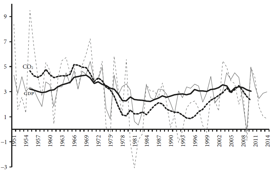
Source: Conference Board (2017) and Boden, Marland, and Andres (2015).
Figure 1 World growth rates of GDP and CO2 emission, 1951-2014 (percentages)
In the second half of the 1970s, the GDP began to grow at a higher rate than the CO2 emissions. Between 1980 and 2014, CO2 emissions grew by 1.8% per year, while the GDP expanded at 2.6% annually. Hence, there is evidence of relative decoupling between CO2 emissions and economic growth. A relative decoupling occurs when the growth rate of the environmentally relevant variable is less than the GDP growth for a given period (Organisation for Economic Co-operation and Development, OECD, 2002). We will investigate this evidence starting with cross-country considerations before turning to the evolution of GDP production and CO2 emissions.
Table 2 compiles the ranking and the share in CO2 emissions and the GDP ranking of the main CO2 emitters in 1980 and 2014. It also presents the growth rates of both outputs between these years. There are 163 countries in the sample. China was the country with the largest CO2 emissions in 2014, generating 28.5% of the total, with United States (US) taking the second position. India expanded very rapidly its emissions, moving to the third place. These three countries answered for almost half of the CO2 emissions in 2014, well above the one third observed in 1980.
Table 2 Ranking, share, and growth rate of CO2 emissions and gdp growth rate by main emitters, 1980 and 2014
| Country | Ranking in B | Share in B (%) | Ranking in X | Ranking in B | Share in B (%) | Ranking in X | Increase in B (%) | Increase in X (%) |
|---|---|---|---|---|---|---|---|---|
| 1980 | 2014 | |||||||
| China | 2 | 7.5 | 3 | 1 | 28.5 | 1 | 601.5 | 1 010.7 |
| United States | 1 | 24.3 | 1 | 2 | 14.5 | 2 | 11.2 | 146.8 |
| India | 8 | 1.6 | 9 | 3 | 6.2 | 3 | 612.8 | 766.1 |
| Russia | n.a. | n.a. | n.a. | 4 | 4.7 | 6 | n.a. | n.a. |
| Japan | 3 | 4.9 | 2 | 5 | 3.4 | 4 | 28.1 | 103.2 |
| Germany | n.a. | n.a. | 4 | 6 | 2.0 | 5 | n.a. | n.a. |
| Iran | 18 | 0.6 | 34 | 7 | 1.8 | 18 | 437.2 | 925.3 |
| Saudi Arabia | n.a. | n.a. | n.a. | 8 | 1.7 | 17 | n.a. | n.a. |
| South Korea | 17 | 0.7 | 22 | 9 | 1.6 | 13 | 335.4 | 823.4 |
| Canada | 6 | 2.3 | 11 | 10 | 1.5 | 14 | 21.2 | 154.8 |
| Brazil | 14 | 1.0 | 10 | 11 | 1.5 | 7 | 183.2 | 376.1 |
| South Africa | 10 | 1.2 | 18 | 12 | 1.4 | 29 | 114.4 | 147.9 |
| Mexico | 9 | 1.4 | 8 | 13 | 1.3 | 12 | 78.9 | 134.8 |
| Indonesia | 20 | 0.5 | 14 | 14 | 1.3 | 10 | 389.7 | 648.6 |
| United Kingdom | 4 | 3.0 | 6 | 15 | 1.2 | 9 | -27.5 | 121.3 |
| Australia | 11 | 1.1 | 16 | 16 | 1.0 | 19 | 63.7 | 222.8 |
| Turkey | 23 | 0.4 | 15 | 17 | 1.0 | 15 | 356.7 | 360.8 |
| Italy | 7 | 2.0 | 7 | 18 | 0.9 | 11 | -17.6 | 88.3 |
| Thailand | 34 | 0.2 | 28 | 19 | 0.9 | 24 | 687.9 | 482.3 |
| France | 5 | 2.6 | 5 | 20 | 0.8 | 8 | -40.0 | 104.5 |
| Other countries | 44.7 | 23.0 | ||||||
Note: n.a. - information is not available.
Source: EPWT v.6.0.
CO2 emissions increased for most of the bigger emitters between 1980 and 2014, except for United Kingdom, Italy and France. It indicates the presence of absolute decoupling in these countries, as detailed below. These three countries displayed the lowest GDP growth rate in the period, around 100%. Another group of developed countries, US, Canada and Japan, increased their emissions in less than 30%, while the GDP expanded around 150% in the first two and 100% in Japan.
The developing countries in Asia, with the leadership of Thailand, India and China, multiplied their emissions by a factor between four and seven during the period. The Asian countries also led the expansion in GDP, with impressive growth rates. In Latin America and in Africa, the developing countries raised their emission by a factor between 0.7 and two with GDP growth rates somewhat above the developed countries. There was a link between the GDP growth rate and the rise in CO2 emissions. The developing countries moved up in the rankings of GDP production and CO2 emissions.
The direct relationship between GDP and CO2 emissions observed in Table 2 is a regular pattern for many countries worldwide. In Figure 2 there appears the estimated local regression fits between the logarithms of GDP and CO2 emissions for 84 countries in 1980 and in 2014. Generally, a country with a higher GDP shows higher CO2 emissions than a country with a smaller GDP.
There are two important aspects in Figure 2. First, the emissions per unit of GDP diminished between 1980 and 2014, the line for 2014 is below the line for 1980. The elasticity of CO2 emissions with respect to GDP declined from 1.137 in 1980 to 1.031 in 20143. Interestingly, however, the elasticity remains relatively unchanged for the countries with the lowest GDPs. Second, the total emissions grew in absolute terms as the observed points for most countries and the fitted line moved over time in the northeast direction.

Source: EPWT v.6.0.
Figure 2 GDP and CO2 emissions and the local regression fits for 84 countries, 1980 and 2014 (local regression parameters: bandwidth = 0.48 for 1980 and 0.46 for 2014, degree = 3)
Figure 3 shows the local regression fits between the logarithms of GDP, the left-hand column, and CO2 emissions, the right-hand column, and the logarithms of labor, capital and energy for 84 countries in 1980 and 2014. The higher use of inputs appears as a movement to the right of the 2014 points in relation to the 1980 ones. All estimated local regression fits display a positive association between inputs and outputs.
There is a greater dispersion between labor inputs and GDP and CO2 emissions than in the case of capital and energy. The production of the same amount of GDP in 2014 required lower quantities of labor and energy and a similar quantity of capital than in 1980. The estimated local regression fit between labor and energy and GDP for 2014 is above the fit for 1980, while the relationship between capital and GDP displayed minor changes between 1980 and 2014. The CO2 emissions in 2014 with respect to labor inputs and energy displayed minor changes in comparison to 1980. There was a clear reduction in emissions with respect to capital. Therefore, the average capital stock is getting relatively cleaner, which reveals a possible movement towards the adoption of capital environment saving technical change.

Source: EPWT v.6.0.
Figure 3 Relationship between inputs and GDP and CO2 emissions and the local regression fits, 1980 and 2014 .(local regression parameters: top left graph: bandwidth = 0.37 for 1980 and 0.35 for 2014, degree =1; top right graph: bandwidth = 0.33 for 1980 and 0.35 for 2014, degree =1; middle left graph: bandwidth = 0.37 for 1980 and 0.34 for 2014, degree = 1; middle right graph: bandwidth 0.33 for 1980 and 0.33 for 2014, degree = 1; lower left graph: bandwidth = 0.47 for 1980 and 0.48 for 2014 and degree =1; lower right graph: bandwidth = 0.37 for 1980 and 0.35 for 2014, and degree =1)
We estimated elasticities of GDP and CO2 emissions with relation to labor, capital and energy. All the input elasticities of GDP are positive and significant at the 1% level4. The capital elasticity of GDP is the largest and increased between 1980 and 2014, from 0.567 to 0.667. The energy elasticity of GDP is around 0.195, almost the same value for the two years. The labor elasticity of GDP decreased from 0.204 to 0.148. The CO2 emissions elasticities with respect to capital and energy are significant at 1% in both years. The capital elasticity of CO2 emissions increased from 0.415 to 0.546 between 1980 and 2014, while the energy elasticity of CO2 emissions diminished from 0.971 to 0.563. The labor elasticity of CO2 emissions was negative, significant at 1% in 1980, and not statistically different from zero at five percent of significance in 2014.
Changes in the employment of labor, while capital and energy are held constant, do not affect the CO2 emissions. Schor (2010) suggests that lower working hours may reduce unemployment and CO2 emissions. Lower working hours would require the employment of labor, which is a clean input.
Figure 4 presents the relationship between the productivities of each input and the corresponding emission intensities for 1980 and 2014. One can observe an improvement in the relationship between productivity and emissions per input in the period. There is a positive association between labor productivity and the emissions per worker, but its elasticity is remarkably smaller in 2014. It may be related to the improvements in the CO2 emissions per unit of capital. The countries with high-energy productivity are also those with relatively high CO2 emissions per unit of energy. The capital productivity and the emissions-capital ratio are positively correlated. There is a fall in CO2 emissions per input after certain threshold consistent with an environment Kuznets curve.

Source: EPWT v.6.0.
Figure 4 Relationship between input productivity and input emission intensity, 1980 and 2014. (local regression parameters: upper graph: bandwidth = 0.42 for 1980 and 0.55 for 2014, degree = 3; middle graph: bandwidth = 0.47 for 1980 and 0.47 for 2014, degree = 3; lower graph: 0.46 for 1980 and 0.44 for 2014, degree = 1)
In Figure 5, the upper graphs relate capital-labor ratio with labor productivity and CO2 emissions per worker for 1980 and 2014. In the lower graphs, the energy-labor ratio replaces the capital-labor ratio. The local regression fits for 1980 and 2014 display two results. First, there is a concave shape in the relationship between labor productivity and capital-labor ratio and between CO2 emissions per worker and the capital-labor ratio. Similar results occur in the relationship between labor productivity and energy-labor ratio and between CO2 emissions per worker and energy-labor ratio. Again, these results are congruent with an environment Kuznets curve. Second, a given level of capital-labor and energy-labor ratios produced higher labor productivity and lower amount of CO2 per worker in 2014 in relation to 1980, which is compatible with relative decoupling.

Source: EPWT v.6.0.
Figure 5 Relationship between capital-labor and energy-labor ratios and labor productivity and CO2 emissions per worker, 1980 and 2014. (local regression parameters: top left graph: bandwidth = 0.47 for 1980 and 0.47 for 2014, degree =1; top right graph: bandwidth = 0.34 for 1980 and 0.36 for 2014, degree =1; lower left graph: bandwidth = 0.37 for 1980 and 0.34 for 2014, degree = 1; lower right graph: bandwidth 0.39 for 1980 and 0.42 for 2014, degree = 1)
Figure 6 relates labor productivity with capital and energy productivities on the left column and the CO2 emissions per worker with CO2 emissions per capital and energy on the right column for 1980 and 2014. There is a negative correlation between capital productivity and labor productivity, and a positive association between energy productivity and labor productivity.

Source: EPWT v.6.0.
Figure 6 Relationship between input productivities and CO2 emissions per input, 1980 and 2014. (local regression parameters: bandwidths = 0.53 and 0.55; 0.55 and 0.57; 0.53 and 0.55; 0.56 and 0.57, degree = 1)
In the case of CO2 emissions per unit of inputs, there is a direct relationship between emissions per capital and emissions per worker and a concave relationship between emissions per capital and the emissions per energy. Thus, in the growth process there is an increase in labor and energy productivities and a decline in capital productivity that is consistent with a Marx-biased pattern of technical change.
4.1. Patterns of technical change and the evidence of absolute decoupling
In recent years, an important research field that analyses the evidence of absolute decoupling of CO2 emissions from economic growth has emerged. According to OECD (2002, p. 11), absolute decoupling occurs “when the growth rate of the environmentally damaging variable is zero or negative” despite GDP growth. The evidence of decoupling is surrounded by controversies that are at the center of the debate on the growth limits.
The evidence of absolute decoupling is heterogeneous (Naqvi and Zwickl, 2017); while some studies focus on aggregate CO2 and GDP, others investigate the multisectoral emissions. From our production framework and the decomposition of the expanded Kaya identity we explore the evidence of absolute decoupling looking at the patterns of technical change.
Table 3 shows the information on technical change for the biggest CO2 emitters for the years without and with absolute decoupling between 1980 and 2014, highlighting the parameters of the expanded Kaya identity. After investigating the data by visual inspection, we computed the correlation between the time series. The years with absolute decoupling displayed a negative correlation between the logarithms of GDP and CO2 emissions.
Table 3 Technical change and the expanded Kaya identity for the main CO2 emitters in periods without and with absolute decoupling, annual compound growth rate (percentage), 1980-2014
| Country | No absolute decoupling | g s | g a | g b | g o | g e | Expanded Kaya identity | |||||
|---|---|---|---|---|---|---|---|---|---|---|---|---|
| g x | g p | g u | g m | Technical effect | g N | |||||||
| China | 1980-2014 | 2.27 | -3.93 | 4.23 | -1.35 | 3.31 | 5.58 | -2.57 | 4.84 | 0.91 | 4.22 | 1.5 |
| United States | 1980-2005 | 2.15 | -2.28 | -0.52 | -2.31 | -0.36 | 1.79 | 0.03 | 2.12 | -0.16 | -0.52 | 1.34 |
| India | 1980-2014 | 2.18 | -0.52 | 3.26 | -0.57 | 1.65 | 3.83 | 0.05 | 2.13 | 1.61 | 3.26 | 2.52 |
| Russia | 2007-2014 | 3.48 | -0.26 | 0.13 | -3.86 | 0.52 | 4 | 3.61 | -0.13 | -0.39 | 0.13 | 0.19 |
| Japan | 1980-2014 | 1.34 | -1.17 | 0.42 | -1.36 | 0.44 | 1.78 | 0.19 | 1.15 | -0.02 | 0.42 | 0.31 |
| Iran | 1980-2014 | 1.47 | 0.76 | 2.05 | -1.9 | 2.48 | 3.95 | 2.66 | -1.19 | -0.44 | 2.04 | 2.9 |
| Saudi Arabia | 1987-2014 | 1.63 | 1.75 | 0.22 | -2.41 | 1 | 2.63 | 4.17 | -2.54 | -0.78 | 0.22 | 4.03 |
| South Korea | 1980-2014 | 1 | -2.91 | 2.37 | -2.21 | 3.58 | 4.58 | -0.7 | 1.7 | -1.21 | 2.37 | 1.96 |
| Canada | 1980-2008 | 1.86 | -2.25 | -0.78 | -2.29 | -0.35 | 1.51 | 0.04 | 1.82 | -0.43 | -0.78 | 1.63 |
| Brazil | 1980-2014 | 1.71 | -1.59 | 0.84 | -1.53 | 0.66 | 2.37 | -0.06 | 1.77 | 0.18 | 0.84 | 2.22 |
| South Africa | 1980-2009 | -0.13 | 1.12 | 0.52 | 0.08 | 0.56 | 0.43 | 1.04 | -1.17 | -0.05 | 0.51 | 2.21 |
| Mexico | 1980-2014 | 0.51 | -1.24 | -0.98 | -0.8 | -0.69 | -0.18 | -0.44 | 0.95 | -0.29 | -0.98 | 2.69 |
| Indonesia | 1980-2014 | 1.82 | -3.4a/ | 2.38 | -1.25 | 1.8 | 3.62 | -2.34 | 4.16 | 0.57 | 2.37 | 2.3 |
| United Kingdom | 1980-1989 | 1.58 | -1.76 | -0.66 | -1.99 | -0.24 | 1.34 | 0.24 | 1.34 | -0.42 | -0.66 | 0.7 |
| Australia | 1980-2009 | 1.51 | -1.36 | 0 | -1.6 | 0.08 | 1.59 | 0.24 | 1.27 | -0.08 | 0 | 2.01 |
| Turkey | 1980-2014 | 0.52 | 1.48 | 2.8 | -0.02 | 2.31 | 2.83 | 1.51 | -0.99 | 0.49 | 2.8 | 1.66 |
| Italy | 1980-2004 | 0.61 | -2.29 | 0.31 | -1.24 | 0.94 | 1.55 | -1.05 | 1.66 | -0.63 | 0.31 | 0.51 |
| Thailand | 1980-2014 | -0.15 | 0.14 | 4.49 | 0.89 | 3.75 | 3.6 | -0.75 | 0.6 | 0.74 | 4.49 | 1.58 |
| Country | Absolute decoupling | g s | g a | g b | g o | g e | g x | g p | g u | g m | Technical effect | g N |
| United States | 2005-2014 | 1.87 | -2.23 | -1.42 | -2.44 | -0.85 | 1.02 | 0.21 | 1.66 | -0.57 | -1.42 | 0.34 |
| Germany | 1991-2014 | 3.05 | -2.6 | -1.53 | -3.66 | -0.92 | 2.13 | 1.06 | 1.99 | -0.61 | -1.53 | 0.42 |
| Canada | 2008-2014 | 0.56 | -3.7 | -1.79 | -1.69 | -0.66 | -0.1 | -2.01 | 2.57 | -1.13 | -1.79 | 1.07 |
| South Africa | 2009-2014 | 2.79 | -6.04 | -3.85 | -3.39 | -3.26 | -0.47 | -2.65 | 5.44 | -0.6 | -3.86 | 3.32 |
| United Kingdom | 1989-2014 | 3.02 | -3.84 | -1.91 | -3.75 | -1.19 | 1.83 | -0.1 | 3.12 | -0.72 | -1.91 | 0.61 |
| Australia | 2009-2014 | 2.8 | -4.68 | -3.73 | -4.33 | -2.21 | 0.59 | -0.35 | 3.15 | -1.53 | -3.74 | 1.96 |
| Italy | 2004-2014 | 3.86 | -5.38 | -3.66 | -5.3 | -2.22 | 1.64 | -0.08 | 3.94 | -1.44 | -3.66 | -0.26 |
| France | 1980-2014 | 1.42 | -3.4 | -2.03 | -3.61 | 0.15 | 1.57 | 0.2 | 1.22 | -2.19 | -2.04 | 0.53 |
Note: a/ - period 1982-2014.
Source: EPWT v.6.0.
There is no evidence of absolute decoupling between CO2 emissions and economic growth for 12 countries for the period. Most of them were developing countries. China, Brazil, Indonesia and South Korea followed a Marx-biased and an energy saving technical change. Thailand displayed a Marx-biased and energy using technical change and raising CO2 emissions per GDP. India, Russia, Japan, Turkey, Iran and Saudi Arabia exhibited an input-saving technical change in capital, labor and energy; Mexico showed declining labor and capital productivities and raising energy productivity. These countries, except Mexico, displayed a labor environment using technical change.
Table 3 reveals a positive association between the growth rates of labor productivity, energy-labor ratio and CO2 emissions per worker. The ratio between CO2 emissions and energy rose in developing countries with a Marx-biased technical change, plus India and Turkey. The other countries experienced an energy environment saving technical change. Most countries also experienced a capital environment saving technical change except for Iran, Saudi Arabia, Thailand and Turkey.
Five developed countries and South Africa shifted from no absolute decoupling to absolute decoupling during the period of study. It occurred around the financial crisis, excluding United Kingdom. We first investigate the years without absolute decoupling. Italy displayed a Marx-biased, energy saving technical change. United States, Canada, Australia and United Kingdom followed an input saving technical change. South Africa showed a labor and capital saving and an energy using technical change.
In the United States, Canada, and United Kingdom occurred an environment saving technical change in the three inputs. Interesting, labor productivity rose in these countries without a correspondent increase in the energy-labor ratio, which is explained by the relatively high growth rate of energy productivity. From the decomposition of the expanded "Kaya identity", we observe that the three countries moved towards a process of clean technical change. However, this environment saving technical change may reflect the change in the composition of the output with the relocation of pollution intensive activities to developing countries.
The increase in the CO2 emissions is explained by a scale effect, since the growth rate of the labor input overcomes the green technical progress observed in the period. South Africa displayed a labor environment using, capital environment using, and energy environment saving technical change. South Africa had the highest CO2-gdp ratio in 2014 due to the high share of coal in its energy production (International Energy Agency, 2015). It may be related with the decline of the capital-energy ratio in South Africa, which also occurred in the biggest fossil fuel producers, Russia, Saudi Arabia, and Iran, and Turkey.
Table 3 also presents information of the pattern of technical change for eight countries that exhibited periods of absolute decoupling. Germany and France displayed absolute decoupling for the whole period with information available.
United States, Germany and France showed a pattern of technical change characterized by the increase in labor, capital and energy productivities. Australia, United Kingdom and Italy followed a Marx-biased, and energy saving technical change. Canada and South Africa exhibited a labor and capital using, and energy saving technical change.
The eight countries with absolute decoupling share some regularities. All of them displayed labor, capital and energy environment saving technical change. They also presented a high growth rate in the capital-energy ratio and in energy productivity, indicating and increase in the energy efficiency of the capital stock. In contrast to the countries listed at the top of Table 3, most countries with absolute decoupling reduced their energy-labor ratio. The drawback was the negative or the reduced growth rate of labor productivity.
The developing countries need to expand their labor productivity and reduce their labor emissions. It would require a rise in the capital-labor ratio and a decline in the energy-labor ratio, which would increase the capital-energy ratio.
4.2. Abatement efforts under the Paris Agreement
Given our modified Kaya identity in Equation [4], we now turn the attention to an estimation of the required pace of capital accumulation, energy efficiency and emission intensity to accomplish the emission targets reported in the INDCs of the Paris Agreement.
Climate scenarios suggest that to limit temperature increase below 2.0ºC above pre-industrial era, global CO2 emissions must decline by about 20% from 2010 levels by 2030 and reach net zero around 2075. For the limited overshoot of 1.5ºC increase, global CO2 emissions must decline by about 45% by 2030, reaching net zero around 2050 (IPCC, 2018). Figure 7 presents the decomposition of global CO2 emissions in terms of the annual compound growth rates of the capital stock, capital-energy ratio and emissions by unit of energy on the current pace and the two possible scenarios: A target of limiting temperature to 2.0ºC and 1.5ºC, respectively. The global CO2 emissions include the full sample.

Holding capital accumulation and the energy efficiency at the current pace (4.05% and 1.73%, respectively), the CO2 emissions per unit of energy must decline -4.18% per year in order to achieve the global target of limiting temperature to 2.0ºC. To accomplish the target of 1.5ºC, the emissions intensity must decline -6.24% per year. In both cases, the required pace is well below the current tendency. Moreover, holding capital accumulation and the emissions intensity at the current rates (4.05% and 0.08%, respectively), the capital-energy ratio must improve at 5.98% and 8.04% per year to comply with the efforts for limiting temperature to 2.0ºC. and 1.5ºC. The required pace is at least three times the current tendency.
In turn, if the energy efficiency and the emissions intensity remain growing at the current tendency (1.73% and 0.08, respectively), the pace of capital accumulation must decline -0.21% per year to accomplish the target of 2.0ºC. The decline in capital accumulation is sharper under the 1.5ºC. target, in which the required growth rate is -2.26% per year. Therefore, in the absence of energy or environment technical change, the commitment defined by the Paris Agreement is unlikely to be achieved. It would require sharp changes in the well-being of the current generation.
Table 4 shows the modified Kaya identity to the top twenty global polluters, based on the INDCs submitted to the Paris Agreement. All the estimates are based on the efforts for limiting temperature below 2.0ºC. After the end of the Kyoto Protocol, the current Agreement is a unilateral vision in which the Parties establish their own voluntary target of emissions reductions. China and Brazil have the most ambitious targets among the main polluters, a reduction of 60% and 43% of the 2005 level of emissions, respectively. In turn, Iran and Saudi Arabia, two of the top ten polluters, have not committed with an emission target. With the exception of United States that is estimated to achieve the target by 2025, all the remaining countries are committed to achieve the target by 2030.
Table 4 Ranking, share, emission targets, and growth rate of the Kaya identity components by main emitters
| Countries | Ranking in B | Share in B (%) | Current growth rates | Emission target | g B | Required growth rates | ||||
|---|---|---|---|---|---|---|---|---|---|---|
| g K | g u | g m | g K* | g u* | g m* | |||||
| China | 1 | 28.50 | 9.83 | 4.84 | 0.91 | 60% of 2005 level | -8.80 | -4.87 | 19.54 | -13.79 |
| United States | 2 | 14.50 | 2.54 | 1.97 | -0.26 | 26% of 2005 level | -1.84 | 0.39 | 4.12 | -2.41 |
| India | 3 | 6.20 | 6.31 | 2.13 | 1.61 | 21% of BaU level | -1.46 | -0.94 | 9.38 | -5.64 |
| Russia | 4 | 4.70 | 2.75 | -0.13 | -0.39 | 25% of 1990 level | n.a. | n.a. | n.a. | n.a. |
| Japan | 5 | 3.40 | 1.86 | 1.15 | -0.02 | 26% of 2013 level | -1.70 | -0.53 | 3.55 | -2.42 |
| Germany | 6 | 2.00 | 1.49 | 2.00 | -0.61 | 40% of 1991 level | -1.58 | 1.03 | 2.46 | -1.07 |
| Iran | 7 | 1.80 | 4.15 | -1.19 | -0.44 | No target | n.a. | n.a. | n.a. | n.a. |
| Saudi Arabia | 8 | 1.70 | 4.33 | -1.65 | -0.91 | No target | n.a. | n.a. | n.a. | n.a. |
| South Korea | 9 | 1.60 | 7.28 | 1.70 | -1.21 | 30% of BaU level | -2.20 | 0.71 | 8.27 | -7.78 |
| Canada | 10 | 1.50 | 3.03 | 1.91 | -0.54 | 30% of 2005 level | -1.98 | 0.47 | 4.47 | -3.10 |
| Brazil | 11 | 1.50 | 4.62 | 1.77 | 0.18 | 43% of 2005 level | -5.97 | -4.38 | 10.77 | -8.82 |
| South Africa | 12 | 1.40 | 2.14 | -0.19 | -0.13 | 31% of BaU level | -2.29 | -2.36 | 4.30 | -4.62 |
| Mexico | 13 | 1.30 | 2.91 | 0.95 | -0.29 | 25% of BaU level | -1.78 | -0.54 | 4.40 | -3.74 |
| Indonesia | 14 | 1.30 | 8.36 | 4.16 | 0.57 | 26% of BaU level | -2.12 | 1.47 | 11.05 | -6.32 |
| United Kingdom | 15 | 1.20 | 2.30 | 2.61 | -0.62 | 40% of 1990 level | -1.43 | 1.80 | 3.11 | -1.12 |
| Australia | 16 | 1.00 | 3.25 | 1.52 | -0.29 | 26% of 2005 level | -1.97 | -0.17 | 4.94 | -3.71 |
| Turkey | 17 | 1.00 | 2.94 | -0.99 | 0.49 | 21% of BaU level | -1.46 | -2.94 | 4.89 | -5.39 |
| Italy | 18 | 0.90 | 2.58 | 2.29 | -0.84 | 40% of 1990 level | -1.53 | 1.60 | 3.27 | -1.82 |
| Thailand | 19 | 0.90 | 5.93 | 0.60 | 0.74 | 20% of BaU level | -1.38 | -1.52 | 8.06 | -6.72 |
| France | 20 | 0.80 | 1.87 | 1.22 | -2.19 | 40% of 1990 level | -1.84 | 1.57 | 1.51 | -2.48 |
Note: n.a. - Data not available; BaU - Business as usual scenario; * - Considering zero the other two growth rates.
Source: EPWT v.6.0 and UNFCCC (2015).
Holding capital accumulation and the energy efficiency growing at the current pace, the growth rate of the emissions per unit of energy, g m , must decline in all countries. China (-13,79%), Brazil (-8.82%), South Korea (-7.78%), Thailand (-6.72%), Indonesia (-6.32%), and India (-5.64%) are those countries in which the required improvements in emissions intensity are relatively greater. Developed countries with a current tendency to improve the emission intensity required relatively small abatement efforts.
If capital accumulation and emission intensity remain growing at the current pace, China (19.54%), Indonesia (11.05%), Brazil (10.77%), and India (9.38%) are those countries in which the capital-energy ratio must increase at a higher pace. This pattern also holds for most developing countries, even those with a current tendency to improve their capital-energy ratio. The European countries require a relatively low growth in its energy efficiency rates to comply with the target.
In turn, holding energy efficiency and the emission intensity growing at the current rates, countries with a relatively high current rate of capital accumulation, and relatively low rate of energy and environment technical changes, require sharper reductions in the pace of accumulation to comply with their emission targets. China (-4.37%), Brazil (-4.38%), Turkey (-2.94%), and South Africa (-2.36%) are among those countries which require a greater decline in capital accumulation.
Interestingly, however, Indonesia can increase capital accumulation while achieving its emission target. This is possible given its current improvements in the capital-energy ratio. Reflecting the current movements towards energy and environment saving technical change, developed countries such as United States, France, Italy, United Kingdom, and Germany, also require relatively small reductions in the pace of capital accumulation in order to comply with the emission target.
The simple calculation based on a modified Kaya identity suggests that the individual voluntary definition of the emission target under the Paris Agreement has resulted in an unequal distribution of the future abatement efforts among developing and developed countries. This result is in the same line of the qualitative evaluation of the Paris Agreement of Ari and Sari (2017), which argue that the Agreement has ignored a relevant climate policy literature that has been debating a number of different proposals to the allocation of abatement responsibilities.
Excluding China, developing countries may be the cheapest place to achieve any given level of CO2 emissions control through energy and environment saving technological change. The developed countries are stuck with costly energy and transportation investment based on fossil fuel energy. Most developing countries are just in the process of installing these systems (Foley, 2003). However, if left to the free play of their structural forces, developing countries may never comply with the emission target while achieving the developed phase. The developing countries may need external resources to design energy and environment saving investments in the form of what the literature has called as environmental big push.
5. CONCLUSIONS
This study contributes to the literature by employing a nonparametric method to investigate regularities in the production of GDP and CO2 emissions for 84 countries between 1980-2014. We also propose an expanded version of the Kaya identity to evaluate the distribution of abatement efforts under the Paris Agreement. The main regularities are:
Economic growth raises both GDP and CO2 emissions. We found evidence of a relative decoupling between economic growth and CO2 emissions for the world economy after the mid-1970s. However, the pace of emissions implies that CO2 will continue to accumulate in the atmosphere.
GDP rose with the expansion in all inputs, labor, capital and energy. The CO2 emissions rose with the increase in capital and energy, but not with the addition of labor input. Therefore, it may be possible to expand the production of GDP, keeping constant the CO2 emissions by raising only labor inputs. It would reduce the capital-labor ratio, the energy-labor ratio, and the labor productivity and would increase the productivities of capital and energy. This result is consistent with some debates on reducing working time among ecological economists.
The Kaldor’s stylized fact of an increasing capital-labor ratio is confirmed across countries and over time. The expansion in the employment of capital inputs was greater than the fall in CO2 emissions per capital.
Over time, the CO2 emissions-GDP and CO2 emissions-labor ratios increased in the early stages of development and after some threshold they began to decline, which is consistent with an environment Kuznets curve.
Developed countries have a low CO2 emissions growth rate, with some of them presenting evidence of absolute decoupling, while developing countries with high GDP growth have a high growth rate of CO2 emissions. The patterns of technical change are mixed among them.
The countries with absolute decoupling exhibited a movement towards environment-saving technical change, with remarkable improvements in the energy-labor ratio and the capital-energy ratio. Labor productivity is growing at relatively lower rate in these countries.
To sustain a relatively high growth rate of labor productivity in parallel with a sharp reduction in the use of energy per unit of labor, developing countries need to rise their energy efficiency at a relatively high speed. Even so, it is unlikely that such a rate will be sufficient for developing countries to achieve the economic maturity with respect to the biophysical limits of the planet.
The modified Kaya identity suggests that the individual voluntary definition of the emission target under the Paris Agreement has resulted in an unequal distribution of the future abatement efforts among developing and developed countries. In the absence of energy or environment-saving technical change, sharper reductions in the pace of accumulation in developing countries are required to comply with individual emission targets. Therefore, if left to the free play of their structural forces, these countries may never comply with the emission target while achieving a developed phase. The principle of common but differentiated responsibilities and respective capabilities, highlighted by the UNFCCC, must be careful reconsidered by policy makers.

