


 nueva página del texto (beta)
 Inglés (pdf)
 Artículo en XML
 Referencias del artículo
 Enviar artículo por email
 Citado por SciELO
  Similares en
SciELO
Similares en
SciELO 
 Permalink
1. Introduction
Does the finance-inflation relationship deserve to be reexamined at these times when economies are more stable in macroeconomic terms? Inflation is a chronic disease in many parts of the world. For this reason, it is still a major issue of concern for policymakers, although in recent years it has shown weakening speed in developed economies and somewhat has been controlled in developing countries. In 1981, the average inflation rate in developed countries was 11.9%, but it decreased to 1.4% in 20131; however, the average inflation rate in less-developed economies reached 12.7% in 1981, and went down to 4.6% in 2013 (World Bank, 2014b). Per se, the evolution of inflation rates (albeit small) could have the power of disrupting the well-functioning of all economic activities2, including the financial sector.
Previous studies of finance and growth demonstrated, theoretically and empirically, that efficient financial intermediaries ‒such as banks and stock markets‒ promote growth through several functions (King and Levine, 1993a, 1993b; Levine, 2005)3. They ameliorate risk, which in turn eases trading and diversification. In addition, intermediaries can gather relevant information to monitor the performance of firms and managers, thus improving resource allocation. Moreover, by pooling savings of firms and individuals financial institutions can potentially enhance resource allocation, a function that could result in better capital accumulation and productivity4.
A stable macroeconomic environment is a fundamental condition for healthy financial sector performance (Bittencourt, 2012; Didier and Schmukler, 2014). Latin America (Argentina, Brazil, Bolivia and Peru, LA) and Southeast Asia (Indonesia, Malaysia, Thailand, and Philippines, SEA) are relevant examples of two regions where macroeconomic instability and finance have undoubtedly intermingled in a rather different manner. During 1980-2010, World Bank data indicate that in la the average inflation rate was 356% and 6.9% in SEA. Even though the two regions have a bank-based system (Stallings and Studart, 2006), the financial sector performance in SEA has been superior. Bank credit to private sector, as a percentage of Gross Domestic Product (GDP), averaged 23% in LA and 61% in SEA; liquid liabilities to GDP, 27% and 68%; and bank assets to GDP, 31% and 73%. Hence by comparison, weaker intermediaries in LA contributed less to higher capital formation and economic growth in the long run (Didier and Schmukler, 2014).
Circumscribed by the exogenous growth theory offered by Solow (1956) and Swan (1956), initial models of finance and growth (Shaw, 1973; McKinnon, 1973) argued that inflation could slow down the performance of financial intermediaries. Additionally, government intervention in financial markets would induce a state of repression that could cause depressing levels of investment and productivity5. After the arrival of endogenous growth models, Roubini and Sala-i-Martin (1992) introduced inflationary finance to show that governments may prefer to distort the functioning of intermediaries so as “to collect easy revenue” (Roubini and Sala-i-Martin, 1992, p. 6). In the end, such preference disrupts the process of efficient capital allocation in the economy and retards long-run growth. Recent theoretical models generally agree on the negative influence of inflation on financial markets.
In a monetary growth model with overlapping generations, technologies for capital production and costly state verification, Huybens and Smith (1999) design a model with intermediaries and money fluctuations that determine long-real activity and financial market conditions. They prove that a steady-state inflation, or intense money creation, leads to lower real activity. In De Gregorio and Sturzenegger (1994) and Choi, Smith, and Boyd (1996), inflation distorts the credit allocation process and deteriorates credit quality because the financial sector is unable to distinguish good borrowers from bad ones, which is costly and adverse for long-run capital formation and real output. Finally, Bose (2002) presents a model with credit market imperfections generated by asymmetric information between two types of agents, lenders and borrowers. A rise in inflation rates leads to greater rationing, costly screening, or switching from screening to rationing, and therefore the negative inflation effects are enlarged6. In sum, theoretical models predict a negative association between inflation and economic growth by impeding financial sector development. One logical explanation is that under macroeconomic instability (associated to inflation), economic agents are short-term minded because of increases in costs related to interest rates and uncertainty. Therefore, they prefer to maintain highly liquid portfolios to ameliorate risks.
On the empirical side, several studies confirm the negative connection between inflation and finance, that the link is nonlinear, and that there is an inflation threshold after which the finance-growth nexus worsens quickly. With respect to the linear link between finance and inflation, Khan (2015), Almalki and Batayneh (2015), Santos (2014) and Odhiambo (2012) apply several econometric approaches (ordinary least squares, the autorregresive distributed lag bounds testing, the Engel-Granger test and the Johansen test) to study the relationship in Pakistan, Saudi Arabia, Nigeria and Zambia, respectively. The first researcher computed that 1% increase in inflation diminishes bank credit to the private sector by 0.16%. The next two authors uncovered a negative long-run coefficient for inflation of 2.65, while Santos (2014) found negative coefficients between 0.32 and 0.78% in the case of Nigeria. Unlike the three previous studies, Odhiambo (2012) reveals that in the long-run if inflation increases by 1%, financial development in Zambia will fall around 0.242%.
On the other hand, Huang et al. (2010) prove empirically that there is a nonlinear inflation threshold in the finance-growth link, which is between 7.31 and 7.69%. Moreover, Boyd, Levine, and Smith (2001) provide ample evidence for banking systems and stock markets in the sense that there is an inverse, nonlinear relationship between finance and inflation. They point out that if inflation exceeded 15%, there would be a fall in financial sector development. Khan, Senhadji, and Smith (2006) found an inflation threshold between 3 and 6% per year; Rousseau and Wachtel (2002) determined a limit between 13 and 25%, whereas Rousseau and Yilmazkuday (2009) confirmed econometrically and graphically a threshold between 4 and 19%. Kim and Lin (2010) analyze the longand short-run relationship between inflation and financial intermediary performance. They find a negative long-run association between inflation and finance that coexists with a positive short-run relationship. Such results are observed in low-income or low-inflation countries when the data are split into income or inflation groups. Thus, in practice it has been shown that there is a nonlinear, negative association between inflation and finance and a threshold over which there is no consensus yet7.
While the literature has focused on determining an inflation threshold, this paper fills a gap by assessing the impact of inflation rates on the conditional distribution of financial development using a novel approach of standard and fixed-effects quantile regressions for a sample of 84 countries over the 19802010 period. Our aim is to prove the hypothesis that inflation can adversely impact the behavior of financial intermediaries, in particular banking systems, by making bank managers unable to judge investment risks adequately in the presence of high and unpredictable inflation (Baum et al., 2006; Baum, Caglayan, and Ozkan, 2009).
To the best of our knowledge this research is also innovative because we combine both standard quantile regressions (QR) (Koenker and Bassett, 1978) and fixed-effects quantile regressions (FEQR) for panel data (Canay, 2011). Our goal is to understand in more detail the nonlinear and inverse relationship between finance and inflation. Another distinction is that we divide our sample into developed and developing countries to gauge the impact of inflation on each income group. We test the relationship without controlling for country fixed effects and then controlling those effects using the fixed-effects estimator. Certainly, one would expect that the relationship were stronger in the second group of countries, given that its inflation history has been more volatile. In other words, our main goal in this paper is to show that the finance-inflation link varies considerably along the conditional distribution of financial variables for all countries and income groups.
The evidence found in this paper supports the argument that inflation is harmful for financial development. Our empirical estimations adopt three measures of financial development typically recommended by the literature, namely bank loans to the private sector, liquid liabilities and bank assets, as a percentage of GDP. In all of our estimations the inflation rate has the expected negative sign and, based on our preferred empirical method (i.e., FEQR), most of the significant effects are concentrated in the upper part of the distribution.
The main results from this study are as follows:
Without country fixed effects (QR). We observe that most effects of inflation rates are concentrated in the lower parts of the conditional finance distribution, typically within the first five quantiles. They are also highly significant at the 5% level. When we disaggregate the data by level of income per capita, it is obtained that the negative effects of inflation are higher in the initial quantiles for advanced countries. In the case of developing countries, the effects are clustered around the middle part of the distribution.
With country fixed effects (FEQR). However, based on our preferred empirical technique, results are more heterogeneous and consistent with the fact that inflation is strongly associated with higher levels of financial development. For developed countries, we did not find any empirical evidence on the influence of inflation on the three measures of financial development. With respect to less-developed countries, the negative effects of consumer price growth predominate in the upper part of the conditional finance distribution. Combined, these two outcomes imply that low inflation rates in advanced countries have not determined strongly the behavior of financial institutions. These results are confirmed after the consideration of legal institutions in the empirical model.
We proceed as follows. Section 2 discusses our dataset and the main statistics, whereas Section 3 describes the econometric methodology of standard quantile regressions, the fixed-effects quantile regression for panel data, and our empirical specification. Section 4 reports the results from the estimations. Section 5 presents the conclusions.
2. Main dataset
We compiled our dataset from several sources that have detailed information on 84 countries during the 1980-2010 period. The sources are the International Financial Statistics of the International Monetary Fund (2014), the World Development Indicators and the Global Financial Development Database of the World Bank (2014a, 2014b), the Penn World Tables version 8.0 of the Center for International Comparisons (2014) of the University of Pennsylvania, and the Major Episodes of Political Violence 1946-2013 database of the Center for Systemic Peace (2014). The period was divided in three-year time intervals and thus we have ten observations per country8. Chinn and Ito (2002, 2006) recommend using five-year averages in order to control for recurring variations in financial variables; however, we follow the advice by De la Fuente (2002) and Vaona (2008) in using three-year averages to avoid any endogeneity issue related to short-term cyclical effects in financial variables.
The data were classified into developed and developing countries9. The country classification is based on the World Bank’s 2010 analytical definition of a developed economy as one with an income per capita higher than US$12,195; developing countries would have lower income per capita. Therefore, the econometric regressions were applied to three groups of countries, i.e., the full sample, advanced countries and less-advanced countries; there are 30 developed and 54 developing countries in the last two groups, respectively. We wanted to test the finance-inflation nexus separately, in the full sample and by country type for robustness purposes, and in order to understand the specific effects in each type of country.
Table A1 presents summary statistics for all variables. According to the literature (for example, Levine, 2005; Ang, 2008; Boyd, Levine, and Smith, 2001), we have three variables that capture the level of financial development. Bank credit to the private sector to GDP (pvt) is a measure that includes loans to private borrowers and excludes financing to the public sector and the government. It has been found to exert a strong influence on output growth (Levine, Loayza, and Beck, 2000). The second measure is liquid liabilities to GDP (liq) and it comprises currency plus demand and interest-bearing liabilities of banks and nonbank intermediaries. It captures the overall size of the financial system and it is highly robust as a variable of financial development (King and Levine, 1993c). Lastly, bank assets to GDP (ba) measure the size of banking intermediation in relation to the economy.
Table A1 also displays the control variables that include income per capita in natural logarithms (y), government expenditures as a share of GDP (gov), an index of human capital based on years of schooling and returns to education (edu), and the average annual change in consumer prices (inf). The last control variable that was added to the estimations is rev, which is the number of events of political violence and revolutions. The importance of adding these variables is that the level of economic activity, political instability and revolutions may determine financial intermediary development (Greenwood and Jovanovic, 1990; La Porta et al., 1998).
Over the 1980-2010 period, the three financial variables have an average of 45.9%, 55.3% and 56.2%, respectively. Income per capita is on average equal to US$4,959.4, government expenditures 18%, the education variable 2.33 and revolutions 0.6 per country. For all countries, the average inflation rate is 28.9% with a maximum of 451.3% and a minimum of 1.1%10. The correlation matrix indicates that the financial variables are positively correlated among them with high statistical significance. Inflation rates are negatively associated with the three financial variables, although the correlation is significant at 10% for the first three variables. In addition, inflation rates are inversely correlated with income per capita and education, and positively correlated with gov and rev, even though in all cases the correlation is insignificant. Thus the correlation matrix preliminarily confirms our hypothesis of an inverse relationship between finance and inflation.
The scatterplots in Figures 1-3 depict a further preliminary evidence of the negative association between finance and inflation, where inflation is plotted against the three variables of financial development. All Figures suggest that financial development is higher when inflation rates are smaller, or in other words that lower levels of financial sector performance reflect high levels of inflation.

Source: Authors´ calculations.
Figure 1: Inflation and bank credit to private sector
(Period average, 1980-2010; 84 countries)

Source: Authors´ calculations.
Figure 2: Inflation and bank assets
(Period average, 1980-2010; 82 countries)

Source: Authors´ calculations.
Figure 3: Inflation and liquid liabilities
(Period average, 1980-2010; 83 countries)
In summary, the preliminary statistical and visual evidence presented points out tentatively that a more stable macroeconomic environment is a necessary condition for a healthier and stronger financial sector performance.
3. Econometric strategy
3.1. Standard quantile regressions
In the linear-regression model (LRM) of the form
First, it usually focuses on modeling the conditional mean of a dependent variable and leaves out its full conditional distributional properties. In fact, it attempts “to describe how the location of the conditional distribution behaves by utilizing the mean of a distribution to represent its central tendency” (Hao and Naiman, 2007, p. 24). Second, another disadvantage arises when the homoscedasticity assumption fails and then the modeler could introduce a simultaneous modeling of the conditional mean and the conditional scale, for instance y i = β0 + β1 x 1 + єγє i , where γ is an additional unknown parameter and var(y|z) = σ2єγ. Unfortunately, the estimation of the conditional scale is not usually available in most statistical software. Another shortcoming relates to the normality assumption, which is frequently violated because data in real life do not mostly have a normal distribution, and if the assumptions were not met, then the calculated p-values would tend to be biased. Lastly, when there are outliers econometricians are inclined to eliminate them because they modify substantially fitted regression lines. As an example, during the 1980s in Mexico there were various years with hyperinflation well and above 100%; in 1986 the annual inflation reached 106% and 159% in 1987. Therefore, under OLS the common remedy is to remove outliers from the series, which for the present research would seriously undermine our understanding of how two variables determine each other at different quantiles of a distribution.
In this paper, we use quantile regressions to gauge the effects of macroeconomic volatility mainly arising from inflation rates at different quantiles of the distribution. Quantile regression estimates a conditional quantile function where quantiles of the conditional distribution of the dependent variable are a function of the observed independent variables (Koenker and Bassett, 1978; Koenker and Hallock, 2001). The regression estimator of the τth quantile of y i , when it is derived from a sample of observations, minimizes the following function with linear programming methods:
 [1]
[1]
As explained by Isengildina-Massa, Irwin, and Good (2010), the quantile-regression model (QRM) is semi-parametric because it does not assume a specific distribution for the random portion of the model, even though it is supposed for its deterministic portion. In addition, we can assume that the τth quantile of the conditional distribution of (y i |z i ) is linear as in:
 [2]
[2]
Where
3.2. Quantile regression for panel data: A two-step estimator
In this subsection we adhere closely to Canay (2011)’s proposition of a simple two-step estimator for fixed-effects quantile regression for panel data. In the model:
 [3]
[3]
(Y it ,X it )∈R×R k are known variables and (U it ,α i )∈R×R are unknown. Variable X it is supposed to include a constant term. The quantile function τ→X′θ(τ) is strickly increasing in τ∈(0,1) and the parameter to be estimated is θ(τ).
With some manipulation of Equation [3], it can be shown that θ(τ) is identified with at least two time periods available and α i has a pure location shift effect (Canay, 2011, p. 370). Moreover, with a transformation of data, it is possible to eliminate the fixed effects of α i as T→∞, since α i is a location shift.
The two-step estimator is computed as follows:
Let
-
Let
 [4]
[4]
Which is consistent and asymptotically normal and where
Our main econometric analysis is based on the method described by Andini and Andini (2014, p. 7). According to the authors, if we discard country fixed effects, the two-stage approach is not useful. Instead, we make use of the standard estimator (i.e., QR) proposed by Koenker and Bassett (1978) with the assumption that ϕ
i
= γ∀i. However, for the FEQR technique the authors recommend running OLS estimation on model δY
it
= ϕδX
it
+ δu
it
to obtain a consistent estimate
3.3. Empirical model
As mentioned before, in this paper we analyze standard quantile and fixed-effects quantile regressions in order to find solid evidence of the effects of inflation on the performance of financial intermediaries in 84 developed and developing countries. We use the following empirical model:
 [5]
[5]
Where FINANCE it is an indicator of financial development as a percentage of GDP, such as private sector bank credit (pvt), liquid liabilities (liq) or deposit money bank assets (ba); INF j is the yearly average inflation rate; CONTROL it comprises macroeconomic variables like income per capita (y), government expenditures as a share of GDP (gov), the index of human capital (edu) and events of political instability including revolutions (rev); lastly, γ i absorbs country-specific effects. For our purposes, we expect a negative sign for the variable INF j , as specified by our main hypothesis and the preliminary evidence shown in Section 2.
Next, we perform hypotheses testing of slope equality across quantiles, that consists in assessing if the inter-quantile difference is statistically significant or if it is due only to sample size (Davino, Furno, and Vistocco, 2014, p. 81). The statistical significance of the inter-quantile difference for two quantiles θ1 y θ2 is given by:
 [6]
[6]
Where Y(θ1) y Y(θ2) are the values of the independent variables at different quantiles; the coefficient γ measures the difference of the intercepts throughout quantiles; and δ calculates the difference among the intercepts of the two selected quantiles. In general, when we reject the null hypothesis, the difference among the estimated slopes is statistically different from zero, the quantiles have slopes statistically different and the data are not i.i.d. (Davino, Furno, and Vistocco, 2014, p. 82).
4. Analysis of empirical results
We first look at ordinary least squares, pooled OLS and fixed effects estimations and then we proceed to analyze the standard quantile regressions with the estimator proposed by Koenker and Bassett (1978) and with the fixed-effects quantile regressions for panel data. For robustness purposes, we follow the advice of Rioja and Valev (2004) and Deidda and Fattouh (2002) to explore the finance-inflation link in advanced and less-advances countries separately, because it is possible that inflation may not be correlated with financial sector performance at all phases of economic development.
A prior step before proceeding with empirical analysis is to verify if fixed effects are present in the model, if there is cross-sectional dependence (CD) in the errors and if the data is poolable. Table 1 exhibits the three panel tests for all countries in the sample and the two subsamples of developed and developing countries. With respect to the first test, the size of the F statistic implies the presence of fixed effects in the data. De Hoyos and Sarafidis (2006) explain that under cd the fixed-effects estimators could be biased and inconsistent. Given that in our data N > T, we check the null hypothesis of cd using the tests proposed by Frees (2004), Pesaran (2004) and Friedman (1937). From Table 1 we deduct that we reject the null hypothesis in favor of cross-sectional independence in the error structure for the full sample and the two subsamples (the only exception is Pesaran’s test for developed countries). On the other hand, the last test refers to poolability of individual series because if data were in fact not poolable, then estimations and policy advice would be invalid. Even though not computed here, Schiavo and Vaona (2008) tested for poolability in a similar dataset (Levine, Loayza, and Beck, 2000’s dataset) of finance and growth variables by applying the Roy-Zellner test and the mean squared error criteria. The authors concluded that the pooling of finance and growth series was reasonable from a “pragmatic point of view” (Shiavo and Vaona, 2008, p. 147) due to greater efficiency benefits granted by panel data analysis. Therefore, on the basis of the previous arguments the fixed-effects estimator, the lack of cross-sectional dependence in the errors and the poolability of data are justified.
Table 1: Panel tests
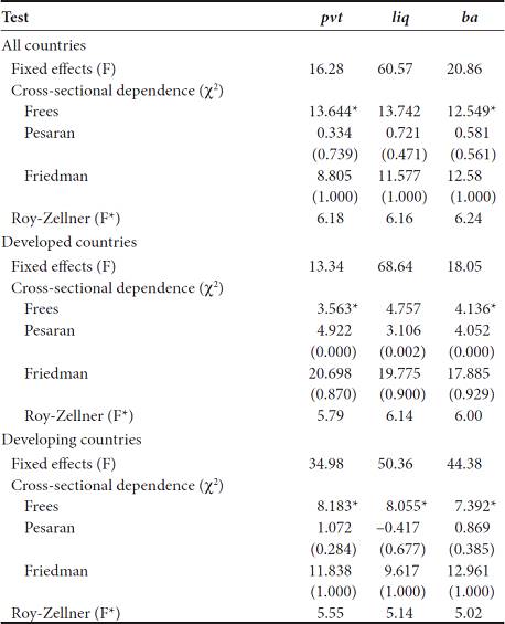
Note: * Indicate statistical significance at less than 10%.
Source: Authors’ calculation.
4.1. Ordinary least squares
Table 2(A) displays the results of the OLS estimation of the effects of inflation on financial variables11. Given that we rejected the null hypothesis of constant variance with the Breusch-Pagan/Cook-Weisberg test for heteroskedasticity12, we obtained the White’s heteroskedasticity-corrected t-values and the corresponding p-values. In the specifications where pvt, liq, and ba are dependent variables, inflation rates exert a negative influence significant at more than 95%. All control variables have the expected sign, although gov and rev are usually insignificant. To understand the economic importance of the estimates, a basic experiment shows that an increase in inflation rates of 8.3% (median value) can cause a fall of 3.4% in private credit, 4.9% in liquid liabilities and 4.5% in bank assets13.
Table 2: OLS, POLS and FE estimation of the effects of inflation on financial intermediary performance

Note: For the OLS estimation, period averages were used (1980-2010). Variable y is initial income per capita. Standard errors are White’s heteroske-dasticity-corrected. POLS is pooled OLS estimation, whereas fe is fixed-effects estimation. In this case, robust standard errors are provided.
Source: Authors’ calculation.
In Table 2(B) we report the POLS estimators. The variable of interest presents clearly negative and statistically significant effects on private credit, liquid liabilities and bank assets. Nonetheless, with respect to the OLS estimators the coefficients of inflation are smaller. In general, the control variables also maintain the same signs as in the previous estimation. The control variables presenting adequate and statistically significant coefficients are still income per capita and education. Interestingly, rev became significant in private credit, liquid liabilities and bank assets, suggesting that an increase in political instability tends to reduce the performance of financial intermediaries in the long run. Thirdly, Table 2(C) exhibits the fixed effects estimators. In comparison to the other two methods, inflation remains negative but statistically insignificant suggesting no influence on financial development14. Although income per capita and education are positive and highly significant in most cases, gov and rev switched signs, generally contradicting theoretical and empirical findings.
Finally, for POLS and fixed effects we report the coefficients of inflation by country group. With regard to the first method, it is observed that inflation levels are consistently insignificant for all the financial variables, although they keep the expected negative sign. On the other hand, price increases are statistically significant at the 1% level for the first three financial variables in developing countries. By the same token, a similar pattern is seen when we disaggregate the data and apply the fixed effects method. For developed countries, there is no empirical evidence of the influence of inflation using any of the three financial indicators. Contrarily, the evidence is statistically strong for less-developed economies.
In summary, by utilizing a variety of linear regression models we have initially proved the empirical existence of the inflation-finance nexus mainly in developing countries. Preliminarily, we can infer that the statistically significant relationship between inflation and finance observed in the full sample of countries is due to the behavior of developing countries, given that the relationship is insignificant for developed countries.
4.2. Standard quantile regressions
Until now we have discussed the effects of inflation rates on financial variables based on ordinary least squares, pooled OLS and fixed effects estimators. But the main purpose of this paper is to assess the inflation-finance link with quantile regressions to verify how the negative relationship varies along the conditional finance distribution. Henceforth we only report inflation coefficients.
Table 3 shows the estimation results of the three financial variables using the whole sample of countries. In the case of private credit, it is observed that the effects of inflation are statistically significant in the lower and upper part of the distribution (it is significant in the 70th quantile at the 5% level). The results point out that an increase of 1% in inflation leads to a fall between 1 and 2.3% in private credit depending on the quantile. Second, in the equation for liq inflation is significant up to the 50th quantile at the 1% level, suggesting that the adverse effects of inflation rates are concentrated in the lower parts of the conditional liquid liabilities distribution. The value of coefficients goes from -1.1 to -3.9%. Third, the results regarding bank assets are similar to private credit, in the sense that the statistically significant negative effects of inflation are concentrated in the lower parts of the distribution and in the 70th quantile.
Table 3: Effects of inflation on the conditional finance distribution without controlling for country fixed effects: All countries
Note: p-values are in parentheses. Due to lack of data, Chile was excluded from liq and ba, and Germany and Venezuela from ba. *, ** and *** indicate statistical significance at 1, 5, and 10%, respectively. Bootstrapped standard errors.
Source: Authors’ calculation.
As shown in Table 4, the estimation for developed countries produces bigger coefficients. Apparently, inflation is very damaging to financial sector performance in developed countries, and possibly it is the case because authorities in developed countries have been able to control inflation for a long period of time, and a sudden or unexpected increase in inflation could provoke a sharp deterioration in financial variables. Another explanation is that the activity of financial intermediaries is strongly related to output, thus permeating the behavior of economic agents. Depending on the level of inflation, private sector bank credit would fall between 66.3 and 91%; liquid liabilities between 56.7 and 116%; bank assets between 46 and 116%. We also observe that the effects of inflation are grouped around the lower parts of the distribution, precisely because inflation in high-income countries has been kept controlled for a long period of time.
Table 4: Effects of inflation on the conditional finance distribution without controlling for country fixed effects: Developed countries
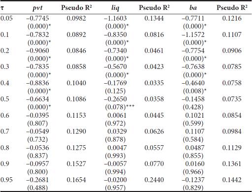
Note: p-values are in parentheses. Due to lack of data, Germany was excluded from ba. * and *** indicate statistical significance at 1 and 10%, respectively. Bootstrapped standard errors.
Source: Authors’ calculation.
The story for developing countries is rather different, as presented in Table 5. Coefficient estimates are more heterogeneous with respect to the preceding results. In relation to private credit, inflation effects concentrate around the middle part of the conditional distribution, and for liquid liabilities, in the first half of the distribution. For the case of bank assets, they were significant in the 40th and 50th quantiles. An increase of 1% in inflation would provoke a drop between 0.6 and 0.7% in private credit. The same small coefficients are obtained for liquid liabilities with values ranging from -0.6 to -1.8%. Thus, these results indicate evidence on the relationship between the level of inflation and finance in developing countries. Considering that inflation rates have been higher in those countries, the negative effects oscillate around the middle part of the distribution.
Table 5: Effects of inflation on the conditional finance distribution without controlling for country fixed effects: Developing countries

Note: p-values are in parentheses. Due to lack of data, Chile was excluded from liq and ba, and Venezuela from ba. *, ** and *** indicate statistical significance at 1, 5, and 10%, respectively. Bootstrapped standard errors.
Source: Authors’ calculation.
In a few words, our QR estimations confirm some theoretical predictions. The estimations suggest a negative, nonlinear relationship between finance and inflation, which is stronger in the lower and middle parts of the conditional finance distribution. However, we have to remove country fixed effects to show precisely where the significant effects lie on the conditional distribution. We should expect that at higher inflation rates the adverse impact on finance should be stronger.
4.3. Fixed-effects quantile regressions
In this subsection we discuss the results of the estimation by controlling for country fixed effects. Overall, we found fewer significant quantiles than before, they are less heterogeneous, and the few significant ones were pushed up along the conditional finance distribution, i.e., they moved up to the upper tail of the distribution. Andini and Andini (2014, p. 8) offer a plausible explanation for this comportment: Certain effects originating in other quantiles of the conditional finance distribution produce the dominant effect of inflation over finance in the lower tail of the distribution. Another central outcome is that, based on our preferred QR method, we did not ascertain strong evidence on the inflation-finance relationship in developed economies, as we will discuss below.
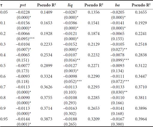
Table 6 exhibits results considering the full sample of countries. Inflation rates impact private sector credit on the upper tail of the distribution at least at the 5% level of statistical significance. For liquid liabilities the effects are meaningful from the 30th quantile onwards and for bank assets since the 60th quantile. Therefore, after eliminating country fixed effects the results look more precise in the sense that at the higher quantiles of the conditional finance distribution inflation exerts stronger negative effects.
Table 6: Effects of inflation on the conditional finance distribution, controlling for country fixed effects: All countries

Note: p-values are in parentheses. Due to lack of data, Chile was excluded from liq and ba, and Germany and Venezuela from ba. * and ** indicate statistical significance at 1 and 5%, respectively. Bootstrapped standard errors.
Source: Authors’ calculation.
In regard to the subsamples of countries, there are sharp differences in comparison to the QR estimates -or even the fe estimates, as revealed by Tables 7 and 8‒. For developed economies, inflation appears to affect only pvt in the 95th quantile at the 10% significance level (statistically weakly) and liq in the 20th quantile at the 10% significance level. In fact, these results are more consistent with the low levels of inflation rates experienced by developed countries in the past 30 years. That is one reason why one would expect that inflation rates had a minor effect on advanced financial intermediaries. By comparison and consistent with the results shown in Table 2, the impact of inflation in less-developed economies varies widely because we observe more statistically significant quantiles in the regressions. For private credit, inflation rates are highly significant after the 80th quantile; for liquid liabilities, most quantiles have at least 5% significance level after the 20th quantile; and for bank assets, the acceptable quantiles are only the 30th, 50th and 70th. Overall, we can argue that the higher the inflation rates, the lower the level of financial sector performance and those effects are more meaningful in developing economies. It should be noted as well that the estimations for the full sample of countries are mainly driven by the impact of inflation in developing countries, given that the influence in developed countries is rather null.
Table 7: Effects of inflation on the conditional finance distribution, controlling for country fixed effects: Developed countries

Note: p-values are in parentheses. Due to lack of data, Germany was excluded from ba. *** indicate statistical significance at 10%. Bootstrapped standard errors.
Source: Authors’ calculation.
Table 8: Effects of inflation on the conditional finance distribution, controlling for country fixed effects: Developing countries
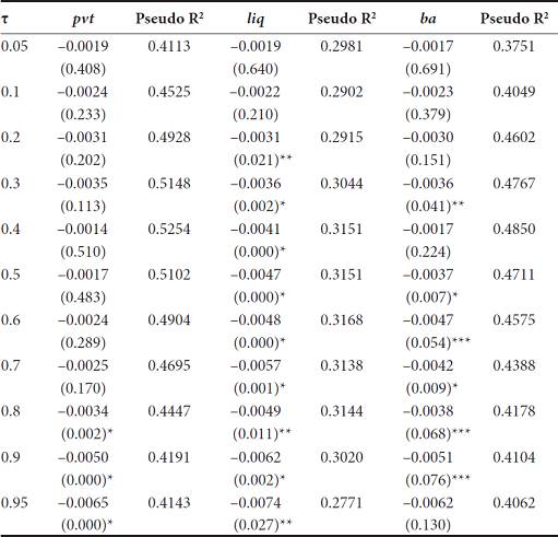
Note: p-values are in parentheses. Due to lack of data, Chile was excluded from liq and ba, and Venezuela from ba. *, ** and *** indicate statistical significance at 1, 5 and 10%, respectively. Bootstrapped standard errors.
Source: Authors’ calculation.
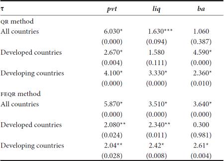
4.4. Inter-quantile tests
Table 8 reports the results of the inter-quantile tests as proposed by Koenker and Bassett (1978). We test the null hypothesis that β0.5 ≠ β0.10 ≠ β0.20 ... ≠ β0.95, which corresponds to the estimated quantiles in the standard and fixed effects quantile regressions. When we reject the null hypotheses at a minimum of 5% significance level, then the coefficients of the estimated quantiles are valid. From Table 9 we can infer that for private credit all the quantiles are different from each other in the QR and FEQR regressions. For liquid liabilities, the standard quantile regressions are invalid in the case of the full sample and developed countries. And with respect to bank assets, the results are mixed. Under the FEQR technique, the estimations for developed countries are invalid.
4.5. Additional results including legal institutions
So far we have explored the influence of macroeconomic variables on the performance of the financial sector. However, it is worth analyzing the inclusion of institutional development in our empirical model. In fact, many studies prove that legal protection of rights and the enforcement of contracts enhance financial development in the long run (see, for instance, La Porta et al., 1998; Billmeier and Mass, 2009). Miletkov and Wintoki (2012, p. 651) explain that risks and uncertainty are lowered when countries have strong legal institutions, and that their societies begin to receive the benefits of property right protection when its maintenance costs have been surpassed.
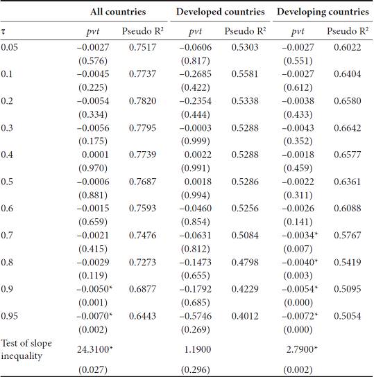
As in Miletkov and Wintoki (2012) and the references therein, we use the popular Legal Structure and Security of Property Rights Index from the Economic Freedom of the World. This index ranges from 0 to 10, where 0 is the lowest value and 10 is the highest. The index is an average of the following components: Judicial independence, Impartial courts, Protection of property rights, Military interference in rule of law and politics, Integrity of the legal system, Legal enforcement of contracts, Regulatory costs of the sale of real property, Reliability of police and Business costs of crime. Given that the index does not cover all countries, our sample was reduced to 46 developing countries. Since the available years for the latest index are 1980, 1985, 1990, 1995 and 2000-2014, we used averages for the missing years assuming that institutions do not change significantly in the short run. In order to save space we only report the results for our main indicator of financial development (i.e., bank credit to the private sector) and the fixed-effects quantile regressions15.
Table 10 presents the estimation results adding the index of legal institutions. In general, we obtain the same results as in the previous subsection: There is a persistent negative effect of inflation on financial sector development even after controlling for legal institutions. For the whole sample of countries and developing countries, the effects are statistically significant in the upper quantiles. In the case of developed countries, we can see that the effects of price increases are statistically insignificant in all quantiles. The lack of evidence for developed countries is confirmed as well by the test of slope inequality, as shown at the bottom of Table 10.
Table 10: Effects of inflation on the conditional finance distribution, controlling for country fixed effects and legal institutions
Note: p-values are in parentheses. Due to lack of data on legal institutions, the following developing countries were excluded from the sample: Belize, Fiji, Gambia, Lesotho, Nepal, Rwanda, Sudan and Swaziland. * indicates statistical significance at 1%. Bootstrapped standard errors are reported.
Source: Authors’ calculation.
4.5. Discussion
In a stable macroeconomic environment accompanied by adequate supervision and regulation, financial intermediaries can be powerful enough to enhance economic output in the long run and, as a corollary, improve the standard of living of people. With the estimations shown in this section, we have found evidence of an inverse and nonlinear relationship between finance and inflation in 84 developed and developing countries. In all of the statistically significant QR and FEQR estimations, the inflation was persistently negative. Based on our preferred FEQR estimations and with some caution about the causality issue, we observe that inflation rates reduce the level of financial development in the upper quantiles of the distribution, principally in developing countries where the effect is stronger. We did not obtain robust empirical evidence for developed economies.
With respect to lack of evidence in developed economies, one explanation is that in those countries inflation rates have been kept controlled for a long period of time and they have also enjoyed of a relatively stable macroeconomic atmosphere. On the other hand, these results agree with the literature that has revealed weak evidence on the finance-growth and finance-inflation link in high-income countries. De Gregorio and Guidotti (1995) add bank credit to the private sector in a sample of 98 countries for the 1960-1985 period. Even if they discover a positive effect of the proxy of financial development on growth, it is stronger for developing countries only. Huang and Li (2009) study the finance-growth association in a sample of 71 high- and low-income countries with cross-section IV threshold regressions. Although they determine that the association is nonlinear, the impact is more prominent for low-income countries. With respect to inflation, Beck, Lundberg, and Majnoni (2006) inspect a panel of 63 countries during the period 1960-1997 with which they found solid evidence of a positive interaction between finance and inflation volatility in low- and middle-income countries. On the contrary, their econometric analysis did not provide any robust effect in countries with well-developed financial markets. The logic behind such results is that in developed countries most intermediary development happens outside the banking system, which diminishes the efficacy of monetary policy and thereby the effects of shocks of consumer prices.
5. Conclusions
The finance-inflation nexus has been studied intensively in the last two decades with different econometric approaches of time series and cross-section and panel data. Even though the literature has determined that there exists a negative, nonlinear association between inflation and financial intermediary development, previous studies did not examine it in more detail. In this paper we investigated the link using standard and fixed-effects quantile regressions. We applied different econometric techniques (i.e., OLS, POLS, FE, QR and FEQR) to a panel data of 84 countries for the 1980-2010 period.
Two important features emerge from this investigation that confirm empirically the inverse, nonlinear association mentioned before. First, the estimated coefficients show a high degree of heterogeneity at different quantiles of the conditional finance distribution. And second, the influence of inflation on financial intermediaries is more heterogeneous in developing countries than in developed countries. According to our preferred FEQR estimator, for the former group of countries the effects of inflation are smaller than in developed economies. However, the impact of price increases in developed countries was mostly statistically insignificant. And second, the finance-inflation nexus is stronger in the upper tail of the distribution in developing countries, meaning that inflation rates affect more the higher levels of financial development.
There are some policy implications arising from our research. The first implication is that governments and central banks should continue fighting against inflation with an adequate monetary policy in order to maintain macroeconomic stability. Another implication is that authorities should pay attention to non-linear effects of inflation on financial sector development and thus on economic growth. In fact, not taking into account non-linearities and thresholds “(...) can give a misleading impression that inflation must become quite high before its cumulative effects become important” (Ndou and Gumata, 2017, p. 291). As a consequence, if inflation is low and stable investors and financial market participants can take better long-term investment decisions. As inferred by the empirical evidence on finance and growth, better investments in terms of efficiency increase productivity and long-run economic growth.
Future research will help us understand better the finance-inflation nexus in both developed and developing countries. With the econometric technique of fixed-effects quantile regressions we found a weak relationship in developed economies, an area that deserves more attention. A possible research extension would be to use different time periods or period averages in order to find a stronger relationship. Moreover, it could be possible to divide the sample into three income groups (high, middle and low) to try to understand better how inflation behaves within each of them. In any case, the authorities should continue focusing on keeping low inflation because when it is high and uncertain, it erodes all economic activities and in the end the living standard of all people.


