SciELO - Scientific Electronic Library Online

 
vol.76 número299Government financial regulation and growth índice de autoresíndice de assuntospesquisa de artigos
Home Pagelista alfabética de periódicos  

Serviços Personalizados

Journal

Artigo

Indicadores

Links relacionados

  • Não possue artigos similaresSimilares em SciELO

Compartilhar


Investigación económica

versão impressa ISSN 0185-1667

Inv. Econ vol.76 no.299 Ciudad de México Jan./Mar. 2017


Artículo para el debate científico

The nonlinear relation between biofuels and food prices

Salvador Cruz Akéa 

a Escuela Superior de Economía of the Instituto Politécnico Nacional (IPN, Mexico). Correspondence: salvador.ake22@gmail.com.


Abstract:

This paper analyzes the relationship between the production of agricultural foods (cereals and vegetable oils) and the production of energy by using food. The observed increase in economic activities that use energy has had an impulse in the energy industry with higher prices. These prices make profitable the biofuel production, and this encourage the use of cereals for biofuel production, affecting the whole food chain. This research demonstrates that the agricultural foods and energy production system has been in place at least since 2000 and that it remains active or latent depending on the price of energetics. The paper also shows that the temperature variations do not lead the system to an adjustment. To do, this research uses the econometric technique of Dynamic Conditional Correlation, and a new tool, phase synchronization. The use of the latter avoid making assumptions on the distribution or stability of the involved variables.

Keywords: Dynamic Conditional Correlation; phase synchronization; energy prices; agricultural foods

Keywords: Energy prices; biofuels; time series models; agricultural foods

Resumen:

Este trabajo analiza la relación entre la producción de alimentos y la producción de energía mediante el uso de alimentos. El aumento observado en las actividades económicas que utilizan energía ha tenido un impulso en la industria energética con precios más altos. Estos precios hacen rentable la producción de biocombustibles, lo que promueve el uso de cereales aceitosos para la producción de biocombustibles, afectando a toda la cadena alimentaria. Esta investigación demuestra que el sistema de alimentos y energía ha estado en vigor al menos desde el 2000 y que permanece activo o latente dependiendo del precio de la energía. El documento también muestra que las variaciones de temperatura no llevan al sistema a un ajuste. Para ello, esta investigación utiliza la técnica econométrica de correlación condicional dinámica y una nueva herramienta, la sincronización de fase. El uso de esta última evita hacer suposiciones sobre la distribución o la estabilidad de las variables involucradas.

Palabras clave: correlación condicional dinámica; sincronización de fase; precios de energía; alimentos agrícolas

Palabras clave: precios de la energía; biocombustibles; modelos de series de tiempo; alimentos

JEL Classification: C22; C63; O13.

Clasificación JEL: C22; C63; O13.

Introduction

The fall in the oil prices in 2014 decresed dramatically the average price of energy measured thruogh the Fuel Energy Index1 (FEI). A couple of years before, the Food Index2 (FI) began its declination, briefly interrupted by an increase from March 2016 until August 2016, almost on the same date and with a similar pattern. Morever, the Fat and Oil Index3 (FOI) began its downward movement in the same since 2014. With these facts, it seems that there is not a direct relation between the agricultural foods and the energy prices or the oily cereals and energy prices. In fact, some recent studies as those published by Zhang et al. (2010), Gilbert (2010), Ajanovic (2011), and Qiu et al. (2012) provide empirical evidence of a no linear relationship between food and energy prices.

On the other hand, other studies as those from Kristoufek, Janda, and Zilberman (2013), Vacha et al. (2013) and Nazlioglu, Erdem, and Soytas (2013) found nonlinear relations among the energy, the biofuels, and the food prices. Evenin non-completely developed countries as Turkey, Nazlioglu and Soytas (2011) obtained an alike conclusion. In a similar direction, the studies from Harri, Nal-ley, and Hudson (2009), Ciaian and d’Artis (2011b) or Pokrivčák and Rajčániová (2011) found a long run relation by using cointegration analysis among the prices of some oily cereals, biofuels, and oil prices.

This paper will show that there is a non-linear relation between the yields (returns or growth rates) of the food prices, the biofuels usage, the economic activity, and the energy prices. The main claim of this paper is that the global economic activity that uses energy causes the rise in the prices of fuels (biofuels and liquid fuels4 as substitute goods) and the food (as a competitive good with biofuels). The mechanism begins with those economic activity that need fuel. The vast majority of the business requires machines or transport, which is closely related to the fuel usage.

When there is a business cycle expansion, the price of liquid fuels (closely related to the cost of energy and crude oil) rises, making profitable the production of biofuels. The economic expansion also makes that a greater part of the population consumes more and better basic goods as food (raises the cereals and meat consumption) making the food more expensive because of the demand rising and the increase in the production costs (transport and fertilizers).

The size of temperature variation (measured in the mean world temperature, MWT, variable) were part of the econometric model, but they were statistically non-significative. This variable was kept for the phase synchronization analysis althuogh only presented a single and not related cycle. Also the prices of wheat, corn and oil were redundant to the econometric model (with the associated econometric problems) because there is a variable resuming their prices (Food Index), so they were also discarded from the analysis.

This investigation will use a multi-varied student t distribution of a Dynamic Conditional Correlation model (DCC) and a generalized extreme value distribution for the variance process. Also, this paper contributes to the analysis of the long-run relation among those variables by detecting the number of cycles and the time periods in which they are intimately related (hooked), this is a result of a phase synchronization study.

With the aim of explaining the puzzle of the non-constant relation between these prices, authors as Saitone, Sexton, and Sexton (2008), Ciaian and d’Artis (2011a), and De Gorter and Just (2009) proposed theoretical models that attempt to explain the effect of the energy prices on other relevant variables. In general, the models take into account the role of biofuels (as a competitive product), the land (as a resource for the biofuel) and the food (as substitute use for the land), among other distinctive features that distinguish one model from other. As a general result, this kind of works proved that the use of biofuels would not threaten the food production only if the crops aimed for biofuels come from marginal lands, the producers use second generation technology5 for generating the fuel, or if they use new lands for agriculture. If this is the case, several studies as those from Von Blottnitz and Curran (2007), Pimentel and Patzek (2008) or Hill et al. (2006) point out the fact that the biofuels loose their alleged carbon neutrality6.

A step forward in that kind of models is the use of Computable General Equilibrium models as those proposed by Kretschmer and Peterson (2010), Birur, Hertel, and Tyner (2008) or Hayes et al. (2009). This kind of models gives a very useful theoretical knowledge of the problem, its transmission channels and the possible sources of non-linearity; however, they offer a poor predictive power because of their need for calibration and lack of adaptative response when the economic conditions change.

To overcome the problems of adaptation to the variable economic conditions, researchers as Busse, Brümmer, and Ihle (2012) propose non-linear tools as the Markov chain models to explain the regime shift in the relation of the studied variables. Another example of this kind of proposals is the work of Balcombe and Rapsomanikis (2008), they proposed a non-linear Vector Error Correction model (VEC) to explain deviations of the analyzed variables from a long run equilibrium. For their part, Du, Cindy, and Hayes (2011) proposed a similar approach, focused on volatility, using an Stochastich Volatility Merton Jump model (SVMJ).

On the other hand, Escobar et al. (2009) calculated that the biofuels production is only profitable in the European Union when the oil reaches 75 to 80 USD per barrel. They also fund that bioethanol and biodiesel are profitable when the crude oil reaches 90 to 100 USD per barrel. They extended their analysis to the second generation biofuels finding that biodiesel would be profitable only after the crude oil reaches 150 to 160 USD per barrel.

For the United States case, the break-even point for an average bioethanol producers is near to a price of 40 to 50 USD per barrel of crude oil. By their side, an average bioethanol Brazilian producer can be profitable when the international price of the crude oil is near to 30 to 35 USD per barrel and in 60 USD for biofuels derived from vegetable oils.

Whit this information from the current state of the art at hand, this paper states two main contentions: First, the transmission mechanism between the yields of economic activity, the crude oil price, the biofuels price and the food prices (including oilseeds) is nonlinear, nonnormal and changes as the variables evolve. In particular, the correlation of their variances increases as the variance or the mean yield increases. Second, the conditional and nonlinear transmission mechanism present in the yields results in a long run dependence between the analyzed variables. This long-run relation creates economic cycles that can be “hooked” for specific and measurable time intervals that reflect “temporary common trends” for the variables.

This research proposes a two-fold analysis. The first stage consists of a non-normal Dynamic Conditional Correlation for the yields (returns or growth rates) of the studied variables. The second stage consists of a phase synchronization analysis to the levels of the same variables. For simplicity, we define the studied variables in Table 1 and show its general behavior in Figure 1.

Table 1: List of studied variables and their sources 

Note: All of them are available from <https://www.quandl.com/>.

Source: Own elaboration in R (R Core Team, 2015).

Figure 1: General behavior of the analyzed variables 

In the next section, this research briefly explains the usage and limits of the dcc model and show the results of its application to the analysis of the volatility transmission between the yields of economic activity, the yields in the prices of the liquid fuel, the biofuel prices and the food yields. In the third section, a similar scheme is used to explain the long run relation and its time duration of the levels of those variables by using a phase synchronization methodology. This method work without making any assumptions on the distribution or stability properties of the time series. Finally, the paper resumes its findings and recommendations.

Dynamic Conditional Correlation model

The Dynamic Conditional Correlation model, DCC, is a multivariate Generalized Autoregressive Conditional Heteroskedasticity model (GARCH) capable of calculating time-varying covariances for the variables in the studied system, as stated in Engle and Sheppard (2001). The DCC was developed by Engle (2002) as an enhancement of the Baba-Engle-Kraft-Kroner model (BEKK), initially proposed Baba et al. (1990), but developed in Engle and Kroner (1995). This model has the shortcoming of needing k 4 parameters to capture all the possible dependence within the model. This makes it unpractical for models above or equal to three variables. Because of that, the model is usually calculated using the principal diagonal of the variance-covariance matrix, thus, it requires the calculation of k 2 parameters.

The DCC model proposed in this paper assumes that the yields, y it , of all the used variables follow a conditionally multivariate student t distribution with zero mean and time-dependent variance-covariance matrix. Thus, the representation of the system y t , is:

In this case, D t is the square diagonal matrix of time-varying standard deviations from the univariate generalized extreme value distribution (sgev) for each EGARCH models. Nelson and Cao (1992) supposed for each variable, hit that:

where sgev (γ ,σ, χ) are the parameters of location, skew, and shape, respectively, for the generalize extreme value distribution of the innovations in each yield.

To express the dynamic correlation structure, the model postulates that it depends on the squared errors of the system εtεt', and the past values of the dynamic correlation structure.

In this case, Q- is the unconditional covariance of the model’s standardized residual. This gives, as a result, a parallelism of the dynamic correlation equation of the whole system with the single GARCH process.

In their papers, Engle and Sheppard (2001) and Engle (2002) demonstrate the estimation procedure for the parameters and their consistency, so all the common set of hypothesis tests can be performed to check if the system’s residuals are white. If after performing those tests, the residuals result to be white noise (independent and jointly normal), then the model explain the phenomena and so, it took out all the dependence structures of the system.

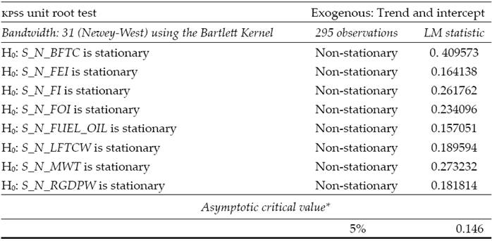
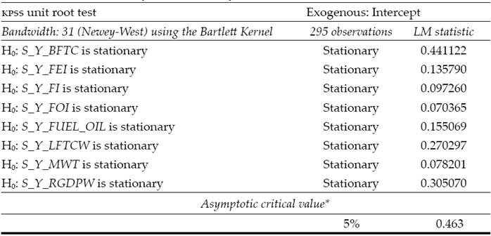
Now, after briefly explaining the dcc model, we present the results of the dcc model applied to the proposed system. Table 2 shows the results of the Kwiatkowski-Phillips-Schmidt-Shin test (KPSS) (Kwiatkowski et al., 1992) for the yields of the selected variables7 and Figure 2 shows the general behavior of the yields of the selected variables.

Table 2: KPSS tests for the selected variables 

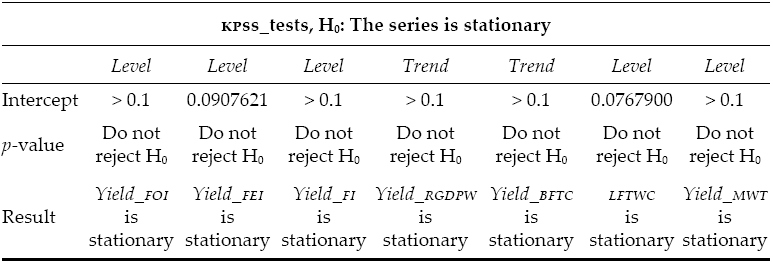
Source: Own elaboration with tseries package (Trapletti, Hornik, and LeBaron, 2016) form (R Core Team, 2015).

Source: Own elaboration in R (R Core Team, 2015).

Figure 2: General behavior of the yields of the analyzed variables 

As the reader may see, the FI, FEI and FOI index yields have very similar behavior. They are also heavily related to the yield of the RGDPW. On the other hand, there seems to be a likelihood between changes in the abnormalities in the MWT and the use of BFTC, but the relation is statistically nonsignificant.

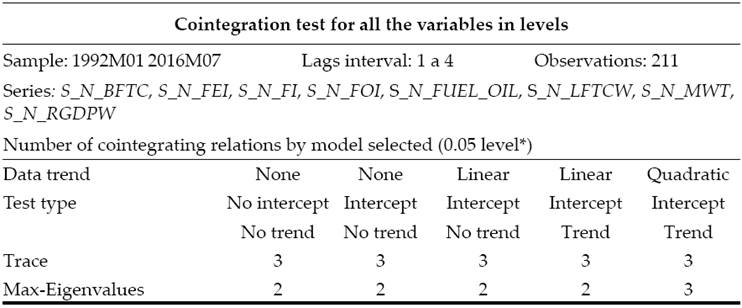
To properly compare this work with those cited in the introduction, the paper shows a Vector Autoregressive model (VAR) in Table 3. In this table, the reader may see that there is no evidence for supporting the hypothesis of linear dependence between the yields of Fats and Oils, Energy or Food indexes. In order to maintain the article length acceptable, the paper does not present the impulse response graphs, nor the residuals test or the variance decomposition graph for the model. As the reader can anticipate, they only show almost non-related patterns and nonlinearity problems, as a significant part of the previous authors showed.

Table 3: VAR model for the Fats and Oils, Energy and Food indexes 

Source: Own elaboration using the vars package (Pfaff, 2008) in R.

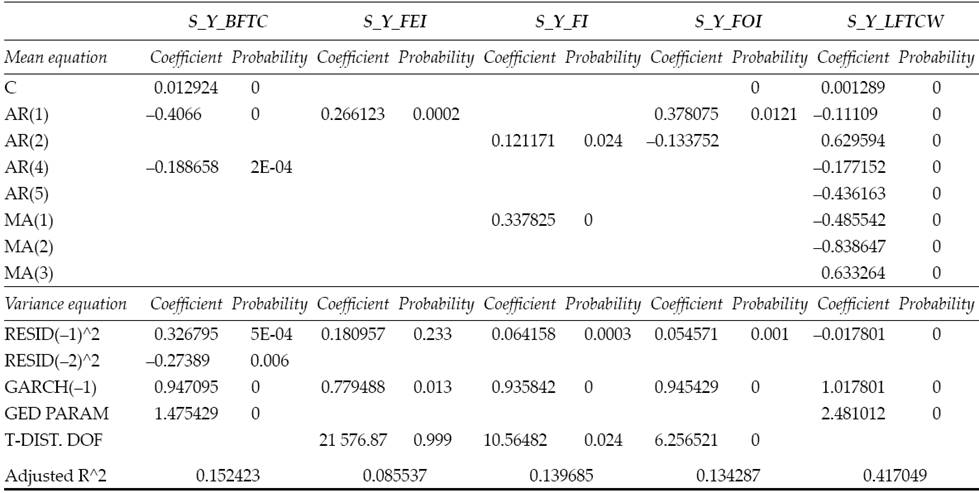
In an attempt to catch the nonlinear relations within the proposed system, the paper exhibits a DCC model, done using the rugarch (Ghalanos, 2015a) and rmgarch (Ghalanos, 2015b) with R packages. The dcc model appears in Table 4.

Table 4: DCC model for the proposed system 

Source: Own elaboration with the rugarch (Ghalanos, 2015a) and rmgarch (Ghalanos, 2015b) packages for R.

The main result of this part of the article is showed in Figure 3. There, the reader may see the way in which the correlations among the variables change over the time, peaking during 2008 (when the food prices rose sharply) and getting down to the growth of the world’s GDP stopped and recovered as the world’s economy gets recovered.

Source: Own elaboration with R.

Figure 3: Estimated conditional correlation for the DCC model 

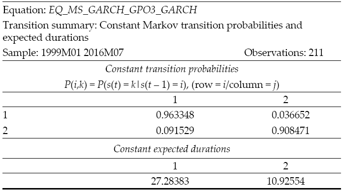
Figure 3 also showed the “Markov switching” feature described by other authors. In fact, the graph shows correlations swinging into a large but related correlation spans. This related correlations spans are also the footprint of the volatility clusters and other nonlinearities registered in other works. This characteristic also may explain the nonnormal distribution that affects the econometrics calculations given by previous works.

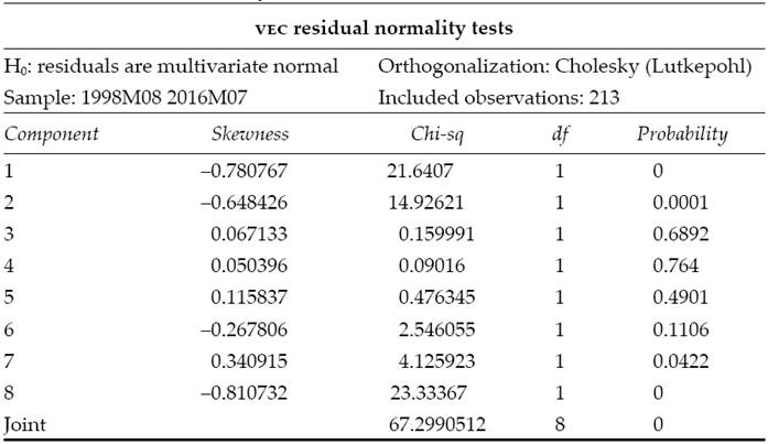
Unfortunately, the examined system is heavily nonnormal and even though the dcc model takes out the first and second order dependence structures, there are higher order dependencies that prevent the model’s residuals from reaching normality nor independence. In Table 5 and Table 6, we show the joint normality test (Henze and Zirkler, 1990) and the Brock-Scheinkman-Dechert (BDS) test (Broock, Scheinkman, and Dechert, 1996) for the model residuals.

Table 5: Multivariate normality test for the model’s residuals 

Source: Own elaboration using (Korkmaz, Goksuluk, and Zararsiz, 2014) MVN package from R.

Table 6: BDS test for DCC model’s residuals 

Source: Own elaboration with (Wuertz, 2013) fNonlinear package from R.

After performing all the necessary tests to the dcc model, the reader may see that it does not suffice to get white noise residuals. Nevertheless, the model captured the first and second order dependencies from the specified system and helped us to prove the first part of the paper’s arguments:

  • There are nonlinearities in the system, and the yields cause them in the World’s GDP, they pass to the Fuel and Energy and Fat and Oil indexes and then to the Food Index.

  • The volatility spillover occurred when the whole system becomes stressed.

Now, the paper presents a phase synchronization analysis to the levels of the same variables to test similar relations in original series without making any assumptions on the distribution or the stability of each time series.

Phase synchronization

The synchronization is used to assess the similarity between two nondeterministic systems. Christian Huygens created the concept when he discovered that two pendulum clocks tend to synchronization if they were on the same surface. This type of synchronization was called “phase synchronization” and originated the coupled oscillators analysis. The main characteristic of this kind of systems is that no matter how wide the pendulum may be, or if they are of a different size, the will fulfill their cycle at the same time.

This type of phenomenological analysis can be used to analyze systems that hardly meet the standard assumptions of independence and joint normality that are common in the time series analysis, as those of this paper. The first step to perform this analysis is to normalize (get into a similar scale) all the time series. For this purpose, all the time series are divided by their maximum, the result of this procedure appears in Figure 4.

Source: Own elaboration with Fortran and GNUplot.

Figure 4: Normalization for the main Food and Energy indexes 

The main objective of using this kind of methodology is to the obtain the system dynamics and to get the time periods in which the cycles of the series had the same duration and therefore are synchronized. It is important to mention that this synchronization does not mean that the dynamics of the series are in the same direction, it only implies that the cycles are of the same length. As the reader may see in Figure 4 the dynamics of the FEI, FI, and FOI indexes seem to be synchronized.

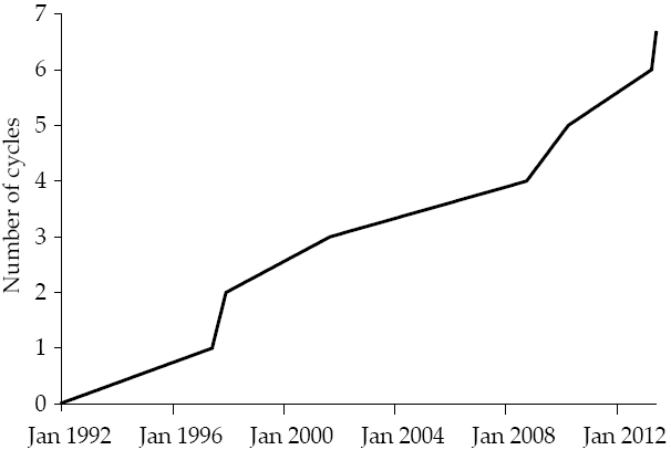
The synchronization analysis continues with the definition of the cycles of the smoothed time series of the first derivative. The period in which the smoothed series presents two sign changes defines the entire cycle8. In the case of random time series, the duration of the cycles may be different for each cycle, so the first step is to determine how many cycles presents each time series. The article shows this calculation for all the time series in Table 7.

Table 7: Number of cycles for the smoothed selected variables 

Source: Own elaboration in Fortran.

The above table provides empirical evidence of the visual analysis stated with Figure 4. Table 7 provides empirical evidence that FEI, FI, LFTWC and FOI present similar trajectories, with almost equal number of cycles (FOI is faster and LFTWC slower).

Figure 5 shows the time in which each variable completes its cycles. It is re-markable that in October 2008, the FEI, FI, and FOI indexes ended their cycles in the same time (LFTWC did it a few months earlier). A similar phenomenon (but not so accurate) occurred in 2012 for FEI and FI, with FI and FOI in 2010, and with FEI and FOI in 2014.

Source: Own elaboration with Fortran and Excel.

Figure 5: Short run cycles for the selected variables 

It is also remarkable that FEI and FI indexes have a very similar number of cycles, but their amplitude (distance from peak to peak) in the 2008 cycle were different. In this case, the FEI index has an amplitude of 212.48 and for fi is just 83.85 while FOI has a similar 86.79, this is an empirical evidence of the series being “hooked” in stress periods and may remain independent under other conditions. The goodness of this kind of analysis is that it seeks synchronization in the dynamics of the series, this is the generated number of cycles not in the amplitude.

Once the number of periods is known, one may calculate the phase for each variable. The phase is the amount in which each oscillatory cycle increases 2π. It can be calculated using:

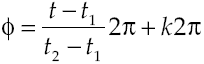
where k is a counter for the cycles9. The only change will be the number of the cycle, k. Applying the phase equation to the analyzed data, we obtained a phase graph like the one obtained for the Food Index and showed in Figure 6.

Source: Own elaboration with Fortran and GNUPLOT.

Figure 6: Phase for the Food Index 

The empirical analysis revealed so far by the series only refers to its individual properties (number of cycles and its amplitude); however, to determine if there is synchrony between the dynamics of these variables is necessary to calculate the phase differential. If the phase differential is constant, then both series present a phase synchronization, this is:

The constant difference between the phase of two-time series implies that the duration of the cycles is the same for both, although their respective intensity (amplitude) is not. In Figure 7 we present a differential analysis for the FEI and FI time series. The research uses this time series as an example because those series presented the same number of cycles. In Figure 7, the reader can observe that the phase difference is almost constant, with a first synchronization period from January 1992 to August 1998, and a second term from September 1998 to March 2008 when the series lost their synchrony.

Source: Own elaboration with Fortran and GNUplot

Figure 7: Phase differential for Fuel an Energy Index 

Figure 8 shows a resume of the phase synchronization of the selected variables. Here, the reader can observe that the whole system presents an almost constant phase synchronization since 2000 (when the biofuels became popular)10. The reader also may see that the phase synchronization is partially lost when the world’s economy faces a crisis. The loss of synchronization is acuter in the Liquid Fuel Total World Consumption and Biofuel Consumption.

Source: Own elaboration with Fortran and GNUplot.

Figure 8: Resume for phase synchronization for selected variables 

It is also remarkable the fact that is the Liquid Fuels Total World Consumption, and thus the economic growth the leading factor of the system and not the anomalies in the global mean temperature, MWT. The lack of phase synchronization of the anomalies of the global average temperature indicates that the shock does not come from the global agricultural sector (it is not so decisive for the Food Index if there are some anomalies in some parts of the world). A possible explanation for that behavior is that a bad agricultural season in a country is partially offset by a good season elsewhere, also because the market prices control the amount of resources used for energy and food as the rest of the economy plump or fall.

Conclusions

This paper gave empirical evidence of the existence of an economic system that includes the Biofuel Total Consumption, BFTC; the Liquid Fuels Total World Consumption, LFTWC; the Food Index, FI); the Fuel Energy Index, FEI, and the Real Gross Domestic Product for the World, RGDPW, by using a DCC model and the phase synchronization methodology.

The paper also showed with the DCC model that is the RGDPW, and not the MWT the variable that unchains the movements of the whole system. The transmission mechanism starts with the RGDPW pushing up the LFTWC and thus its prices (FEI). When the prices are high enough, the production of biofuels becomes profitable, and its consumption (BFTC) rises, this makes the oily cereals (FOI) more expensive and with them the whole food chain (FI). The effect on the food prices stays until the world’s economy become into a slower growth or a recession, causing the apparent disconnection of the system.

The phase synchronization methodology showed that the apparent disconnection is just over a part of the system, but that the mechanism remains latent. It also demonstrated that this mechanism is present since 2000 when the biofuels began to be popular and remain untouched even when there are temperature anomalies (MWT).

The last argument does not attempt to be a reason for stopping worrying about the planet and the consequences of the human activities over it. On the contrary, it is a warning about the “perfect storm” that we can face if the global economic activity is rising (especially in densely populated areas), there are bad harvests due the climate change in a cereal producer country and the cereal commerce is banned or restricted (as in 2008). In this scenario, all countries will need some local food and grain production or long run commercial agreements with trustable partners to use the market mechanisms to control the sure in the food prices.

The paper also demonstrated that the nonlinearity of the problem comes from the “production switch” given by the energetics prices over the biofuels, the volatility clusters on the grains and energetic markets and the lags on the transmission mechanisms. The existence of substitute goods for energetics and the time in which the food market responds to the changes may be the cause of that lag.

Finally, the paper gives some indirect evidence about the markets ability to handle the disequilibria in the energy-food system through the price mechanism. It remains as a possible line of research the temporary effects of this adjustment mechanism to the poverty and the energy industry.

References

Ajanovic, A. (2011). Biofuels versus food production: does biofuels production increase food prices? Energy, 36(4), pp. 2070-2076. [ Links ]

Baba, Y., Engle, R.F., Kraft, D.F., and Kroner, K.F. (1990). Multivariate Simultaneous Generalized ARCH. Mimeo, Department of Economics, University of California, San Diego. [ Links ]

Balcombe, K., and Rapsomanikis, G. (2008). Bayesian estimation of nonlinear vector error correction models: the case of sugar-ethanol-oil nexus in Brazil. American Journal of Agricultural Economics, 90(3), pp. 658-668. [ Links ]

Birur, D.K., Hertel, T.W., and Tyner, W.E. (2008). Impact of biofuel production on world agricultural markets: A computable general equilibrium analysis [GTAP Working Paper no. 53]. Available through: Global Trade Analysis Project (GTAP) <https://www.gtap.agecon.purdue.edu/resources/download/4034.pdf>. [ Links ]

Broock, W.A., Scheinkman, J.A., and Dechert, W.D.L.B. (1996). A test for independence based on the correlation dimension. Econometric reviews, 15(3), pp. 197-235. [ Links ]

Busse, S., Brümmer, B., and Ihle, R. (2012). Price formation in the German biodiesel supply chain: a Markov‐switching vector error‐correction modeling approach. Agricultural Economics, 43(5), pp. 545-560. [ Links ]

Ciaian, P., and d’Artis, K. (2011a). Food, energy and environment: Is Bioenergy the missing link? Food Policy, 36(5), pp. 571-580. [ Links ]

Ciaian, P., and d’Artis, K. (2011b). Interdependencies in the energy-bioenergy-food price systems: A cointegration analysis. Resource and Energy Economics, 33(1), pp. 326-348. [ Links ]

De Gorter, H., and Just, D.R. (2009). The welfare economics of a biofuel tax credit and the interaction effects with price contingent farm subsidies. American Journal of Agricultural Economics, 91(2), pp. 477-488. [ Links ]

Du, X., Cindy, L.Y., and Hayes, D.J. (2011). Speculation and volatility spillover in the crude oil and agricultural commodity markets: A Bayesian analysis. Energy Economics, 33(3), pp. 497-503. [ Links ]

Engle, R. (2002). Dynamic conditional correlation: A simple class of multivariate generalized autoregressive conditional heteroskedasticity models. Journal of Business & Economic Statistics, 20(3), pp. 339-350. [ Links ]

Engle, R.F., and Kroner, K.F. (1995). Multivariate simultaneous generalized ARCH. Econometric Theory, 11(01), pp. 122-150. [ Links ]

Engle, R.F., and Sheppard, K. (2001). Theoretical and empirical properties of dynamic conditional correlation multivariate GARCH (NBER Working Paper no. 8554) Available through: National Bureau of Economic Research (NBER) <http://www.nber.org/papers/w8554>. [ Links ]

Escobar, J.C. et al. (2009). Biofuels: environment, technology and food security. Renewable and Sustainable Energy Reviews, 13(6), pp. 1275-1287. [ Links ]

Ghalanos, A. (2015a). rugarch: Univariate GARCH models. s.l. Available at: <https://cran.r-project.org/web/packages/rugarch/>. [ Links ]

Ghalanos, A. (2015b). rmgarch: Multivariate GARCH models. s.l. Available at: <https://cran.r-project.org/web/packages/rmgarch/index.html>. [ Links ]

Gilbert, C. (2010). How to understand high food prices. Journal of Agricultural Economics, 61(2), pp. 398-425. [ Links ]

Harri, A., Nalley, L., and Hudson, D. (2009). The relationship between oil, exchange rates, and commodity prices. Journal of Agricultural and Applied Economics, 41(2), pp. 501-510. [ Links ]

Hayes, D. et al. (2009). Biofuels: potential production capacity, effects on grain and livestock sectors, and implications for food prices and consumers. Journal of Agricultural and Applied Economics, 41(2), pp. 465-491. [ Links ]

Henze, N., and Zirkler, B. (1990). A class of invariant consistent tests for multivariate normality. Communications in Statistics - Theory and Methods, 19(10), pp. 3595-3617. [ Links ]

Hill, J. et al. (2006). Environmental, economic, and energetic costs and benefits of biodiesel and ethanol biofuels. Proceedings of the National Academy of Sciences, 103(30), pp. 11206-11210. [ Links ]

Korkmaz, S., Goksuluk, D., and Zararsiz, G. (2014). MVN: An R package for assessing multivariate normality. The R Journal, 6(2), pp. 151-162. [ Links ]

Kretschmer, B., and Peterson, S. (2010). Integrating bioenergy into computable general equilibrium models -A survey. Energy Economics, 32(3), pp. 673-686. [ Links ]

Kristoufek, L., Janda, K., and Zilberman, D. (2013). Regime-dependent topological properties of biofuels networks. The European Physical Journal B, 86(2), pp. 1-12. [ Links ]

Kwiatkowski, D., Phillips, P.C., Schmidt, P., and Shin, Y. (1992). Testing the null hypothesis of stationarity against the alternative of a unit root: How sure are we that economic time series have a unit root? Journal of Econometrics, 54(1-3), pp. 159-178. [ Links ]

Nazlioglu, S., Erdem, C., and Soytas, U. (2013). Volatility spillover between oil and agricultural commodity markets. Energy Economics, 36, pp. 658-665. [ Links ]

Nazlioglu, S., and Soytas, U. (2011). World oil prices and agricultural commodity prices: Evidence from an emerging market. Energy Economics, 33(3), pp. 488-496. [ Links ]

Nelson, D.B., and Cao, C.Q. (1992). Inequality constraints in the univariate GARCH model. Journal of Business & Economic Statistics, 10(2), pp. 229-235. [ Links ]

Pfaff, B. (2008). VAR, SVAR and SVEC models: Implementation within R pack-age vars. [online] Journal of Statistical Software, 27(4), pp. 1-32. Available at: <http://www.jstatsoft.org/article/view/v27i04/>. [ Links ]

Pimentel, D., and Patzek, T.W. (2008). Ethanol production using corn, switch-grass and wood; biodiesel production using soybean. In: D. Pimentel (ed.). In Biofuels, Solar and Wind as Renewable Energy Systems. Benefits and Risks (pp. 373-394). Amsterdam: Springer Netherlands. [ Links ]

Pokrivčák, J., and Rajčániová, M. (2011). The impact of biofuel policies on food prices in the European Union. Ekonomický časopis, 59(5), pp. 459-471. [ Links ]

Qiu, C., Colson, G., Escalante, C., and Wetzstein, M. (2012). Considering macroeconomic indicators in the food before fuel nexus. Energy Economics, 34(6), pp. 2021-2028. [ Links ]

R Core Team (2015). R Foundation for Statistical Computing. s.l. Available at: <https://www.R-project.org/>. [ Links ]

Saitone, T.L., Sexton, R.J., and Sexton, S.E. (2008). Market power in the corn sector: How does it affect the impacts of the ethanol subsidy? Journal of Agricultural and Resource Economics, 33(2), pp. 169-194. [ Links ]

Trapletti, A., Hornik, K., and LeBaron, B. (2016). tseries. s.l. Available at: <http://CRAN.R-project.org/package=tseries>. [ Links ]

Vacha, L., Janda, K., Kristoufek, L., and Zilberman, D. (2013). Time-frequency dynamics of biofuels-fuels-food system. Energy Economics, 40, pp. 233-241. [ Links ]

Von Blottnitz, H., and Curran, M.A. (2007). A review of assessments conducted on bio-ethanol as a transportation fuel from a net energy, greenhouse gas, and environmental life cycle perspective. Journal of Cleaner Production, 15(7), pp. 607-619. [ Links ]

Wuertz, D. et al. (2013). fNonlinear: Nonlinear and Chaotic Time Series Modelling. s.l. Available at: <https://CRAN.R-project.org/package=fNonlinear>. [ Links ]

Zhang, Z., Lohr, L., Escalante, C., and Wetzstein, M. (2010). Food versus fuel: what do prices tell us? Energy Policy, 38(1), pp. 445-451. [ Links ]

1This index includes prices of coal and oil, it is buid by the International Monetary Fund. It can be retrieved from <https://www.quandl.com/data/COM/PNRG_INDEX>.

2This index includes prices from fats, oils, grains and other foods. It can be retrieved from <https://www.quandl.com/data/COM/WLD_IFOOD>.

3This index includes coconut oil, groundnut oil, palm oil, soybeans, soybean oil and soybean meal. It can be retrieved from <https://www.quandl.com/data/COM/WLD_IFATS_OILS>.

4This includes gasoline, diesel, oil and other fuels in liquid form.

5The second generation of technology for biofuel production uses biological wastes, foliage, and other crop residuals to create the ethanol or the biodiesel. These processes are still in the research phase and, for the moment; they are not economically feasible. .

6Theoretically, the growing plants used for making the fuel captures all the carbon that will be released when the fuel is used and the carbon released while raising the crop.

7The R code, the data, and all the test’s results are available to any interested lector by email.

8As an example, consider the deterministic function f(x) = cos (x), which has a cycle each 2π steps on its domain (all the real line).

9In the case of the f(x) = cos (x) function, the time difference (t-t 1 and t 2-t 1 respectively) between the first and the second cycles (k 1 and k 2 respectively) will be constant.

10Biofuel Total Consumption, BFTC; Liquid Fuels Total World Consumption, LFTWC; Food Index, FI, and Fuel Energy Index, FEI.

Received: November 09, 2016; Accepted: December 15, 2016


Discusión

Competition between agricultural foods and biofuels: Referees’ response to “The nonlinear relation between biofuels and food prices”*.

Francisco Venegas Martíneza 

Francisco Ortiz Arangob 

a Escuela Superior de Economía of the Instituto Politécnico Nacional (IPN, Mexico). Corresponding author: fvenegas1111@yahoo.com.mx.

b Escuela de Ciencias Económicas y Empresariales of the Universidad Panamericana (Mexico).

Abstract:

In reviewing the paper “The nonlinear relation between biofuels and food prices”, written by Cruz Aké (2017), several issues were left out by the author: 1) a comparison of the paper’s results with traditional non-linear econometric analysis, as Markov switching regime models; 2) a comparative analysis of the long-run relationship between biofuels (bioethanol and biodiesel) consumption and its demand determinants, namely, competitive goods, their prices, world’s GDP (economic activity) and climate phenomena, and 3) an explanation for the volatility regarding non-linearities in the biofuels consumption and its determinants. Under this framework to complement Cruz Aké’s (2017) work, we perform a traditional cointegration analysis to assess the impact of the long-run components of the biofuel demand. We find a significative statistical consistency in the three cointegration equations from a six-equation system. Moreover, we find two volatility regimes of the biofuel consumption, wich is also consistent with the empirical evidence from Cruz Aké’s (2017) paper. Although Cruz Aké (2017) contributes to the current discussion on the subject matter, it remains to consider, more carefully, other essential issues that invitied us to a deeper academic debate: 1) the distribution of innovations that drives the biofuel consumption and its price may not be Student’s t nor a Generalize Extreme Value (GEV) distribution; 2) the stochastic process that guides the biofuels consumption and its price may not be stable over time, and 3) the cointegration analysis may be done by assuming fractional cointegration. Finally, it is worth noticing that Cruz Aké’s (2017) paper may be extended in different ways such as: 1) the long-run sustainability of the biofuels consumption; 2) the effect of the agricultural foods and fuel prices volatilities on the economic welfare, and 3) the effect of changes in agricultural foods and energy prices on poor people. Needless to say, all the above stated points encourage to a wider and deeper debate.

Keywords: Dynamic Conditional Correlation; phase synchronization; energy prices; agricultural foods

Keywords: Energy prices; biofuels; time series models; agricultural foods

Resumen:

En la revisión del artículo “La relación no lineal entre los los precios de los biocombustibles y los alimentos”, escrito por Cruz Aké (2017), el autor dejó de lado varias cuestiones: 1) una comparación de los resultados del trabajo con el análisis econométrico tradicional no lineal, modelos de cambio de régimen de Markov; 2) un análisis comparativo de la relación de largo plazo entre el consumo de biocombustibles (bioetanol y biodiesel) y sus determinantes de la demanda, es decir, bienes competitivos, sus precios, producto interno bruto (PIB) mundial (actividad económica) y fenómenos climáticos, y 3) una explicación de la volatilidad de las no linealidades en el consumo de biocombustibles y sus determinantes. En este marco, para complementar el trabajo de Cruz Aké (2017), realizamos un análisis de cointegración tradicional para evaluar el impacto de los componentes de largo plazo de la demanda de biocombustibles. Encontramos una consistencia estadística significativa en las tres ecuaciones de cointegración a partir de un sistema de seis ecuaciones. Además, encontramos dos regímenes de volatilidad del consumo de biocombustibles, lo que también es consistente con la evidencia empírica del artículo de Cruz Aké (2017). Aunque Cruz Aké (2017) contribuye a la discusión actual sobre el tema, quedan por considerar, más cuidadosamente, otras cuestiones esenciales que nos invitaron a un debate académico más profundo: 1) la distribución de innovaciones que conduce el consumo de biocombustibles y su precio pueden no ser t de Student ni una distribución Generalizada de Valores Extremos (GVE); 2) el proceso estocástico que guía el consumo de biocombustibles y su precio puede no ser estable en el tiempo, y 3) el análisis de cointegración se puede hacer suponiendo cointegración fraccional. Finalmente, vale la pena destacar que el documento de Cruz Aké (2017) puede extenderse de diferentes maneras, tales como: 1) la sostenibilidad de largo plazo del consumo de biocombustibles; 2) el efecto de la volatilidad de los precios de los alimentos y los combustibles sobre el bienestar económico, y 3) el efecto de los cambios en los precios de los alimentos y la energía en las personas pobres. Huelga decir que todos los puntos mencionados anteriormente fomentan un debate más amplio y profundo.

Keywords: Dynamic Conditional Correlation; phase synchronization; energy prices; agricultural foods

Keywords: Energy prices; biofuels; time series models; agricultural foods

JEL Classification: C22; Q16; Q18; Q41.

Clasificación JEL: C22; Q16; Q18; Q41.

Introduction

There is some relevant empirical evidence in the specialized literature that points out on the existence of a relationship between agricultural foods and biofuel prices. The very main questions are what is the nature of this relationship and what is the effect on other key variables of the economy? In order to analyze this complex relation, the paper called “The nonlinear relation between biofuels and agricultural foods (cereals and oils) prices” proposes an innovative tool in economics analysis called “phase synchronization” to examine the existance of a possible nonlinear dependence between agricultural foods and biofuel prices.

The study of nonlinearities in economics is, of course, not new. The main efforts on this subject are aimed at using econometric techniques that attempt to capture a specific non-linear relationship. Examples of these efforts are the papes from Chiou-Wei, Chen, and Zhu (2008), Wang and Yang (2010), and Araç and Hasanov (2014). In this context, Cruz Ake (2017) uses Engle’s (2002) Dynamic Conditional Correlation model, dcc, to study the nonlinear relation among the variances of: Fuel Energy Index, Fats and Oil Index, USA biofuel total consumption, world’s real FDP, world’s liquid fuel total consumption, and mean world temperature. To extend the analysis and see how robust are Cruz Ake’s (2017) results, we decide to use the same data to examine with other available econometric methodologies the non-linear relations showed in his paper. We pay special attention to the USA’s biofuel total consumption and its long-run dependence of the variables in the data (not covered in the reviewed paper) using cointegration. We also model the dependence ruptures in the reviewed paper by using a Hamilton (1989) Markov switching model on the estimated (GARCH) variances of each variable in the analyzed data; for more details, see Bauwens et al. (2006).

Our selection of more standard econometric techniques to study the data arose from the need of comparing the results from the reviewed paper with the results of more standard techniques (maybe limited, but reliable) that may capture some of the volatility cluster and non-normalities associated with the data. We found that ruptures were related to the volatility clusters within the sub-system (we cannot say the same for the original data due to the non-stationarity of the time series). This volatility clusters show the tipical non-normality and high kurtosis problems. To overcome this issue, we fit a Generalized Extreme Value (GEV) distribution or a Student t distribution associated with a garch model for each variable.

We selected the biofuel total consumption as the main variable because of its importance in the agricultural foods market, especially in the Mexican case.1 Mexico has still a strong dependence on other economies (especially to the USA) to fulfill its needs of cereals. Thus, we are in the first line of a potential damaged for consumers when the crops are used to produce fuel instead of being used as food. The alternative uses for cereal is a particularly sensitive issue in a country whose nearly 50% of the population is considered poor and uses 50% of its income for food; see, for instance, Luccisano and Macdonald (2014).

In the next section, we will analyze the long-run dependence of the biofuel consumption using a traditional cointegration analysis. We will also show that the residuals are not normal, and they do not present a unit root. In section 2, we present a Markov switching model for the volatility of biofuel consumption. Under this approach, we propose that the volatilities of the analyzed variables determine the volatility of the biofuel consumption. This two-step estimation is an indirect way for testing the volatility spillover reported by Cruz Aké (2017).

As we will see in the paper, our results are compatible with those obtained from Cruz Aké’s (2017) paper, but they rely on more traditional assumptions as a defined innovation function for the involved time series. Our cointegration analysis also gives an interesting insight, it provides a measurement for each relation, as well as the long-run relationship among the analyzed variables. Finally, in section 4, we state some final remarks.

Long run dependences, a coitegration analysis

To initiate the debate, we reproduce, in Table 1, from Cruz Aké (2017), the notation of the variables, acronyms, and sources of the data. We also show in Figure 1 the collective behavior of the data. This is made as a preliminary step to determine the existence of trends or intercepts to establish the unit root tests.

Table 1: List of variables and their sources 

Source: All of them are available from <https://www.quandl.com/>. Taken from Cruz Aké (2017).

Source: Own elaboration with Eviews 9.0 with data from Cruz Aké (2017)

Figure 1: Global behavior of the selected variables 

Figure 1 suggests that each series has an independent intercept and that there is a common trend in the data set. This trend seems tainted by some joint medium run departures from the trend under high volatility environments. This kind of behavior is usually analyzed by using a Johansen and Juselius’ (1990) cointegration approach. The first step is to test the existence of a unit root for each time series. We present the results in Table 2.

Table 2: Results of the KPSS stationary test for the data set 

Note: In all the cases, we use a constant and linear trend assumption, so they share the critical values.

Source: Own elaboration with E-Views 9.0.

Table 2 is a compendium of the LM statistics obtained from the respective Kwiatkowski et al. (1992)) KPSS test. Here, we tested that all the time series are non-stationary and thus the cointegration approach is valid. We emphasize that Figure 1 shows that all the series presented a trend and an intercept so as to we may compare all the tests with the same statistic.

Once we tested the non-stationarity of the series, we perform a Johansen (1991) cointegration test for the proposed system. We show our results through Table 3. The test suggests three cointegrating equations2 where the Biofuel Total Consumption (BFTC), the Fuel Energy Index (FEI) and the Food Index (FI) are the cointegrated variables. This result represents an econometric corroboration of the results presented in Cruz Aké (2017) where the author proposes a long-run relationship between these variables.

Table 3: Cointegration tests for the proposed system 

Note: Critical values based on MacKinnon, Haug, and Michelis (1999).

Source: Own elaboation with E-Views 9.0

Table 4 shows the statistical significance of almost all the cointegrating variables sustaining the hypothesis of a long-run relationship (an economic subsystem) among the analyzed variables and the BFTC. It is worth emphasizing that we shortened the initial sample to include the World Real GDP3 (RGDPW) in the analysis.

Table 4: Cointegration analysis for the selected variables 

Source: Own elaboration with E-Views 9.0

It is also remarkable the significant statistical relation of the rest of the endogenous variables in the system and the appropiate sign of the coefficients explaining the BFTC. For example, we mention the the Fat and Oil Index (FOI) has a negative sign which means that as the price of the natural FATS4 and oil grows, the biofuel consumption diminishes when its inputs become more expensive. Similarly, the positive sign of the Fuel Oil price (FUEL _OIL) is appropiate. The sign is common for any pair of substitute goods as the fuel oil and the biofuels. If one of them becomes cheaper, the other is less used and vice-versa. Finally, Liquid Fuel Total Consumption in the World (LFTC) has a similar behave.

A similar analysis lead us to say that the mean World Temperature (MWT) defined as an index to measure the variations of the world’s temperature implies a greater demand for fuel (of any kind) to supply the climate changing machines, thus it has a positive sign. The RGDPW requires a special analysis because of its negative sign, which may be confusing at first sight. Economic escalation is, in part, usually associated with crops (biofuel inputs) and lower fuel prices, which is consistent with a lower demand for biofuels.5

On the other hand, the error correction part of the econometric analysis may be not as statistically significative as the cointegrated equations, but it is significative enough to see that the implied system is stable and robust as the regression analysis (adjusted squared R or Likelihood related measurements) shows in Table 4.

In order to show the stability of the proposed long-run system, we show the graph of residual for the proposed VEC. Figure 2 shows that the cointegrated residuals are stationary presenting the classical problems of non-normality and volatility clusters. This issue may be corrected using a fractional cointegration methodology or another non-linear and non-normal technique (this is, of course, a possible future research proposal).

Source: Own elaboration with E-Views 9.0.

Figure 2: Residuals from the proposed VEC system 

To test that cointegration is not spurious, we show a common unit root test for the system according to Breitung (2002) where the null hypothesis is the existence of a unit root. In this particular case, we reject the null hypothesis, thus we may conclude that the VEC model is correctly specified because it accomplishes with the idea of a common trend without saying anything for the normality of the residuals. Table 5 shows the proposed model.

Table 5:  Breitung (2002) joint unit root test for the residuals of the cointegration model 

Source: Own elaboration with Eviews 9.0.

Finally, in Table 6, we perform a non-normality test for the residuals of the VEC system. In this test we conclude that the residuals are not normal.

Table 6: Normality tests for the residuals of the VEC 

Source: Own elaboration with E-Views 9.0.

Finally, in order to corroborate the existence of the non-normality and the volatility cluster we present Figure 3.

Source: Own elaboration in E-Views 9.0.

Figure 3: Cointegrated vectors from the VEC analysis 

Volatility analysis, a Markov switching approach

As a part of the volatility analysis for the selected set of variables, and to make a straightforward comparison of the results reached in Cruz Aké (2017), we analyze the volatility within the system and the relations that arose from it. For doing this analysis, we compute the yields (returns or growth rates) for all the variables in the system and, then, performed several Kwiatkowski et al. (1992) KPSS tests. We show the results in Table 7. A resume of the graphics of the yields is presented in Figure 4.

Table 7: Stationarity tests for the yields of the studied variables 

Note: In all the cases, we use a constant and linear trend assumption, so they share the critical values.

Source: Own elaboration using E-Views 9.0.

Source: Own elaboration in E-Views 9.0.

Figure 4: Yields for the selected variables 

As it can be seen in the above analysis, all the analyzed time series present GARCH features that may be temporarily correlated. We made this hypothesis because some of them seem to have sudden jumps on similar dates, they also present some common volatility clusters that support the hypothesis of volatility spillover. This behavior is also consistent with the hypothesis of a Markov switching model that involves the selected variables.

The Markov switching approach assumes that the volatility in the yield (re-turn) of the Biofuel Total Consumption results from the volatility of some of the yields from the selected variables. The reason for this may be the switching regressors or the state specific regressors; this issue will be solved with the implementation of a suitable econometric model.

Next, we want to underline that the GARCH analysis will be used to verify the results obtained using the Dynamic Conditional Correlation model, as a first step. We fit the best possible GARCH model to each yield taking into account the non-normality of the original stochastic process. For fitting the best GARCH model, we use the traditional ARMA-GARCH procedure and discriminate among models using the Akaike criterion and the adjusted R2. Table 8 shows the results of each individual modeling.

Table 8: ARMA-GARCH models for each yield of the selected data 

Source: Own elaboration using E-Views 9.0.

After fiting the best ARMA-GARCH for each yield, we generate a volatility series that arose from each model. Figure 5 presents the behavior of each GARCH volatility outcome.

Source: Own elaboration using E-Views 9.0.

Figure 5: GARCH outcomes from the models presented in Table 8  

With the GARCH volatilities, we perform a second step in the estimation procedure using those volatilities as inputs for a Markov switching (MS) model. The best Markov switching model allows different volatility states and sets the volatility of the Food Index, FI, as the variable that creates the differences between regimes (the switching variable) with different signs on each regime. The MS model states that the Food Index has a large positive effect on the Biofuel Total Consumption, BFTC, when the volatility of the economic subsystem is high.

The effect of the Food Index over the Biofuel Total Consumption is an important discovery because it states that under a scenario of volatility and high energy prices, the biofuels are a source of energy, but that this usage shift may endanger the human and livestock food supply.

It is also interesting to notice that the world’s Liquid Fuel Total Consumption (LFTCW) and the Fat and Oil Index are common variables for each regime with the appropiate signs. Indeed, a higher volatility in the prices of biological fats tends to increase the volatility in the LFTCW. Both increments may result in higher volatility for the Biofuel Total Consumption. Table 9 shows the complete set of Markov switching results.

Table 9: Markov switching model parameters for the volatility of the Biofuels Total Consumption 

Source: Own elaboration with E-Views 9.0.

As it can be seen, in Figure 6, the proposed Markov switching model replicates the volatility episodes of the Biofuels Total Consumption with relative effectiveness with the notable exception of the 2000’s jump. The volatility jump is a remarkable exception on the volatility that suggests the existence of a jump diffusion volatility process that is seen as a future research.

Source: Own elaboration with E-Views 9.0.

Figure 6: Residuals in the proposed Markov switching model 

Finally, in Table 10, we present the transition matrix related to the model. In this transition matrix, it can be seen that staying in the same volatility state is very probable (both states have probabilities bigger than 0.9 of staying on it), but passing from a low volatility regime to a high volatility regime has just a 9% of chance.

Table 10: Transition probabilities for the Markov switching model 

Source: Own elaboration with E-Views 9.0.

Related to the transition matrix, we show in Figure 7 the probabilities of being in a certain regime as time changes. The second regime is the one associated with high volatilities in the system.

Source: Own elaboration with E-Views 9.0.

Figure 7: Regime probabilities for the Markov switching model 

Final remarks

Our reviewing enlightens some empirical evidence on the consequence of high oil prices to create incentives for biofuel consumption. The economic incentives may endanger the role of cereals and oils as food while they serve as energy sources. The rise of the food and energy prices opens a fascinating research topic, up to our knowledge there is no study of the impact of an increase in food and fuels prices on poor people. Needless to say, the impact of those prices is greater as a family requires a larger proportion of the income devoted to basic consumption.

We also provided some empirical evidence of the relation between climate variations and the use of biofuels, probably to feed the machines used to regulate human environments as houses or factories, or as a result of bad agricultural season derived from the climate factors. The combination of those scenarios (bad agricultural season and climate irregularities) creates conditions for a rise in hunger in developing countries with growing populations and more degradated environments; sustainability is an important issue that must be study.

This reviewing also demonstrates the existence of a long-run relation among the Biofuel Total Consumption, the Food Index, and the Energy Index. This means a close relation between some cereals and crops prices and its alternative uses as food or energy. We also demonstrate that volatility in this market is related to the volatility in the Food Index and that the volatility may be related to other variables such the Liquid Fuel Total Consumption and the Fat and Oil Index. Our findings are complementary to those stated in the reviewed paper and seem to corroborate some of them, a deeper study on fractionally integrated cointegration appears appropriate to deal with the non-normality issue of the residuals.

Finally, regarding the volatility, our study confirms a two-state Markov switching process for the volatility of biofuel consumption. Our study also deals with the non-normality of the GARCH processes using a Student t distribution or a GEV distribution for the innovations. This leads to a switching volatility process generating the time series realizations on the biofuel consumption. A deeper study in the characterization of that stochastic process is a future research proyect, even a chaotic framework analysis may be applied.

References

Araç, A., and Hasanov, M. (2014). Asymmetries in the dynamic interrelationship between energy consumption and economic growth: Evidence from Turkey. Energy Economics, 44(C), pp. 259-269. [ Links ]

Bauwens, L., Laurent, S., and Rombouts, J. V. (2006). Multivariate GARCH models: A survey. Journal of applied econometrics, 21(1), pp. 79-109. [ Links ]

Breitung, J. (2002). Nonparametric tests for unit roots and cointegration. Journal of Econometrics, 108(2), pp. 343-363. [ Links ]

Chiou-Wei, S.Z., Chen, C.-F., and Zhu, Z. (2008). Economic growth and energy consumption revisited - Evidence from linear and nonlinear Granger causality. Energy Economics, 30(6), pp. 3063-3076. [ Links ]

Cruz Aké, S. (2017). The nonlinear relation between biofuels and food prices. Investigación Económica, forthcomming. [ Links ]

Engle, R. (2002). Dynamic conditional correlation: A simple class of multi-variate generalized aut oregressive conditional heteroskedasticity models. Journal of Business & Economic Statistics, 20(3), pp. 339-350. [ Links ]

Hamilton, J.D. (1989). A new approach to the economic analysis of nonstationary time series and the business cycle. Econometrica, 57(2), pp. 357-384. [ Links ]

INEGI (2017). Banco de Información Económica (BIE). Available through: Instituto Nacional de Geografía y Estadística (INEGI) <Available through: Instituto Nacional de Geografía y Estadística (INEGI) http://www.inegi.org.mx/sistemas/bie/ > [Accessed 16/01/2017]. [ Links ]

Johansen, S. (1991). Estimation and hypothesis testing of cointegration vectors in Gaussian vector autoregressive models. Econometrica, 59(6), pp. 1551-1580. [ Links ]

Johansen, S., and Juselius, K. (1990). Maximum likelihood estimation and inference on cointegration with applications to the demand for money. Oxford Bulletin of Economics and Statistics, 52(2), pp. 169-210. [ Links ]

Kwiatkowski, D., Phillips, P.C., Schmidt, P., and Shin, Y. (1992). Testing the null hypothesis of stationarity against the alternative of a unit root: How sure are we that economic time series have a unit root? Journal of Econometrics, 54(1-3), pp. 159-178. [ Links ]

Luccisano, L., and Macdonald, L. (2014). Mexico and social provision by the federal government and the federal district: Obstacles and openings to a Social Protection Floor. Global Social Policy, 14(3), pp. 333-351. [ Links ]

MacKinnon, J.G., Haug, A.A., and Michelis, L. (1999). Numerical distribution functions of likelihood ratio tests for cointegration. Journal of Applied Econometrics, 14(5), pp. 563-577. [ Links ]

Wang, T., and Yang, J. (2010). Nonlinearity and intraday efficiency tests on energy futures markets. Energy Economics, 32(2), pp. 469-503. [ Links ]

*After the Main Editor of Investigación Económica saw the referees’ reports and the debate in their comments, he asked the referees to write a response to the paper “The nonlinear relation between biofuels and food prices”, written by Cruz Aké (2017), to encourage a deeper debate on this current topic.

1Mexico imported 6,778 billions of USD in cereals on 2016 (INEGI, 2017).

2We also tried the 2 cointegrating equations approach, but the 3 cointegration equations approach provides better results.

3The measurement is a weighted index that uses the country’s fuel consumption to weight up the importance of each country in the index.

4It includes coconut oil, groundnut oil, palm oil, soybeans, soybean oil, and soybean meal.

5The paper from Cruz Aké (2017) sets the biofuel break-even price at 60 USD per barrel.


Articles

Reply to the comments by Venegas and Ortiz

The relationship between the food prices and the biofuels prices is a delicate issue that possesses a lot of interesting facets that must be studied in detail. Not only because of the interesting nonlinear and technical aspects involved in the problem, but for the profound social consequences and implications that the use of agricultural resources as water, land, and labor may have in the cost of the food for everyone. In my paper, I tried to assess the nonlinear relation between them and the economic cycle that arises from their relationship.

In this fast response, I want to recognize the work of both referees and their quick and accurate answer. I also want to point out that the topic is an open question in Economics and that several issues regarding on it are under discussion, not only in Mexico but in all the world. With this idea in mind, and always hoping that the academic study that begun here may grow and give us some insight into the better use of the scarce and limited resources on our planet.

The first topic that I want to mention is the strong evidence of nonlinearities in both papers (mine and the one made by the referees). This nonlinearity seems to be triggered by the oil price and starts a process where the economic activities get slow, and the food prices begin to rise, creating a volatility spillover that creates the regimes detected in the second paper.

On the assumption of the distribution of the innovations in the econometric analysis, it is true that those innovations may not be distributed as a Student’s t or a GEV, but those distributions gave the best fit in the econometric analysis. In the end, the problem is the one that arises from the use of any parametric methodology, this is the need to have a stable stochastic process that creates a set of stable realizations that are susceptible to be analyzed by an econometric method.

To overcome this problem, I proposed the use of a noneconometric tool (phase synchronization) that may capture the effects of a system that may be non-linear, even chaotic (a deterministic system whose changes seems to be stochastic because small variations in the initial conditions result in wide-ranging variations in the results) system. The phenomenological methodology used in the paper showed that the biofuel, the energy, and the food prices get synchronized when there are recessions, this fact gives some empirical evidence about the strong relation between those variables and the economic mechanism previously described.

The referee’s work showed that this long-run relationship exists and that it is not linear (they found nonnormal errors). Even if the fractionally cointegrated system assumption is correct, the econometric tool is not able to point out when are the variables in the system synchronized. Another advantage associated with the phase synchronization is that all the analysis is free of any distribution assumption.

As the referees pointed out, the sustainability of the biofuel usage is not clear. The raising fuel needs in the world, and the limited amount of land that is able to agricultural purposes makes doubtful that sustainability, this is an open research line that is connected to the assessment of the chaotic nature of the problem. As a fast response to this issue, a predator-pray system and its own Lyapunov coefficient analysis may be suitable to study the sustainability issue.

It is true that several research lines come off this subject, not only in finances but in other fields as the study of the poverty or natural resources economics. I hope that this academic exchange enriches our knowledge and let us make better decisions for us and future generations.

Creative Commons License This is an open-access article distributed under the terms of the Creative Commons Attribution License