SciELO - Scientific Electronic Library Online

 
vol.75 número298Una perspectiva económico-institucional de la toma de decisiones: solución de problemas en situación de incertidumbre índice de autoresíndice de materiabúsqueda de artículos
Home Pagelista alfabética de revistas  

Servicios Personalizados

Revista

Articulo

Indicadores

Links relacionados

  • No hay artículos similaresSimilares en SciELO

Compartir


Investigación económica

versión impresa ISSN 0185-1667

Inv. Econ vol.75 no.298 Ciudad de México oct./dic. 2016

https://doi.org/10.1016/j.inveco.2016.11.001 

Artículo para el debate científico

A methodological proposal for the construction of a regional input-output matrix using a bottom-up approach and its statistical assessment*

Normand Eduardo Asuad Sanén a   * 

José Manuel Sánchez Gamboa b  

aUniversidad Nacional Autónoma de México, Graduate School of Economics and Coordinator of the CEDRUS (Mexico)

bCentro de Investigación en Geográfica y Geomática "Ing. Jorge L. Tamayo" A.C. of the Consejo Nacional de Ciencia y Tecnología (Conacyt) (Mexico)


Abstract:

The main purpose of this essay is to develop and implement a methodology for the construction of a regional input-output matrix using a bottom-up approach and compare it to the one made using a top-down approach, using as a case study the state of Sonora in México. We assume that the regional matrix, constructed with using a top-down approach, is inadequate for the comprehension of regional economic behavior and its structural economic and spatial attributes, and therefore it becomes necessary to rely on a bottom-up approach for the construction of regional input-output matrices.

Our main concern is to develop a bottom-up methodology for the construction of regional input-output matrices and to show differences and similarities with the top-down approach, through a statistical assessment based on the statistical association between census data of both regional and national economic structures. Therefore, the main outcomes of this research are: 1) a review of the main methodological features of the debate for the construction of a regional input-output matrix; 2) a methodological proposal for the construction of a regional input-output matrix, using a bottom-top approach, and 3) an statistical assessment of the main differences and similarities between the construction of regional input-output matrices using both approaches, using as a case study the state of Sonora, Mexico.

Keywords: Regional input-output matrices; bottom-up approach; statistical assessment

Resumen:

El objetivo principal de este ensayo es desarrollar y aplicar una metodología para la construcción de una matriz de insumo-producto regional con un enfoque de abajo hacia arriba y compararla con la construida mediante el enfoque tradicional de arriba hacia abajo, utilizando como caso de estudio el estado de Sonora en México. Suponemos que la matriz regional, elaborada mediante el uso de un enfoque de arriba hacia abajo, es inadecuada para la comprensión del comportamiento económico regional y sus atributos espaciales y estructurales; de ahí la necesidad de contar con un enfoque de abajo hacia arriba para la construcción de matrices de insumo-producto regionales.

Nuestro trabajo se orienta al desarrollo de una metodología de abajo hacia arriba para la elaboración de matrices de insumo-producto regional y mostrar las diferencias y similitudes con el enfoque de arriba hacia abajo a través de una evaluación estadística de los resultados basada en la asociación estadística entre la matriz regional y la nacional, comparando ambas metodologías. Por lo tanto, los principales resultados de esta investigación son: 1) una revisión de las principales características metodológicas del debate para la construcción de una matriz de insumo-producto de la región; 2) una propuesta metodológica para la elaboración de una matriz de insumo-producto de la región usando un enfoque de abajo hacia arriba, y 3) una evaluación estadística de las principales diferencias y similitudes entre la construcción de matrices de insumo-producto regionales empleando ambos enfoques, tomando como caso de estudio el estado de Sonora en México.

Palabras clave: matrices de insumo-producto regionales; enfoque de abajo hacia arriba; evaluación estadística

Introduction

During the past 20 years, the debate in the literature about the construction of regional input-output matrices has solely centered in the use of a top-down approach, and concentrated in its limitations and possibilities, without exploring new ways to identify a proper methodology for the construction of a regional input-output matrix (I-O matrix) using a bottom-up approach with its reliance on regional data. Furthermore, the discussion was based on the improvement of the implementation of the location quotient and on the application of the restricted additive Schwarz method (RAS), Stone (1963). In fact, it astonishes, that no effort has been done in order to construct a regional I-O matrix using a bottom-up approach.

In spite of this, we began to explore this research topic and elaborated three preliminary articles concerning different methodologies based on bottom-up approaches1, and four articles with miscellaneous topics and the same approach for the construction of regional I-O matrices2.

Thus, to some extent, this article is the outcome of a set of methodological experiences and exploratory analyses whose results were favorable, despite the fact that it is still under development. However, we consider that it has solid elements to support our bottom-up theoretical and methodological approach.

Hence, in this article, our main concern is to develop and implement a methodology for the construction of a multi-sub-regional I-O matrix using a bottom-up perspective. Our proposal is not only concerned with the improvement of the technicalities, but also with taking up the essentials of the regional economic behavior, particularly, the spatial economic concentration at a sub-regional level and its spatial unity, which we propose to be the spatial economic functional unit and the basis under which the regional input-output matrix should be constructed. Furthermore, we pretended to make a comparative analysis between both bottom-up and top-down approaches as well as between their statistical assessments using as a case study the state of Sonora in Mexico.

To make this study, we used the 2008 national input-output matrix, and data from the 2008 national economic census of Mexico, which provides information by state and municipalities3. It is worth mentioning, that the missing information was estimated with data given by the government. In the case of the construction of the regional input-output matrix using a bottom-up approach, we first identified 10 functional economic sub-regions, which are the main spatial economic units. Consequently, we constructed 10 sub-regional input-output matrices with a size of 20 by 20 economic sectors, which led us to construct 100 input-output matrices, 10 sub-regional and 90 inter sub-regional matrices, which were integrated into a regional matrix. It is also noticeable, that the construction of the regional matrix was based on inter sub-regional interactions, that is on intra-regional interactions, in order to compare it, to the matrix constructed by the Sonoran government using a top-down approach. Furthermore, we assume that the main challenge in the construction of a regional matrix has to do with intra-regional interactions, which are at the core of the economic region, given that this is required for the incorporation of the sub-regional spatial differentiation in their analysis, instead of only taking into account the inter-regional interactions. We also believe that inter-regional interactions are very important, but they can never replace the intra-regional attributes. Of course, we have to incorporate them later in our analysis, in order to have the whole picture of the regional economic performance, which means that we have to consider both intra-regional and inter-regional economic interactions.

On the other hand, we analyzed the regional input-output matrix that was constructed, with a top-down approach, and that used the 2008 national input-output matrix as a reference. This matrix was created by the Sonoran government, using a top-down approach based on Flegg and Webber location quotients and the RAS technique as a supplementary tool to compensate for the lack of data.

It is important to mention that the development of our methodology required a considerable amount of analysis and information. Consequently, we present only the most important results of the methodology and the comparative analysis of the economic linkages in the region, differentiating their results according to the implemented approaches.

Literature review

Research problem

The original application of the input-output model was done initially at a national level. However, the interest in extending this application to different spatial units -usually sub-national regions-, led to modifications in the national model, which originated a set of regional input-output models (Sargento, 2009).

The first studies about the construction of regional matrices were carried out using to some extent a combination of both regional and national data and, using in their analysis political and administrative units, such as state, counties, urban and metropolitan developments. According to Miller and Blair (2009, p. 70) the most important theoretical developments were made by Isard (1951) and Leontief (1955). Then, came the studies of Leontief and Strout (1963), Morrison (1974), Morrison and Smith (1974), Round (1983) and Richardson (1985); and finally those of Round (1983), Miller and Blair (1985), Hewings and Jansen (1986).

Miller and Blair (2009), pointed out that there has been an enormous amount of work related to regional input-output. Nevertheless, despite this permanent interest in the literature for methodologies and technics for the construction of regional I-O matrices, there is still nowadays a lack of bottom-up approaches, as well as considerations for the spatial units, which are the basis with which the regional matrices should be constructed.

However, an important exception is the article of Lahr and Stevens (2002), in which they explicitly take into account the economic spatial dimension as well as the concept of spatial economic functional areas in order to discuss the problems that arise from the generation of aggregation errors created in the traditional regionalization of input-output models.

Despite the latter, there is still widespread preference for the use of national data via top-down approaches. Traditionally, regional input-output matrices had been created using national matrices; that is the top-down approach without taking into account the spatial economic units. Despite that it was already pointed out how hybrid methods must be based on regional data (Lahr, 1993; Brand, 1997; McCann and Dewhurst, 1998; Lahr and Stevens, 2002; Tohmo, 2004; Lehtonen and Tykkyläinen, 2014, and Kowalewski, 2015).

Therefore, the debate emerged with the notion of how a regional matrix should be constructed using a perspective of hybrid methods, through a top-down approach, focusing on the one hand in the improvement of the accuracy of Stone's (1963), RAS algorithm, and on the other in the revision of the traditional location quotients, mainly Flegg's 1995 and 1997 quotients.

However, Lahr (1993) had pointed out, that hybrid model constructors should pursue a non-survey model as accurate as possible for any region -using adequate regional purchase coefficients and minimizing data aggregation, as well as using a rigorous methodology-. Actually, we support Lahr's proposal and we also believe in the use of spatial economic units as the basis of the construction of regional matrices, instead of using administrative-political entities, such as states, municipalities, provinces or counties4.

In Mexico, the traditional top-down approach has been applied to most states, geographical regions and municipalities (Dávila, 2002; Fuentes and Brugués, 2001; Callicó López, González, and Sánchez, 2003; Fuentes, 2003 y 2005; Armenta, 2007; Chapa Cantú, Ayala, and Hernández, 2009; Aroche, 2013, and Dávila, 2015).

There is no doubt that these works are very important for the improvement of the knowledge of the construction of regional I-O matrices in Mexico using a top-down approach. However, as it is the case at international and national levels, there are no methodologies for the construction of regional matrices using a bottom-up approach. In fact, from our literature review, we found no empirical evidence of such line of research both at international and national levels, and of any comparative analysis of both methodologies, in order to identify their advantages and limitations. It is generally assumed that the construction of regional input-output matrices should be done using a top-down approach, due to the lack of regional data and a sound methodology for the construction of a regional input-output from "below" -that is, from the region itself-. However, from our point of view, what is really needed is a spatial, theoretical and methodological approach from "below", in order to address the regional analysis and to create a database, from which a regional input-output matrix could be constructed. So, we assume, that the construction of the regional input-output matrix using a top-down approach is inadequate for the comprehension of the economic behavior, structural attributes and spatial characteristics of an economic region, and consequently, it is unsuitable for decision-making in terms of regional and territorial economic policy, due to its inability to grasp the spatial heterogeneity of the regional economic structure and its spatial interactions. Furthermore, it distorts the estimation of the technical coefficients and economic linkages within the region. This is due, mainly to the lack of the spatial localization of sales and purchases between places of origin and destination within the region and between sub-regions, which arises from a sectorial bias, which in turn, is it inherent to regional input-output matrices constructed according to a top-down approach.

Hence, our main interest is to develop and apply a line of research for the construction of regional I-O matrices using a bottom-up approach, and thus show its differences and advantages when compared to the top-down approach. We do this by presenting a methodological proposal for the construction of a regional input-output matrix using a bottom-up approach and its statistical assessment.

Location quotients and the debate about the construction of a regional I-O matrix using a top-down approach

The essence of its application

The traditional location quotient (r ij ), as an estimator of regional trade5, is a function of the regional propensity to consume (C ), of the inputs (j ), bought from national suppliers (i ), multiplied by the national technical production coefficients (a ij ), which is denoted as follows:

(1)

where c ijaij = (1 - m ij )a ij ; i are the sales; j are the purchases; c ij is the regional propensity to consume, 0 ≤ c ij ≤ 1; m ij is the regional propensity to import, 0 ≤ c ij ≤ 1.

However, non-survey methods for the estimation of r ij , typically make the assumption that the coefficients a ij can be obtained from the national input-output matrix. This implies that there are no differences in technology levels between region and nation, which means that the only task when specifying the regional intermediate matrix is the estimation of regional propensities to consume, through the calculation of a simple location quotient (SLQ), that in its simplest form, states the following:

(2)

where SLQ=qi;qi=sis- ; q i is the SLQ of the industry suppliyng i ; s i is the region's share of national output in the industry i , and s- is the weighted average of all s i .

Finally, the cross industrial location quotient (CILQ) is used to estimate the regional propensity to consume, and is calculated as the ratio between both i and j simple location quotients, which is expressed as follows:

where SLQ=qij=qiqj; q i is the SLQ of i ; q i is the SLQ of j .

The use of the RAS technique as an estimator of regional trade, is applied when regional data is incomplete, whereas the location quotient is commonly implemented without regional information derived from regional transactions (West, 1990).

Main discussions and proposals

Consequently, Flegg, Webber, and Elliot (1995), pointed out that the use of the traditional location quotients (LQ) for the estimation of the regional input-output coefficients from national data leads to an overestimation of the regional multipliers, caused by the disregard of the relative size of the regional sales and purchases and by wrong and inadequate estimations of data aggregation. Thus, in order to improve the location quotient to generate regional input-output matrices, they proposed a set of changes in the traditional LQ, using as a case study the English county of Avon.

They adjusted the traditional LQ when incorporating the economic size of regions, compared to the countr's size: and created the Flegg's location quotient (FLQ).

The Flegg's location quotient, FLQ ij , is a function of the product of the crossed-holding location coefficient, CILQ ij , multiplied by lamda (λr∂), and by the national technical coefficients, a ij , which is denoted as:
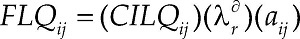
(4)

where λr is an algorithm that takes into account the economic size of the sub-region.

The interpretation of the FLQ is related to the definition of a degree of the provision of regional's supplies (t ij ) with the following relationships:

Thus the regional trade coefficients r ij , are estimated with:

(5)

The estimation of the crossed-holding location coefficient is stated as follows:

(6)

If CILQ ij > 1, then the requirements for input i by the industry j , are obtained inside the region.

If CILQ ij < 1, then the requirements for input by the industry j , are imported.

The regional economic size λ is estimated essentially with regional economic specialization coefficient with respect to the nation's, which is the ratio of regional total output (Et r) to national total output (Et n), and weighted by the factor log2,

which is derived as: where CRESij=EtrEtn.

However, Flegg's methodology was criticized by Brand (1997), who pointed out that the FLQ has a weak theoretical base and poor empirical pedigree. He believes the FLQ offers little to cure the fundamental deficiencies of the genre., and that research funds would be much more effectively employed in any form of survey-based analysis.

The response of the authors, was that the foundation of the FLQ's cross-holding quotients are theoretically appropriate, and that their approach provides a rigorous basis for the testing of the traditional assumption of identical regional and national technology levels.

However, they actually accepted the need to improve the FLQ, in order to give more importance to the different weights of both national and regional economic sizes.

Thus, they developed a reformulation of the FLQ, the RFLQ, Flegg and Webber (1997), which attempted to improve the measurement of the economic size of the region and to avoid the underestimation of regional imports, as well as not allowing the overestimation of the regional multipliers. Hence, the original FLQ was changed, first by improving the estimation of the scalar λ in the original FLQ and second by substituting the crossed holding coefficients, CILQ ij , with the simple location quotient, SLQ i , which is derived as:

(8)

where SLQi=TRETNE; TRE is the total regional employment; TNE is the total national employment, and λ*=log2+TRETNEδ0δ1 and 0 ≤ λ ≤ 1.

However, the interpretation of the RFLQ was similar to the FLQ ij , so they derived the following relationships:

Thus, the regional trade coefficients, r ig , are estimated with:

(9)

Flegg and Webber consider that a value of δ must be near 0.3 in order to minimize the regional differences; this appears to have empirical evidence according to Sánchez Torres (2014) 6.

Despite this improvement, McCann and Dewhurst (1998) raised some concerns about the FLQ formula for the estimation of regional coefficients from national data. They argued there is a need to consider regional specialization when modeling regional economies. As a response, Flegg and Webber (2000) in "Regional size and regional specialization and the FLQ formula", pointed out "(...) empirical work using Scottish data shows that the inclusion of a measure of regional specialization in lq-based formulae does not yield more accurate estimates of regional coefficients. We find too that the FLQ invariably outperforms its main rivals, the SLQ and CILQ".

In an applied research to Finland, Tohmo (2004) validated the conclusions of Flegg and Webber (2000) when comparing the survey-based regional input-output coefficients and production multipliers published by Statistics Finland, to estimates obtained through the application of LQ to national data for the construction of the Keski-Pohjanmaa region. The results led him to support the FLQ quotient as a much better regional input-output coefficient and multiplier than the SLQ and CILQ.

However, contrary to the last argument, Lehtonen and Tykkyläinen (2014) concluded that the core of the problem is the lack of regional information when estimating the simple location quotients. They presented an evaluation of four location quotient regionalization techniques applied in twenty Finnish regions, and addressed the issue of the impacts of the region's properties on the results of the regionalization process. They concluded that the results do not allow for a generalization in any of the four location quotient techniques and would always yield the best results, but they do indicate that the attributes of regions can give information that should be taken into account when selecting the best possible regionalization technique.

Controversially, Kowalewski (2015) in a study applied to Federal Germany, gave empirical evidence on the use of the FLQ formula, pointing out the advantages of the industry-specific FLQ (SFLQ).

Finally, Flegg and Tohmo (2016) re-examined the evidence presented by Lehtonen and Tykkyläinen (2014) about the use of the lqs for the estimation of regional input coefficients and multipliers and stressed out that their evidence is erroneous and that the Flegg's location quotient, yields far superior results, so it should provide a more satisfactory way to generate an initial set of input-output coefficients. The choice of a value for the parameter δ is also examined.

From this review it is clear that the debate has only focused in the advantages and limitations of the main location quotients for the construction of a regional I-O matrix, using only a top-down approach, without any attempt to construct regional matrices using a bottom-up approach, showing their results and making statistical assessments concerning their differences, limitations and advantages.

Methodology for the construction of regional input-output matrices, using a bottom-up approach and its interpretation

The analytical orientation of the construction of regional input-output matrices is based on a theoretical and methodological approach of the economic concentration, which is part of the broader perspective of the spatial dimension of the economy, that we have been developing (Asuad Sanén, 2014, pp. 312-319; Asuad, 2001, pp. 137-158). The main concept of this approach is economic space as well as its derivative economic concepts, territory and region.

Therefore, we assume that economic development and growth tend to be unbalanced, due to the heterogeneity of both natural and economic space; it is not homogeneous or politically bounded to states or municipalities, and given that the spatial distribution of economic activity is highly concentrated in very few areas, economic and population nodes emerge. These are characterized by their economic interactions through production, exchange and consumption. Thus, a node or hub is defined as a site or place, whose economy is characterized by its economic dominance over and connection with a set of minor economic sites that interact and compete with each other, whereas a traditional economic site is defined as a place on the economic space, where economic activities are highly concentrated and from which a set of economic impulses are exerted through economic exchanges; this guides the spatial economic behavior as a whole.

Economic nodes are spatial economic sub-units distributed in a given geographical or political space, with extremely dense economic activity and demographic concentration. Indeed, they behave as the centers of a given market area where most of the spatial concentration of production and consumption are located. Furthermore, they are connected by the economic flows established among them, which as a whole integrate the economic space.

The economic importance of nodes depends on their economic interaction, which is an outcome of the type of connection and market relationships they establish. These can be thought of as economic complementarities or competition among themselves, or just a mixture of both economic interactions. If these interactions were relevant, they would lead to the creation of sub-economic spaces. Therefore, economic space, in order to exist, requires at least the existence of a pair of economic sites or nodes, interacting with each other. Of course, they do not coincide with any geographical or political unit, despite their influence on economic decision-making processes. Only those economies based on market behavior and territorial development define how the economy as a whole is structured in space.

These can be measured with their economic interactions, mainly purchases and sales carried out by companies and consumers. This sectorial-spatial economy and its synergy with the natural and territorial space in a given area, leads to the development of region or sub-regions, integrated by a system of cities and networks of transportation routes, that link them.

In a generic way, the development of regions as spatial economic units is defined as spatial economic functional units , SEFU7, which are an outcome of economic growth and development on space, that is to say, the economic space as a whole. Thus, the development of this spatial unit allows us to know how economic activities have been spatially distributed, defining the spatial structure and behavior of their economy.

According to this theoretical framework, we propose a methodology for the construction of a regional input-output matrix using a bottom-up approach, which has the following steps:

Identification and demarcation of SEFU

The identification and demarcation of the spatial economic functional units of the spatial economic system within a region, requires the specification of the importance and economic specialization within the region as well as its spatialization, by pointing out the particularities of their location. We do this, first, through the identification of nodes and areas of influence, using an index of concentration of economic activity and population, and second, through the establishment of areas of influence, assuming that the pair of nodes which are spatially near are in competition with each other, and taking into account their size and distance with the application of a Reilly index. Actually, as already mentioned, this is the economic space. However, in the first step, we analyzed the economic structure of Sonora, and later we characterized the role and importance of its economic and population nodes as well as their areas of influence. This led us to identify the functional economic spatial units within the region of Sonora. The concentration index is just a result of a ratio between the share of the output of a sub-region (q ir ) in total sub-regional output (q jr ) divided by the same national proportion, which is denoted as:

(10)

where r represents the region or sub-region, and n represents the nation.

The Reilly Index (Asuad, 2016, pp. 362-364), which measures the border between two a pair of nodes that compete with each other, is a function of an inverse relationship between size and distance between them, and is denoted as:

(11)

where BP is the border point; Pa is the population site a ; Pb is the population site b ; Da is the distance to the site a , and Db is the distance to the site b .

Construction of a sub-regional matrix using a bottom-up approach

In order to do this, we used the Mexican economic census to gather regional data from each sub-region at the sub-sector level, or in other words, data coded with three digits according to the Industrial Classification System of North America (NAICS). Then, we estimated the trade coefficients between subsectors at sub-regional level including the sub-regional economic specialization index, which was complemented with a basic accounting framework, in order to apply a set of identities of the regional input-output matrix, at sub-regional level, as the basis for the construction of the sub-regional I-O matrix.

The estimation of the trade coefficients within sub-regions is done with a crossed relative economic specialization quotient (WCLQ) between any pair of economic sectors of the sub-regions, in order to assess the probable economic importance of the transactions of economic sectors given their economic specialization and taking into account their possible economic association as an indirect weight for the calculation of the technical coefficients of production of the economic sectors. This is done just by the transposition of the weighted quotient in a matrix form by economic sector, using in this analysis, the traditional array of rows and columns. In the case of the size of the economic activity, we applied a semi logarithmic quotient in order to measure the relative size of the economic sub-region in terms of the region, which is denoted as:

(12)

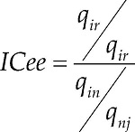
For the analysis of the regional economic specialization of Sonora, we used the quotient of economic specialization (Iee), which is the ratio between the economic specialization of the sub-region in the economic activity i and the same ratio at regional level; this is defined as follows:

(13)

However, this was developed taking into account the average value of the economic activities of the Sonora sub-region compared to the total production of the sub-region. Notwithstanding, the interpretation of the location quotient is the same, thus the coefficient value is equal to or greater than 1.

Thus, the interpretation of the WCLQ ij has to do with the definition of a degree of the provision of sub-regional's s- supplies, t ij , with the following relationships:

Therefore, the sub-regional trade coefficients, r ij , are estimated as the product of the sub-regional provision of supplies, t ij , multiplied by the sub-regional output (P i ) of the subsector, and defined as:

(14)

Hence, in a matrix form, we have the following expressions:

(15)

Basic sub-regional economic accounts

With the economic data from the most recent Mexican economic census, we formulated four basic sub-regional economic accounts, in order to estimate the most important economic transactions of the economic sub-regions of the Sonora region. This is the basis for the construction of the identities from which in turn, we constructed the sub-regional matrices with data from the municipalities (Sonora has 72 municipalities).

i) Sub-regional product account.

It is worth mentioning that the consumption of families and companies (C ) is obtained with the differential between production (P ) and local investment (I ) plus net exports (Xn ).

P = Production, C = Consumption, I = Investment; Xn = Net exports

ii) Sub-regional income and expenditure account.

(18)

(19)

(20)

Thus, regional income, Y , is equal to consumption, C , plus savings (S ); and the total of regional savings, S , results from the difference between production, P , and consumption, C .

Y = Income, S = Savings, G = Expenditure

iii) Sub-regional savings and investment account.

(21)

(22)

This account is based on the assumption that savings, S , are equal to investment, I , so that, when local savings are insufficient to finance investment, the difference will be borrowed from outside of the region.

Ii = Local investment, Ie = External investment

iv) Sub-regional exports and imports account.

(23)

This account is nothing more than the net balance (Bc ) between regional exports (X i ) and imports (M m ) in which regional exports are assumed to be related to national exports and imports to a mixture of purchases outside the region, both national or international.

Bc = Net commercial balance, X i = Regional exports, M m = Regional imports

Therefore, the sub-regional accounts, lead to the establishment of the following accounting identities of the sub-regional input-output matrix.

Total sub-regional supply:

(24)

R s = Regional supply, M = Imports

Total sales:

(25)

V = Sales, Vi = Intermediate sales, Vf = Final sales

Total sub-regional demand:

(26)

Total purchases:

(27)

v) Sub-regional production at factor costs.

(28)

(29)

I = Intermediate cost, VA = Value added, W = wages,

P = profits, t = taxes and subsidies, m = imported inputs

The construction of a multi sub-regional matrix of the economic region of Sonora

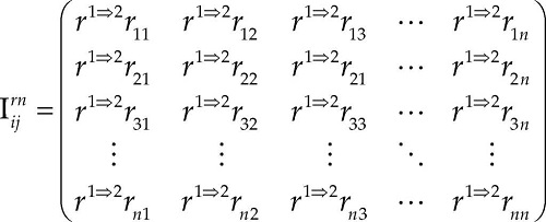
At this stage, purchases and sales between sub-regions are identified through the application of a Moran index of economic interactions, which is validated by the measurement of the spatial dependence between the data of the economic sub-regions. Subsequently, the multi sub-regional matrix was constructed with the use of the technical coefficients of the sub-matrices as a diagonal matrix of the set of the sub-regional matrices of Sonora. Hence, this diagonal matrix integrates estimated purchases and sales of the region, and it is shown above and below the main diagonal of the arrangement of the system of sub-regional matrices. Finally, the RAS method (Appendix 3) was applied in order to obtain the values of the region, applying the traditional way, so purchases were estimated using the total production and purchases through value added.

The construction of the weighted distributions of the sectorial participation in each of the sub-regions, in order to have a measure of the importance of both economic sectors and subsectors in the sub-regions, and use it in order to have a measure of the relative size of the sectors and subsectors in the economy of the sub-regions.

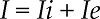
where SEI is the spatial economic interaction; Eijrs is the economic specialization matrix (analysis of spatial interaction), and Iijrs is the spatial correlation matrix (local Moran Index, Paradise, 2016).

This stage has the following steps:

  1. For the construction of the multiple sub-regional matrix (MSE), we started with the sub-regional input-output matrices [15] and converted them into technical coefficients in the main diagonal on [30], or Rijrs.

(31)

  • 2. Find the values of the matrices of sales Vijrs and purchases Cijrs . For this, it is relevant to consider the following:

    • The economic activities are differentiated by their diverse economic distribution among sub-economic regions, so we have an unbalanced economic participation of the economic activities.

    • The economic interaction between a pair of sites can be thought of as spatial dependence if it is established that purchases and sales between two sites are economic flows that are determined by the functional economic interaction of the two sites.

  • 3. Find an economic specializacion indicator eijrs between a pair of sites to identify Cijrs and Vijrs, through the analysis of the spatial interaction (Appendix 2). This looks for a measure that could reflect the distribution and participation of the economic sectors on purchases and sales of both sites.

  • 4. The estimation of the spatial dependence between economic sub-regions and their economic activities, which is done first, through the application of a local Moran Index (I) (Appendix 2), that identifies the spatial correlation between sectors of a pair of sites, based on their physical distance. This coefficient is essential since it allows us to identify purchases and sales between subsectors and between sub-regions, as it is shown in a spatial correlation, which in literature is known as spatial dependence. We assume that this measure accurately reflects the flows of trade of the subsectors of economic activity between sub-regions.

  • 5. The estimation of the economic interactions between economic sub-regions, through purchases and sales of their economic activities, taking into account in their analysis a pair of economic sub-regions. In order to do this, we multiplied matrix I (spatial correlation matrix), with matrix Eijrs(the weighted participation of the economic activities matrix), in order to obtain the SEI of purchases and sales of the economic sub-regions.

  • 6. The estimation of the MSE through the integration of the sub-regional matrices of the region, Rijrs, matrices of purchases, Cijrs, and sales, Vijrs, from SEI, into the traditional matrix arrangement for the multi-regional matrix, which consists of the following:

(32)

  • where mse represents the multiple sub-regional matrix in terms of coefficients of intra-sub-regional and inter-sub-regional trade.

  • 7. Finally, the application of the RAS technique (Appendix 3) to the mse matrix, in order to convert it into the spatial economic interactions matrix, based on the transformation of the spatial economic interactions coefficients into production, commerce and consumption, in monetary terms.

Statistical assessment of both bottom-up and top-down regional matrices of the sonora region

Type of analysis

We did a comparative analysis between both approaches through the identification of chains and economic links. Therefore, two input-output matrices were analyzed: 1) The regional input-output matrix constructed by the Government of Sonora (Bracamontes Sierra and Sánchez G., 2011), using a top-down approach, without sub-regional divisions, and 2) The regional input-output matrix of Sonora constructed with a bottom-up approach, integrated with 10 economic sub-regional units.

In order to evaluate these chains and their linkages we used the traditional approach of sectorial classification of Chenery and Watanabe (1958). For this, we calculated the effects of complete interdependence, through the input-output inverse matrix, which is designated as Z ij .

The traditional classification of Chains, whose effects are above average are classified as follows:

  • Base sectors refer to industrial activities with high forward linkages and low backward linkages.

  • Key sectors refer to economic activities with strong linkages both forward and backward.

  • Sectors of strong drag refer to activities with low forward linkages and high backward linkages.

  • Independent sectors are activities with low linkages, both backward and forward.

Thus, the sectorial classification of the activities was established, taking into account the use of each branch of intermediate inputs according to their average value of production (μ), and the final destination of the average value of intermediate products (ω) of each branch of economic activity. Thus, we have the following indexes:

where Z j is the production of branch j , and Z ij are uses of branch j of inputs of branch i .

where Z j is the production of branch i , and Z ji are uses of branch i of inputs of branch j .

Therefore, according to the relationships between μ and ω we have the following classification:

ωi>ω¯j ωi>ω¯j
μi>μ¯i Base sectors Key sectors
μj>μ¯j Independent sectors Drag sectors

Comparative analysis of backward and forward economic linkages of the economic sectors in both national and regional matrices

The statistical assessment of the regional input-output matrices was done by applying the Watanabe and Chenery approach first to the 2008 national input-output table published by INEGI, and second, to the regional matrices constructed by implementing the bottom-up approach and to the regional matrix constructed by Government of Sonora, using a top-down approach.

Analysis of the economic linkages in each matrix

The results of these economic linkages are analyzed in order to compare them to the observed economic structure of Sonora. In consequence, four tests of hypotheses were applied to see whether the regional matrices constructed using both top-down and bottom-up approaches showed similar averages in their economic sectorial linkages to the national matrix.

We expected that the regional matrix constructed using a top-down approach had a similar economic structure and linkages to the national matrix. However, in the matrix constructed with a bottom-up approach, not only did we expect it to be different to the national matrix, but also to describe the economic structure of Sonora with greater accuracy, because in its construction it takes into consideration the observed elements of the economic structure of the State of Sonora. These assumptions are confirmed in the following 1.

As shown in Table 1, the national matrix has seven key chains and two linkages while the regional matrix constructed using a top-down approach has three key chains, three linkages, and two base chains. Finally, the matrix constructed using a bottom-up approach has four key chains and one base chain.

Table 1 

Sector National Sonora top-down Sonora bottom-up Sonora
BL FL Type BL FL Type BL FL Type Product share %
Primary sector 2.2
_112 0.4 0.4 Ind. 0.2 0.1 Ind. 0.3 0.3 Ind. 1.5
_114 0.1 0.1 Ind. 0.0 0.0 Ind. 0.1 0.1 Ind. 0.7
_115 0.0 0.0 Ind. 0.1 0.0 Ind. 0.0 0.0 Ind. 0.0
Secondary sector 64.7
_2 3.0 3.5 Key 0.7 5.1 Pull 3.5 2.2 Key 25.9
_311 1.8 3.4 Key 1.5 3.8 Key 0.6 0.7 Ind. 6.0
_312 0.3 0.5 Ind. 0.7 0.8 Ind. 0.7 0.6 Ind. 3.1
_327 0.7 0.3 Ind. 0.1 0.2 Ind. 1.9 2.2 Key 2.2
_331 1.5 0.7 Pull 0.7 0.3 Ind. 0.5 0.5 Ind. 6.6
_332 0.9 0.4 Ind. 0.5 0.2 Ind. 0.6 0.7 Ind. 2.7
_334 1.8 1.4 Key 1.8 0.8 Pull 4.7 5.9 Key 3.1
_336 1.1 1.6 Key 6.3 0.5 Pull 0.2 0.1 Ind. 13.2
_339 0.5 0.4 Ind. 0.8 0.3 Ind. 1.0 0.9 Pull 1.9
Tertiary sector 33.0
_43-46 3.3 1.0 Key 2.6 1.6 Key 1.1 1.0 Key 15.0
_48_49 1.2 1.3 Key 1.0 0.7 Pull 0.5 0.6 Ind. 1.9
_51 1.2 0.5 Pull 0.4 0.9 Ind. 0.7 0.9 Ind. 3.6
_52 1.3 1.1 Key 0.6 0.5 Ind. 0.0 0.0 Ind. 0.3
_53_56 0.0 0.8 In. 1.4 1.6 Key 0.7 0.8 Ind. 4.9
_6 0.0 0.6 Ind. 0.1 1.3 Pull 0.3 0.3 Ind. 2.3
_7 0.4 0.7 Ind. 0.2 0.8 Ind. 0.6 0.8 Ind. 3.3
_8 0.5 0.2 Ind. 0.2 0.3 Ind. 0.3 0.3 Ind. 1.7

Note: BL = backward linkages; FL = foward linkages.

Source: own elaborations base don data from the 2008 national input-output the 2008 matrix of Sonora and the Censos Económicos 2009 of the INEGI. See Apendix 5 for the code of the economic sectors.

However, if we look at the following graphics we see clearer similarities between the information generated from the matrix constructed using a top-down approach with the national matrix, and differences between the latter and the one constructed using a bottom-up approach.

Graph 1 Sectoral linkages in the national input-output table. 

The key sectors for both the regional and national matrices are Food industry (311) Wholesale trade and retail (43-46), Professionals in Real Estate services, Corporate and Business Support and Waste management and Waste.

Graph 2 Sectoral linkages in the regional input-output table constructed using a top-down approach. 

While the comparison of the graph of sectoral linkages with information from the national grid and built from below, it is observed that in key sectors have in common only two on Mining (2), Wholesale trade and retail (43-46). This comparison is true but given the importance of mineral at the regional level, as well as services in general.

Graph 3 Sectoral linkages in the regional input-output table, built from bottom to top. 

However, this analysis is not rigorous enough to find out the statistical differences between the regional matrices with the national one, thus we apply the two -tailed test hypothesis, in order to look for them.

Statistical assessment of the two-tailed test hypothesis

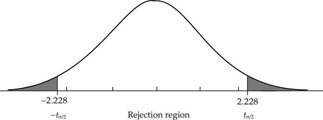
This test is also known as non-directional hypothesis , and it is a standard test of statistical significance, which means that the differences in the results do not occur randomly. Succinctly, two-tailed tests divides the 0.05 probability value (p) into two and puts each half on each side of the bell curve in order to determine if there is a relationship between variables in one of the directions (See Appendix 4). So, it does not predict whether the parameter of interest is greater or less than the reference value specified in the null hypothesis. Hence, with this statistical assessment of the regional matrices constructed using both bottom-up and top-down approaches we wanted to determine if their economic linkages are on average different or similar than the national matrix, in order to identify if the regional matrices were similar to the nation, assuming that if this is the case there would be no difference between the region and the nation. Therefore, we concluded that is just a change of scale from regional level to national, and inadequate for economic regional modeling or regional policy and planning.

According to the results of the two-tailed test hypothesis analysis, we have the following results:

Test I. Backward linkages:

  • 1.The average backward linkages observed in the state matrix constructed using a top-down approach are very similar to the backward linkages of the national matrix.

  • 2.The backward linkages observed in the matrix constructed using a bottom-up approach are on average, different than the observed linkages in the national matrix.

Test II. Forward linkages:

  • 3.The forward linkages observed in the state matrix constructed using a top-down approach are very similar to the forward linkages observed in the national matrix.

  • 4.The forward linkages observed in the matrix constructed using a bottom-up approach are on average, different that the observed linkages in the national matrix.

Test III. No linkages:

  • 5.The independent sectors observed in the state matrix constructed using a top-down approach are very similar to the independent sectors in the national matrix.

  • 6.The independent sectors observed in the matrix constructed using a bottom-up approach are different on average to the observed sectors in the national matrix.

Test IV. Forward and backward linkages

  • 7.The key sectors reported by both the matrices are on average different to those observed in the national matrix.

Concluding remarks

It is observed that there are important differences between both regional matrices. The top-down regional matrix is more similar to the national matrix in terms of economic linkages. Furthermore, significant differences arise from the regional matrices, in terms of the backward linkages and independent sectors, which is closer to the national case (top-down matrix). Therefore, we conclude that this article shows empirical evidence to support the need for the construction of regional input-output matrices constructed using a bottom-up approach. This is already in a methodological proposal we made, despite the need for more simplification and operationalization procedures for its application. We think this shows a more accurate perspective of regional structures than the top-down matrices.

Although this article is an outcome of a set of methodological experiences that are still in process of review and discussion, we believe we present solid elements to support our bottom-up theoretical and methodological approaches; we also believe there is still a need to use this topic as a new line of research for the construction of regional input-output matrices.

According to our view, the main theoretical and methodological challenge, which was already achieved, is the construction of regional input-output matrices at intra-regional level, given that in the literature, the construction of inter-regional matrices has important theoretical and technical proposals and that it also has enough empirical evidence related to their application at national and international levels (See Miller and Blair, 2009; Sargento, 2009; Lahr, 2001).

Finally, it is important to stress out that this work is part of a line of research developed over a long period of time and still continues in CEDRUS, applying in to the construction and analysis of the regional input-output matrices with the use of a bottom-up approach. This already has opened up new research proposals for applied studies, the development of spatial economic analyses and experimental researches of regional and urban economic studies.

References

Armenta A. Modelo insumo-producto para Tabasco (Integración de la Matriz de Insumo Producto). Villahermosa, Tabasco: Universidad Juárez Autónoma de Tabasco. Collection "José Ma. Pino Suárez. Estudios Regionales y Desarrollo"; 2007. [ Links ]

Aroche F. La investigación sobre el modelo de insumo-producto en México. Orígenes y tendencias. Estudios Económicos. 2013; 28(2):249-64 [ Links ]

Asuad Sanén N.E. Economía regional y urbana. Introducción a las teorías, técnicas y metodologías básicas. Puebla: Benemérita Universidad Autónoma de Puebla, Colegio de Puebla, and Asociación de Ex Alumnos de la FE-UNAM; 2001. [ Links ]

Asuad Sanén N.E. Pensamiento económico y espacio. Mexico, Mexico City: Graduate School of Economics, UNAM. First Volume, Collection "Economía Regional y Urbana"; 2014. [ Links ]

Asuad Sanén N.E. Desarrollo regional y urbano. Tópicos selectos. Mexico: Facultad de Economía, UNAM; 2016. [ Links ]

Asuad Sanén N.E, Quintana Romero L, Ramírez Hernández R. Una propuesta metodológica para la delimitación de regiones económicas a través de un índice de interacciones económicas. El caso de la región económica noreste del país. Problemática regional en México: hacia una agenda para el desarrollo. Mexico: Asociación Mexicana de Ciencias para el Desarrollo Regional, A.C. (amecider); 2008. [ Links ]

Asuad N.E, Sánchez Gamboa J.M, Garduño K. A comparative analysis for constructing regional input-output tables, for Sonora, Mexico, from the bottom-up approach, its methodology and advantages over the top-down approach. 23rd International Input-Output Conference & 5th Edition of the International School of I-O Analysis. Mexico: Mexico City; 2015 22-26 June. [ Links ]

Asuad N, Vázquez C, Quiñones Luna E. Manufacturing clusters in functional economic North-Central region of Mexico: A spatial approach using input-output analysis. 23rd International Input-Output Conference & 5th Edition of the International School of I-O Analysis. Mexico: Mexico City; 2015 22-26 June. [ Links ]

Bracamontes Sierra Á, Sánchez G. J.M. Matriz Insumo Producto para el Estado de Sonora, 2011: actualización y regionalización estadística. Hermosillo, Sonora: Gobierno del Estado de Sonora, Secretaría de Economía, and Consejo para la Promoción Económica de Sonora; 2011. [ Links ]

Brand S. On the appropriate use of location quotients in generating regional input-output tables: A comment. Regional Studies. 1997; 31(8):791-4 [ Links ]

Brand S. A note on methods of estimating regional input-output tables: Can the FLQ improve the RAS algorithm?. Available through: The Busines School whith Plymouth University; 2012. [Working Paper] <https://www1.plymouth.ac.uk> [ Links ]

Callicó López J, González E, Sánchez L. La matriz interregional del Centro Occidente de México. In: Callicó, J. et al. Insumo producto regional y otras aplicaciones. Mexico: Universidad Autónoma Metropolitana-Azcapotzalco, UNAM, and Universidad de Guadalajara; 2003. 165-9 [ Links ]

Chapa Cantú J, Ayala E, Hernández D. Modelo de insumo producto para el noreste de México. Ciencia UANL. 2009; 12(4):409-16 [ Links ]

Chenery H, Watanabe T. An international comparison of the structure of production. Econometrica. 1958; 26(4):487-521 [ Links ]

Dávila F. Matriz de insumo-producto de la economía de Coahuila e identificación de los flujos intersectoriales más importantes. Economía Mexicana. Nueva Época. 2002; XI(1):79-162 [ Links ]

Dávila, F. (coord.) (2015). Modelos interregionales de insumo producto de la economía mexicana. México, México City: Miguel Ángel Porrúa, Universidad Autónoma de Coahuila, and Universidad Autónoma de Nuevo León. [ Links ]

Devore J.L. Probability and Statistics for Engineering and Sciences. Belmont, CA: Duxbury Press; 1990. [ Links ]

Flegg A.T, Webber C.D. On the appropriate use of location quotients in generating regional inputoutput tables: Reply. Regional Studies. 1997; 31(8):795-805 [ Links ]

Flegg A.T, Webber C.D. Regional size, regional specialization and the FLQ formula. Regional Studies. 2000; 34(6):563-9 [ Links ]

Flegg A.T, Tohmo T. Estimating regional input coefficients and multipliers: the use of flq is not a gamble. Regional Studies. 2016; 50(2):310-25 [ Links ]

Flegg A.T, Webber C.D, Elliot M.V. On the appropriate use of location quotients in generating regional input-output tables. Regional Studies. 1995; 29(6):547-61 [ Links ]

Fuentes N.A. Matrices de insumo-producto de los estados fronterizos del norte de México. México: Universidad Autónoma del Estado de Baja California; 2003. [ Links ]

Fuentes N.A. Construcción de una matriz regional de insumo-producto. Problemas del desarrollo, Revista Latinoamericana de Economía. 2005; 36(140):89-112 [ Links ]

Fuentes N.A, Brugués A. Modelos de insumo-producto regionales y procedimientos de Regionalización. Comercio Exterior. 2001; 51(3):33-54 [ Links ]

Garduño K, Sánchez J.M, Asuad N.E. Airport cluster in Mexico City, a spatial approach using a regionalized input-output matrix from top-down approach. 23rd International Input-Output Conference & 5th Edition of the International School of I-O Analysis. Mexico: Mexico City; 2015 22-26 June. [ Links ]

Garduño K, Sánchez J.M, Asuad Sanen N. Exploratory analysis of the use of a multiregional input-output matrix for the analysis of the main urban impacts of the new México City Airport. 24th International Input-Output Conference & 6th Edition of the International School of I-O Analysis. Seoul: Korea; 2016 4-8 July. [ Links ]

Kowalewski J. Regionalization of national input-output tables: empirical evidence on the use of the flq formula. Regional Studies. 2015; 49(2):240-50 [ Links ]

Lahr M.L. A review of literature supporting the hybrid approach to constructing regional input-output models. Economic Systems Research. 1993; 5(3):277-93 [ Links ]

Lahr M.L. A strategy for producing hybrid regional input-output tables. In: M.I. Lahr and E. Dietzenbacher (eds.) Input-Output Analysis: Frontiers and Extensions. London: Palgrave; 2001. 1-31 [ Links ]

Lahr M, Stevens B.H. A study of the role of regionalization in the generation of aggregation error in regional input-output models. Journal of Regional Science. 2002; 42(3):477-507 [ Links ]

Lehtonen O, Tykkyläinen M. Estimating regional input coefficients and multipliers: is the choice of a non-survey technique a gamble?. Regional Studies. 2014; 48(2):382-99 [ Links ]

Maya M, Sánchez J.M, Asuad N.E. Regional vertical specialization of the automotive chain in the Central North region of México and its main effects on regional production structure: A spatial approach using an input-output regional table. 23rd International Input-Output Conference & 6th Edition of the International School of I-O Analysis. Mexico: Mexico City; 2015 22-26 June. [ Links ]

Maya M.N, F A. Sánchez, Asuad Sanen N. Spatial analysis of regional input-output of the automotive supply chain and its impact on economic development in the economic functional region Northeast Mexico. 24th International Input-Output Conference & 6th Edition of the International School of I-O Analysis. Seoul: Korea; 2016 4-8 July. [ Links ]

McCann P, Dewhurst J.H.L.L. Regional Size Industrial location and input-output expenditure coefficients. Regional Studies. 1998; 32(5):435-44 [ Links ]

McDonald J.F. Fundamentals of Urban Economics. USA: Prentice Hall; 1997. [ Links ]

Miller R.E, Blair P.D. Input-Output Analysis: Fundations and Extensions. Cambridge: Cambridge University Press; 2009. [ Links ]

OECD (Organisation for Economic Co-operation and Development)Redefining Territories. The Functional Regions. Paris: OECD Publications; 2002. [ Links ]

OECD (2013). Defining regions and functional urban areas. In: OECD Regions at a Glance 2013. [Online] OECD Publishing. Available at: <http://dx.doi.org/10.1787/reg_glance-2013-47>. [ Links ]

Paradise, M. (2016). Moran's autocorrelation coefficient in comparative methods. [pdf] Available at: <https://cran.r-project.org/web/packages/ape/vignettes/MoranI.pdf>. [ Links ]

Sánchez Torres, D. (2014). Construcción y uso de matrices regionales insumo- producto en México. In: L. Quintana and A. Roldán (cords.). Técnicas modernas de análisis regional. Serie Análisis Regional (pp. 119-158). Mexico: Facultad de Estudios Superiores Acatlán and Valdés Editores. [ Links ]

Sargento, Marto A.L. Regional Input-Output Tables and Models. Doctoral thesis Faculty of Economics, University of Coimbra; 2009. [ Links ]

Stone, R. (ed.) A Programme for Growth 3, Input-Output Relationships, 1954-1966. Chapman and Hall, London: Cambridge University, Department of Applied Economics; 1963. [ Links ]

Tohmo T. New developments in the use of location quotients to estimate regional input-output coefficients and multipliers. Regional Studies. 2004; 38(1):43-54 [ Links ]

Vázquez C, Asuad N.E, Zafra K. Economic interactions productive chains and formation of manufacturing clusters in the functional economic North Central region of México: a case of regional input-output from the bottom-up approach. 24th International Input-Output Conference & 6th Edition of the International School of I-O Analysis. Seoul: Korea; 2016 4-8 July. [ Links ]

West G.R. Regional trade estimation: A hybrid approach. International Regional Science Review. 1990; 13(1-2):103-18 [ Links ]

*This essay is part of the Project PAPIIT IN307114 "Clusters, cadenas productivas e identificación del potencial de integración productiva y del aprovechamiento de las ventajas competitivas de las regiones económicas de México" ["Clusters, Productive Chains and Identifying the Potential for Production Integration and Leveraging of the Competitive Advantages of the Economic Regions of Mexico"] supported by the Dirección General de Asuntos del Personal Académico at the Universidad Nacional Autónoma de México (DGAPA-UNAM). This article comes after a previous one which presented the first phase for the implementation of the methodology: Normand Eduardo Asuad Sanén and José Manuel Sánchez Gambóa (2016). An exploratory and comparative analysis for the construction of regional input-output matrices between bottom-up and top-down approaches, in process of editorial review. We also want to express our recognition to students and Centro de Estudios de Desarrollo Regional y Urbano Sustentable (CEDRUS) member professors for their collaboration; without them, the creation of this article would not have been possible, particularly to Karina Garduño Maya, Krista Zafra García, Cristina Vázquez Ruiz, Marcos Maya Luis Alberto Flores, Alejandra Ibañez Tercero, Sergio Rodríguez, Francisco Alfredo García, and Adrian García. Furthermore, I am also very grateful to Dra. María Dolores Sánchez for its statistical comments and to Dr. William Sughrua and to William Ismael Sughrua Martínez for the English revision.

1Presented in the 23th International Input-Output Conference in Mexico City, 2015: 1) Asuad, Vázquez, and Quiñones Luna (2015); 2) Asuad, Sánchez Gamboa, and Garduño (2015); 3) Maya, Sánchez, and Asuad (2015), and 4) Garduño, Sánchez, and Asuad (2015).

2Presented in the 24th International Input-Output Conference in Seoul, Korea, 2016: 1) Garduño, Sánchez, and Asuad (2016); 2) Vázquez, Asuad, and Zafra (2016), and 3) Maya, Sánchez, and Asuad Sanén (2016).

3Own elaboration with data published by the Instituto Nacional de Estadística y Geografía (INEGI), available at: <www.inegi.gov.mx>. See gross domestic product by economic sector of economic activity 2008-2012, the Anuario Estadístico y Geografía de Sonora 2014 , and México en cifras 2008 .

4It is worth mentioning that despite the comparison we made between the outcomes of both matrices using the entire political unity of the state of Sonora México, an absolute requirement for the comparison between both approaches, we believe this does not have any effect in how the regional I-O matrix was constructed, given that it originated from the spatial economic functional units (SEFU) of Sonora, which as a whole integrate the political unity of Sonora.

5This part was developed based on Brand (1997).

6According to Sánchez Torres (2014, p. 135), Bonfilgio (2009) calculated a value of delta in 0.36 in 1 000 national matrices and 20 000 sub-regional matrixes, with a Monte Carlo's simulation statistical analysis.

7In the regional and urban literature, there is a consensus on the concept of functional regions, which are defined as spatial units that result from the organization of economic and social relationships in space. Furthermore, theoretically, this concept has been treated through different perspectives: theory of location, theory of market areas, theories of poles of economic growth along with their respective debates in explaining urban territories, especially from Christaller (1933) and Losch (1944) as well as in current urban policy issues (e.g. , OECD, 2002 and 2013). According to our conception, the essential aspect of functional economic regions is the identification of economic activities in space through its location and economic sectorial characteristics, as well as the role and interactions they establish, which give rise to a economic structure on space, and leads to the creation and development of an economic spatial unity (See Asuad Sanén, 2014, pp. 339-356). For the specific economic functions in a city, see McDonald (1997). However, there are different techniques for the identification and measurement of the economic spatial functional region: gravity models, labor market models and commercial interactions areas. Nevertheless, we have developed a methodology for the identification and analysis of these units and their economic interactions through the identification of the sub-regional productive chains, whose details are presented in appendices 1 and 2.

8The multiplication is done element by element, so that each element had a corresponding weight according to weight calculated for the pair of corresponding sites. In other words, γ ij = (ABS )(x ij * ij ) (Asuad Sanén, Quintana Romero, and Ramirez Hernández, 2008).

9This section is based on Brand's consideration (2012) of the RAS method as an estimator of regional trade.

10 Devore (1990) proposes seven steps for the realization of hypothesis testing: 1) identify the parameter of interest and describe it in the context of the problem; 2) determine the null value and set the null hypothesis; 3) set the appropriate alternative hypothesis; 4) Introduce the formula to obtain the values of the test statistic; 5) set the rejection region for statistical significance level α; 6) calculate the sample quantities, replace them in the formula and calculate the statistical value, and 7) decide if H0 is rejected and set conclusions in the context of the problem. Steps 2 and 3 must be performed before examining the data.

APPENDIX 1

The economic specialization indicator, eijrs, between a pair of sites

This weight matrix is obtained, first by calculating the shares of each site in each economic activity, that is, the percentage involved in each of the activities, thus, we obtain as many entries as the number of sites calculated. Then, a score for each of the site's participations is obtained by adding the units per site. As a next step, a new entry per site is calculated from the scores, so that each share represents an overall weight (which includes the effect of all previous economic activities) per site (Asuad Sanén, Quintana Romero, and Ramirez Hernández, 2008). Finally, the cross weighting matrix, which results from of multiplying the score or score participation of site i by the participation of the score of generates a weight or cross weighting matrix j , i.e. the weight involving sites i , j . So this weight or cross weighting ranks i , j of the new array of crosses weights.

This correlation matrix is multiplied by the cross weight matrix8, this operation high interactions resulting from high real interaction sites, such as is reflected, while the high correlations, but result of two sites similarly low values reflect low and would not high as with simple correlation coefficients (Asuad Sanén, Quintana Romero, and Ramirez Hernández, 2008).

The probabilistic index of economic interactions between sites was determined by obtaining the statistical association between a pair of sites. In other words, it was calculated using the statistical correlation coefficient for a series of subsequently calculated weights cross type, and thus transforming the correlation coefficient interaction index; it is represented in the following:

S is the vector of economic sites, S = (s 1 , s 2 , ..., s n ) in which n as their amount in a given economic region. A = (a kl ) matrix of economic activities with k = 1,..., m sectors of economic activity and with l = 1, ..., n + 1, m > n for all k .

R = (r ij ), and is a matrix of size n ×n .

We define R as the partial correlation matrix between different sites s j , in which the calculation of partial correlation coefficients of Pearson (r ij ) is performed through the activity of matrix A activity as follows:

α and β are estimated with Ordinary Least Squares (OLS) coefficients. According to the definition of the partial correlation of Pearson, if the relation r ij = r ji is true, then R would be a symmetric matrix:

It is clear that r ij = 1, for all i .

Now let A′= (a kl ) matrix 'scores' or arising from A, containing such shares for each site in each a kl s j activity that is:

Then:

for all l , a m +1l Sea now a ' m +1l = pond l this is defined as the total weight for each site s j .

Then have P = (p ij ) is an n ×n matrix, called the P matrix cross weights and is defined as follows:

P ij = pond i * pond j for all i and for all j

That is, 'cross' total weights sites if and s j resulting cross weighting p ij . Clearly p ji = p ij = P is a symmetric matrix.

So there has to be economic interaction between a pair of sites i , j for all i , j given by the economic relation between the different s j .

It now has:

That is to say:

Therefore, it is through multiplication element by element of R and P defined e ij . Finally, let E be a matrix of n ×n matrix called economic interactions, defined below:

where

So eij* [0,1], it is called index economic interaction between the two sites i , j .

Here it is worth noting that E is also a symmetric matrix.

APPENDIX 2.

The local Moran Index

The local Moran Index is a measure of spatial correlation between the economic activities i of each sub-region in r n which are linked as pair of subsectors ij and sub-regions, r n . The concept of bivariate spatial correlation refers to the degree of similarity between the systematic value of the variable i observed at a certain location and values of another variable observed in "neighboring j " locations. This coefficient is equivalent to a coefficient of correlation between two variables in the same locations as it associates the value of the variable in neighboring or contiguous locations. This coefficient is used to measure spatial dependence between sectors of different regions or sites. This statistic considers the variables as deviations or analysis of covariance (Moreno and Vayá, 2000, p. 37).

Thus, in a matrix from we have a spatial correlation matrix, which is specifying as follows:

The index is denoted as:

where

x is the variable of analysis; is the mean; i is the productive sector i ; j is the productive sector j , and Wrn is the weight matrix between n regions or sites.

APPENDIX 3.

The RAS method9

The scaling algorithm of a bi-proportional matrix-scaling algorithm known as RAS, and proposed by Stone (1963). Is used its application as a methodology for the estimation of regional trade and is outlined as follows. We use the mse matrix to create a matrix T to show purchases of the sub-regional sectors in the regional market:

(i)

where x^ is a vector of regional sectors, in which ^ denotes a diagonalized vector, and T contains t ij elements t ij , an i dimensional intermediate column vector with elements:

(ii)

and a j dimensional intermediate row vector with elements:

(iii)

It defines the total value of sub-regional purchases from the regional market with t as given (for example ∑ i t ij ). The application of the RAS algorithm to regions, seeks to estimate R, the unknown transactions between sub-regional sectors (r ij elements), knowing only the observed intermediate row and column vectors of R, (elements r i and r j ), which are structured just like t i and t j in T. The total value of the transactions r of intra-sub-regional sectors, r is therefore known as r = ∑ i r i .

1. Column vector z is formed with elements r i /t i . For example, the propensities to purchase each sector's output from the sub-regional rather than regional market, and this is applied to T as a multiplicative scalar across its rows:

(iv)

The intermediate column vector R0 * now has elements, r0i *=ri.

2. A row vector s is formed with elements rj/r0i * from the intermediate row vector of R0 *; the columns R0 * are then scaled to correspond with r j as:

The first (iv) and second (v) steps of the algorithm are then repeated, with z being created with elements ri/r2j * and applied to R1 * to create R2 *; s is then

formed with r j and r2j * , etc. This process is iterated until both z and s approach the unit vectors, with the resulting matrix Rn * being the final estimate of R3.

APPENDIX 4.

The two-tailed test hypothesis

The non -directional hypothesis testing seeks to determine each difference parameters of the chains of regional matrices regarding national development-. In order to decide which of two contradictory claims about the parameters is correct, we use the hypothesis test confidence interval for a population mean with known σ (Devore, 1990). The simplicity of this type of evidence and its applicability in this research allows us to obtain certainty and clarity. At first, it considered the null hypothesis that μ has a particular numeric value, the null value μ0, μ- represents the range of the sample size n , μ-r is the sample mean:

μx-= μ with standard deviation σx-=σ/n so that when H0,μx-=μ0 holds true.

Such tests are considered non-directional or with two tails because of their corresponding rejection region illustrated in the probability distribution curve presented below.

A non-directional alternative hypothesis, does not predict whether the parameter of interest is greater or less than the reference value specified in the null hypothesis. In other words, with the regional bottom-up matrices we wanted to determine if their economic linkages are on average different or similar to the national matrix10.

Development of the statistical tests

Test I: backward linkages (BL)

H0: The average backward linked sectors in regional arrays are equal to the average of backward linked sectors in the national matrix.

H1: The average backward linked sectors in regional matrices are different to the average of backward linked sectors in the national matrix.

Test II: of forward linkages (FL)

H0: the average of the sectors with forward linkages in regional arrays are equal to the average of the sectors with forward linkages in the national matrix.

H1: the average sectors with forward linkages in regional matrices are different to average of the sectors with forward linkages in the national matrix.

Test III: absence of linkages (I)

H0: the average of the independent sectors in regional matrices are equal to the average of independent sectors in the national matrix.

H1: the average of the independent sectors in regional matrices are different to the average of independent sectors in the national matrix.

Test IV: of forward and backward linkages (K)

H0: the average of the key sectors in regional matrices is equal to the average of key sectors in the national matrix.

H1: the average of the key sectors in regional matrices are different from the average of key sectors in the national matrix.

Assuming the average of linkages is distributed as a normal distribution (μ0 = 0.5). The student's t statistic is used with 0.05 degrees of freedom.

where μ it is the sample mean of the data; n it is the sample size, and σ is the standard deviation.

Critical value: -tα/2'n-1,tα/2'n-1; Rejection area: t'-tα/e'n-1,ttα/e'n-1α= constant and n -1.

Table A4.1 Parameters of the chains of both regional and national matrices using both approaches. 

Linkages type National matrix Regional Sonora top-down Regional Sonora bottom-up
μ σ μ σ τ μ σ τ
Backward linkages I 0.500 7.071 0.40 8.49 -0.22 0.30 9.90 -0.38
Fordward linkages II 0.350 9.192 0.30 9.90 -0.09 0.20 11.31 -0.25
No linkages III 0.500 7.071 0.45 0.45 -0.12 0.70 4.24 0.89
Forward and backward linkages IV 0.350 9.192 0.15 0.15 -0.31 0.20 11.31 0.25

Table A4.2 Hypothesis tests for both national and regional input-output matrices input-output matrices using both approaches. 

Test H 0 H 1 Critical value 0.465 Regional Sonora top-down Regional Sonora bottom-up
I H0; u r ≅ 0.5 H1; u r ≠ 0.5 P (t n-1 = 0.5) = -0.22 Accept H0 -0.38 Reject H0
II H0; u r ≅ 0.35 H1; u r ≠ 0.35 P (t r−1 = 0.35 = −0.09 Accept H0 -0.25 Reject H0
III H0; u r ≅ 0.5 H1; u r ≠ 0.5 P (t r−1 = 0.5 = −0.12 Accept H0 0.89 Reject H0
IV H0; u r ≅ 0.35 H1; u r ≠ 0.5 P (t r−1 = 0.5 = −0.31 Accept H0 0.25 Reject H0

APPENDIX 5

Number Sectors
112 Animal breeding and their production
114 Fishing and hunting
115 Services related to agricultural and forestry activities
2 Basic industry
311 Food industry
312 Beverage and tobacco industries
327 Nonmetallic mineral products manufacturing
331 Basic metal industry
332 Metal products manufacturing
334 Computers and other electronic equipment
336 Manufacturing of transportation equipment
339 Other manufacturing industries
43-46 Wholesale and retail activities
48-49 Transportation, postal services and warehousing
51 Mass media information
52 Financial and insure services
53-56 Urban services
6 Social services
7 Cultural and recreational services
8 Other services

Received: August 09, 2016; Accepted: September 28, 2016

Autor para correspondencia. nasuad@yahoo.com


Discusión

Review of "A methodological proposal for the construction of a regional input-output matrix using a bottom-up approach and its statistical assessment", by Normand E. Asuad Sanén and José M. Sánchez Gamboa

Michael L. Lahra 

a Research Professor at the Rutgers Economic Advisory Service (R/ECON(tm)), Edward J. Bloustein School of Planning & Public Policy, Rutgers, The State University of New Jersey (United States of America). Correspondence: lahr@rugers.edu.

Methods used to construct regional input-output accounts are important and are becoming ever more interesting. They are becoming more important partly because information used to build such accounts is becoming ever rarer. Regardless, I like studies that investigate such matters as they have been an interest of mine since I started my career in regional economics.

Key issues in such matters are the sectoral and geographic detail used to build such accounts. It is hard to get too much sectoral detail. But there is a fine line between too much and too little geographic detail, mostly because of the lack of available data on interregional commuting and trade. In this regard the current study's use of functional economic areas (the SEFUs in the paper) seems to get at the "right stuff," especially if they somehow can be readily split and combined to form politically important regions like states to enable the resulting models to address issues of regional political concern in Mexico.

Still, there are some issues with the paper with which I disagree. In particular, I am not keen on FLQs and related short-cut measures that are applied to a technology matrix to form regional direct requirements matrices. These measures do not sufficiently address account for the locational and economic geographic features of the various regions or industries that are investigated. I suggest instead that the authors apply a more general econometrically derived set of regional purchase coefficients (RPCs) in Treyz and Stevens (1985) and Stevens, Treyz, and Lahr (1989). Miller and Blair (2009) refer to these RPCs as "regional supply percentages." Flegg-based measures like the WCLQs used in the paper are far less specific in the way they rows-only adjustment national technology (with international trade already accounted) for interregional trade.

Such econometrically derived RPCs can be estimated for goods-producing industries from a reasonably large sample of freight transportation flows that include a fair amount of sectoral detail, the origins of goods production, and approximate destinations of goods delivery. The appendix Stevens, Treyz, and Lahr (1989) suggests a functional form (an odd one but it keeps the value of the estimate between 0 and 1) and a selection of variables used in conjunction with data in U.S. commodity flow data from 1977. (It may be that a better functional form can be derived.) So does Treyz and Stevens (1985). Note that they use a sort of location quotient for the good (actually the supply/demand ratio for the commodity in the region), the region's demand for the commodity, the commodity's value/weight ratio, the region's share of the nation's land area, the region's relative establishment size within the region, some industry identifiers, and other locational determinants. Of course, the RPCs for services remain estimated best by some sort of truncated location quotient based on labor income. Exceptions are producer services and hotels, which undoubtedly need some special treatment. The same goes for construction, which by definition occurs at the building location, although labor can come from quite a distance for special projects.

There are other matters that I find surprising or that are not given enough detail in the discussion. For example, it seems that Mexico not have a consumer expenditure survey, which I find improbable. If such survey data are available, the authors could gain some insight into spending differentials of households by state if not by SEFU? The same goes for the spending of state and local governments, which typically make budget information publicly available in democratic societies. I am quite surprised that, for each state, both public and private investment data are available by industry from which the investments are purchased. These data, which are shown in equation [19], are something we generally lack here in the U.S. even at the national level. And when they are available, they are estimates and part of the dual purpose (along with estimating detail in the property-type income in the GDP by income accounts) of benchmarking national accounts. The sources for each piece of data, which are apparently available according to equations on pages 20, 21, and 22, should be cited.

The notation is lacking a bit starting on page 23. I don't get how you derive the Cs and Vs or, for that matter, even how they might be derived from what you have given us so far. I suspect these matrices of interregional trade would have to be through some doubly constrained gravity model.

I think it might be interesting to contrast the approach you suggest here to the top-down approach developed in the attached Haddad (2014) paper, which is quite simple, next I will try to review this other piece to see if it can be used to econometrically develop regional purchase coefficients for the states of Mexico.

References

Haddad E.A. Trade and interdependence in Lebanon: An Interregional input-output perspective. Journal of Development and Economic Policies. 2014; 16:5-45 [ Links ]

Stevens B.H, Treyz G.I, Lahr M.L. On the comparative accuracy of RPC estimating techniques. In: R.E. Miller, K.R. Polenske, and A.Z. Rose (eds.). Frontiers in Input-Output Analysis. New York: Oxford University Press; 1989. 245-57 [ Links ]

Treyz G.I, Stevens B.H. The TFS regional modelling methodology. Regional Studies. 1985; 19(6):547-62 [ Links ]


Discusión

Comentario al artículo "A methodological proposal for the construction of a regional input-output matrix using a bottom-up approach and its statistical assessment" de Normand E. Asuad Sanén y José M. Sánchez Gamboa

Pablo Ruiz Nápolesa 

a Profesor de la Facultad de Economía, UNAM (México). Correspondencia: ruizna@unam.mx.

Este artículo trata de la presentación formal de una técnica de análisis regional en el ámbito del insumo-producto, que resulta novedosa respecto a lo que tradicionalmente se ha hecho hasta ahora en el insumo-producto. La técnica consiste en la construcción de un modelo regional de insumo-producto de abajo hacia arriba o botton-up, de la que hay pocos antecedentes, ya que los modelos más utilizados son los llamados de arriba hacia abajo o top-down. El tema se refiere al origen de la información inicial, en el caso de los modelos top-down se parte de la matriz de insumo-producto nacional, la cual se ajusta con datos locales para obtener una matriz de insumo-producto local o regional.

El estudio comienza con una revisión amplia de la bibliografía respecto al análisis regional de insumo-producto a nivel internacional, incorporando la evolución de la temática en estudios relativamente más recientes. En este recorrido destaca, en especial, la polémica respecto a cómo introducir la noción de espacio económico como concepto de región, a diferencia de concebir ésta como territorio político y administrativamente delimitado, es decir un estado o municipio. En consecuencia, surge un problema relacionado con la medición de transacciones económicas que implica esta noción particular de región.

No obstante, lo que tiende a prevalecer a lo largo del tiempo es el modelo de arriba hacia abajo, esto es, la consideración de las relaciones intersectoriales a nivel nacional que se van ajustando para construir matrices interindustriales a nivel de estado e incluso municipio. Y la región es el estado mismo o la suma de algunos de ellos. Esta es, en el caso de México, la visión predominante en los centros de investigación, en donde se produce este tipo de análisis que existen actualmente en el centro y en el norte del país.

En una siguiente sección se analiza la introducción formal en el análisis de insumo-producto de la consideración de la región como espacio económico, gracias a los estudios de Anthony Flegg y sus colegas. Se relata cómo las mediciones se han ido afinando y, finalmente, se construyen modelos "híbridos" que combinan información nacional y regional.

El siguiente apartado se dedica a presentar paso a paso la construcción de un modelo de insumo-producto regional de abajo a arriba o bottom-up. Se parte de un espacio económico redefinido ahora como spatial economic system integrado por unidades económicas funcionales (spatial economic funtional units, SEFU) que requieren ser especificadas en su especialización económica y en su ubicación espacial en una región dada. Se parte de identificar nodos y áreas de influencia económica, tomando en cuenta la ubicación espacial de estos en una región a través de índices de cercanía.

El trabajo empírico que los autores realizan parte del análisis de la estructura económica del estado de Sonora, México. La información utlizada fueron los datos del Censo Económico nacional correspondientes al Estado de Sonora. La metodología aplicada permite identificar subregiones dentro de la región principal (Sonora), definir variables macro a nivel regional y eventualmente construir una matriz regional de insumo-producto correspondiente a Sonora.

Por último, se comparan algunas mediciones entre la matriz regional para Sonora, construída top-down, y la matriz regional para Sonora, construida bottom-up. Las mediciones de la primera resultan muy similares a las correspondientes a la matriz de insumo-producto nacional, en tanto que las mediciones de la segunda matriz son muy diferentes. Dado que la estructura económica de la región en estudio es muy diferente del promedio nacional, es de suponer que la matriz construida bottom-up, es decir partiendo de datos regionales, es más precisa que la construída top-down.

Es posible, sin embargo, que la metodología requiera de un mayor trabajo y refinamiento para poder concluir que es la más adecuada. Pero el camino parece ser el correcto.


Discusión

Breves comentarios al trabajo de N.E. Asuad Sanén y J.M. Sánchez Gamboa, "Methodological proposal for the construction of a regional input-output matrix using a bottom-up approach and its statistical assessment"

Josefina Callicó Lópeza 

Evaristo Jaime González Roblesa 

a Profesores de la Universidad de Guadalajara. México. Correspondencia: doctoracallico@gmail.com.

Frecuentemente los métodos para construir matrices regionales pecan de exceso de simplicidad. Ese es el caso de los procedimientos que se fundan en los coeficientes de localización: a partir de una matriz nacional y una sola variable representativa de la producción local es posible tener, en el cortísimo plazo y sin incurrir en costos, una flamante matriz regional de dudoso valor. Vemos con satisfacción que el método propuesto en este trabajo es radicalmente diferente, pues Asuad y Sánchez proponen el uso intensivo y sistemático del gran volumen de información de los censos económicos. Además, los autores proponen subregiones (en realidad, agrupaciones de municipios) funcionales mediante indicadores propios de la economía regional. Otro hecho notable es que el trabajo incluye procedimientos para comparar las matrices calculadas con los métodos tradicionales (top-down approach) con los que ellos obtienen la aplicación de su original propuesta. Los autores señalan que este documento pertenece a una línea de investigación en progreso. Estaremos pendientes de los subsiguientes resultados. Dicho esto, plantearemos algunas observaciones y dudas sobre este escrito.

  • Los autores sólo pasan revista al modelo de coeficientes de localización como un procedimiento top-down , sin tomar en consideración sus limitaciones. Un solo ejemplo basta. Una matriz de Jalisco, construida con ese método, calcula comercio interregional para los sectores que por definición son no comerciales (¡!). Nos parece que debieran haberse revisado otros modelos que eluden ese tipo de absurdos.

  • Quienes hemos empleado las cifras del INEGI sabemos que los datos de algunas variables cruciales (como el valor agregado) están subvaluados y, a nivel estatal y municipal, frecuentemente presentan un comportamiento errático. Concretamente, deseamos saber si emplearon algún procedimiento de armonización de las cifras censales en este trabajo sobre el estado de Sonora.

  • Finalmente, parece ser que recibimos todavía una versión preliminar de su trabajo. Por ejemplo, la ecuación [8] tiene un cociente cuyo numerador y denominador tienen la misma expresión. En general, nos hubiera gustado mayores explicaciones sobre el significado económico de varios de los indicadores propuestos aquí.


Discusión

Respuesta a los comentarios de Michael L. Lahr, Pablo Ruiz Nápoles, Josefina Callicó López y Evaristo Jaime González Robles sobre el artículo "A methodological proposal for the construction of a regional input-output matrix using a bottom-up approach and its statistical assessment"

Agradecemos los comentarios que hemos recibido, ya que nos permiten destacar los elementos fundamentales para una mejor comprensión de la metodología y de su aplicación, para la construcción de una matriz regional de insumo-producto utilizando el enfoque de abajo hacia arriba que nosotros consideramos como la perspectiva metodológica regional frente al enfoque tradicional de arriba hacia abajo, que denominamos como perspectiva nacional.

En particular agradecemos los valiosos comentarios del Dr. Lahr,1 que se orientan a mejorar la metodología a través del análisis inter-regional y a precisar de mejor forma y con una mayor integración la notación de las funciones empleadas en el análisis. Sus sugerencias son valiosas al brindar elementos analíticos que se aplican al análisis inter-regional, ya que el artículo que elaboramos se concentra en los aspectos intra-regionales como punto de partida esencial para la comprensión de la economía de las regiones, analizadas y modeladas a través de la matriz de insumo-producto desde una perspectiva regional, es decir de abajo hacia arriba. Cabe mencionar, que la estimación de las cuentas regionales es preliminar y que sólo registra la inversión privada; sin embargo, estamos trabajando en la elaboración de cuentas regionales que integren la producción y el consumo de manera más integral y compatible con las cuentas nacionales. Por otra parte, el Dr. Lahr sugiere utilizar los coeficientes de compra regionales (Miller y Blair, 2009), como estimadores de las ventas regionales, lo cual está sujeto a la disponibilidad de datos sobre flujos de transporte, a fin de conocer los orígenes y los destinos aproximados de la producción entre regiones, para lo cual nos envía amablemente trabajos donde se ha aplicado este análisis Stevens, Treyz y Lahr, (1989) y Treyz y Stevens (1985).

Por otro lado, sugiere la necesidad de identificar las diferencias de gasto de los consumidores a nivel estatal, e incluso del gasto local y estatal del gobierno como indicadores del comportamiento regional de la demanda, lo que permitiría tener un conocimiento más pleno de las relaciones inter-regionales. Al respecto, señala que sería interesante contrastar el enfoque que se utiliza en el artículo con el enfoque de arriba hacia abajo para el análisis inter-regional aplicado por Haddad (2014), que hizo favor de enviar. Adicionalmente, mencionó su interés de revisar la posibilidad de estimar los coeficientes de compra regionales para las entidades federativas del país.

Por último, señaló la necesidad de precisar las fuentes de información para las cuentas regionales y hacer más asequible la notación empleada en las funciones para la construcción de matrices regionales. En razón de lo anterior, exploraremos las posibilidades de análisis en función de la disponibilidad de datos de flujos de transporte para el análisis del flujo de origen y destino de la producción entre unidades espaciales, como para las estimaciones del gasto de los consumidores, además de mejorar y ampliar la construcción de las cuentas regionales. No obstante, nuestro referente espacial inicial de análisis corresponde a las subregiones económicas funcionales, que posteriormente nos permitirá acotar su localización y funcionamiento en las unidades político-administrativas, es decir las correspondientes a municipios y a entidades estatales. Asimismo, nos parece muy interesante la metodología de Haddad (2014), que sin duda utilizaremos y compararemos sus resultados con la nuestra, sin embargo, el nivel de agregación del análisis hace no observable las diferencias espaciales al interior de las regiones elaboradas en dicho estudio, a pesar de que se menciona su existencia, por lo que el análisis se realizará aplicando el criterio de agregación regional que utilizamos en nuestro artículo para comparar las regiones construidas con ambas metodologías. En cuanto a las fuentes de información, aclararemos y precisaremos de manera más integrada la notación que hemos empleado para la construcción de la matriz regional de insumo-producto, aunque se trata de diversos análisis con orientaciones y metodologías diferentes.

Por otra parte, agradecemos los comentarios del Dr. Pablo Ruiz,2 que se dirigen a precisar los aspectos más relevantes de la metodología y sus alcances, por lo que agradecemos su trabajo, que permite una visión sintética sobre su orientación y alcances, así como de los supuestos y criterios en los que se basa. Asimismo, plantea que se trata de una metodología que requiere de un mayor trabajo y refinamiento; empero, en principio, por sus resultados acepta que parece ser la forma adecuada de abordar la construcción de matrices regionales. En efecto, estamos de acuerdo con los comentarios del Dr. Ruiz en cuanto a la mejora de la metodología y a que a pesar de ello muestra resultados muy superiores al enfoque tradicional de la construcción de la matriz regional desde la perspectiva nacional.

Finalmente, agradecemos también los comentarios de la Dra. Josefina Callicó3 y del Mtro. Evaristo González, en los que de manera breve señalan tres aspectos críticamente distintivos del artículo: 1) el uso de variables censales que generalmente están subvaluadas, como es el caso del valor agregado; 2) la selección de los coeficientes de localización como procedimiento básico para la construcción de las matrices regionales desde el enfoque de arriba hacia abajo, y 3) problemas de notación en la ecuación [8], lo que parece indicar a su juicio que se trata de una versión preliminar de la metodología, lo que pone en duda sus alcances para la construcción de matrices regionales. Al respecto, es interesante que las limitaciones que han señalado los comentaristas anteriores sobre la metodología reflejen precisamente la razón por la cual hemos hecho este artículo, esto es, mostrar mediante un análisis riguroso y sistemático la incapacidad de la metodología tradicional para construir matrices regionales cercanas al desempeño real, basadas en una serie de suposiciones que largamente se han mantenido en la literatura (Hulu y Hewings, 1993).

El artículo que presentamos señala las diferencias de interpretación y metodológicas para la construcción de matrices regionales, comparando ambas perspectivas: la tradicional, o perspectiva nacional, y la regional, que es la que desarrollamos en este documento. Por ello, a pesar de la inexistencia internacional y nacional de metodologías que construyan las matrices regionales desde abajo, y de la persistencia de comprender el funcionamiento y estructura económica de las regiones, desarrollamos la metodología y la aplicamos y comparamos con la tradicional de arriba hacia abajo. Dicha comparación se realizó con la finalidad de proporcionar evidencia empírica estadísticamente sustentada, para lo cual aplicamos el análisis estadístico de dos colas para determinar las diferencias entre las matrices regionales construidas de abajo hacia arriba y la construida de arriba hacia abajo con la matriz nacional, a fin de comparar la semejanza o diferencia de ambas matrices regionales respecto a la del país. En el entendido que la semejanza de estas matrices con la nacional nos da evidencia empírica de la influencia que tiene para el modelaje de la región y, en consecuencia, de su capacidad o incapacidad para detectar las particularidades y características económicas de la región estudiada.

La evidencia empírica mostró la similitud de la matriz regional construida de arriba hacia abajo con la matriz nacional, mientras que la matriz regional construida de abajo hacia arriba mostró las diferencias con la matriz nacional, validadas por las actividades económicas existentes en la región, lo que nos permitió concluir lo inadecuado del enfoque tradicional, o perspectiva nacional, para modelar la economía de la región. Cabe aclarar que los datos que se tomaron en cuenta para la matriz regional construida de arriba hacia abajo fueron los datos censales, a partir de los cuales se creó la matriz regional, por lo que tuvimos que considerar tan sólo los datos censales para la construcción de la matriz regional desde abajo. En este sentido, coincidimos con la Dra. Callicó y el Mtro. González respecto a que están subvaluados, ya que los censos no consideran ni la participación gubernamental ni el sector externo ni la producción económica de las familias. Sin embargo, para el caso de estudio que analizamos, fue pertinente su empleo, lo cual no invalida los resultados de la metodología, que si bien está fundada en la construcción de cuentas económicas por subregión, a partir de datos locales proporcionados por los censos, consideramos que las cuentas regionales deben ser compatibles con las cuentas económicas nacionales, lo que implica incorporar en ellas la producción gubernamental, el sector externo y la producción económica de las familias. No obstante, el punto de partida es la región para su construcción, por lo que estamos trabajando en la construcción de cuentas regionales, incorporando los aspectos nacionales de la produción antes mencionados, ya que los censos económicos proporcionan información incompleta de la actividad económica a nivel local.

Por otra parte, la selección de los coeficientes de localización como procedimiento básico para la construcción de las matrices regionales desde arriba, que contiene el artículo, no ha sido una selección sujeta a nuestro interés, si no resultado de la revisión de la literatura, en la que los coeficientes de localización son el tema central de la discusión para la elaboración de las matrices regionales. Lo que si consideramos mejorar es el uso de estos coeficientes en la metodología que estamos afinando. De ahí que estemos de acuerdo con la Dra. Callicó y el Mtro. González de la insuficiencia de estos coeficientes para la construcción de matrices regionales. En lo que respecta a la formulación de la ecuación& #91;8], en la que se señala que el numerador y el denominador son iguales, esta es una afirmación que no corresponde a lo presentado en el artículo, ya que en dicha expresión, que corresponde al coeficiente simple de localización, el numerador concierne al indicador de la variable regional, mientras que en el denominador la variable de la unidad espacial de comparación es el país, integrado por el total de las regiones. Por último, el carácter preliminar de la metodología corresponde esencialmente a que se postergó el desarrollo del análisis inter-regional, que implica de cierta forma incorporar los aspectos nacionales, lo cual de ninguna manera invalida los resultados que arrojó su aplicación al compararla con la matriz regional construida de arriba hacia abajo en nuestro caso de estudio.

Referencias

Hulu E, Hewings G.J.D. The development and use of interregional input-output models for Indonesia under conditions of limited information. Review of Urban and Regional Development Studies. 1993; 5(2):135-53 [ Links ]

1El Dr. Michael Lahr es doctor en ciencia regional por la Universidad de Pensilvania y se ha distinguido en el campo como profesor e investigador en Edward J. Bloustein School of Planning & Public Policy Rutgers, The State Uhiversity of New Jersey, sobresaliendo sus trabajos sobre insumo-producto, además de contar entre sus distinciones profesionales por desempeñarse como Vicepresidente de la Asociación Internacional de Insumo-Producto y como Consejero de la Asociación Internacional de Ciencia Regional. Además de ser el Director del Servicio de Consultoría Económica de Rutgers y Editor Administrador de la revista The Review of Regional Studies de los Estados Unidos.

2Profesor investigador de la Facultad de Economía de la UNAM, Doctor en economía por la New School for Social Research de Nueva York. Se ha distinguido entre otros trabajos por sus artículos sobre insumo-producto, contando como distinciones la organización de la 23 Conferencia Internacional de Insumo-Producto realizada en México en 2015, asimismo es miembro de la International Input-Output Association, de Sigma Xi The Scientific Research Society y de la Sociedad Hispanoamericana de Análisis Input-Output.

3La doctora Josefina Callicó López y el maestro Evaristo Jaime González Robles son profesores de desarrollo económico y matrices de insumo-producto regionales en la Universidad de Guadalajara y fundadores de la especialidad en dicha Universidad, con amplia experiencia y trayectoria en el estudio y construcción de matrices de insumo-producto regionales.


Discusión

A response to: "A comment os Asuad and Sánchez's paper by Michael L. Lahr"

Particularly, we truly appreciate Dr. Lahr's comments, since they help us to improve not only the methodology through interregional analyses, but also to clarify and integrate the notation of the used functions in the analysis. His suggestions are very valuable because they give analytical elements and suggest studies in which inter regional analyses are applied. This is important since the article we elaborated was focused in the intra-regional aspects as a starting point for the comprehension of the economy of the regions analyzed and modelled through the bottom-up matrix.

Dr. Lahr's proposal, on the one hand, is related to improve the construction of the regional accounts and the use of regional purchase coefficients (Miller and Blair, 2009) as regional sales estimators, which depends on the availability of data with a reasonable sample of freight transportation flows and as long as the origins of goods production and approximate destinations of goods delivery are known; for this matter, he kindly suggested works that applied this kind of analysis: Stevens, Treyz, and Lahr (1989) and Treyz and Stevens (1985). On the other hand, he pointed out the need to identify the spending differentials at state level, even local and state spending of government as indicators of the regional behavior of an economy, which would allow us to have a deeper understanding of the inter regional relationships. He also suggests that it would be interesting to contrast the approach used in our article, to a top-down approach develop by Haddad (2014), which he also attached.

He emphasized the importance of being very precise with sources of information for the regional accounts and makes more accessible the notation used in the construction of regional input-output matrices. In consequence, taking into account the availability of data, we will explore the possibilities for the analysis origin and destination of flows of production, as well for the estimations of consumer expenditure. Furthermore, we are going to improve the notation of the equations for the construction of regional input output matrix, in order to give a more clear formal specification.

Finally, we are going to apply the methodology of Haddad (2014), as it was suggested, in order to compare it with ours. However, his level of aggregation does not enable to observe the spatial differences within the regions created in that study, despite the fact their existence is mentioned. Therefore, we are going to implement the spatial economic functional units, that later, will allow us to delimit their location and functioning in the spatial political units, that is in municipalities and states.

Creative Commons License This is an open-access article distributed under the terms of the Creative Commons Attribution License