text new page (beta)
 English (pdf)
 Article in xml format
 Article references
 Send this article by e-mail
 Cited by SciELO
  Similars in
SciELO
Similars in
SciELO 
 Permalink
JEL Classification: D12, R41.
INTRODUCTION
The automobile and related industries and services are of vital importance for the economy. In Europe, the automobile industry assumes more than 2 million direct employments and almost 10 million employments in related activities. It is the greatest private industrial activity in promoting R&D activities (ACEA, 2008). But the automobile market is not only important in economic terms; there are also other aspects, such as fuel consumption, emission of polluting substances or fiscal advantages, that are of increasing relevance and receiving more and more attention in research and policy making.
Kitamura (2009) claimed that a better understanding of car ownership is needed. A collection of reference papers on the determinants of the demand function for the automobile industry are Brems (1956), Carlson (1978), Dargay, Gately, and Sommer (2007), Greenman (1996), Gruenspecht (1982), McFadden (1974), Mogridge (1989), Oum, Waters II, and Yong (1992) or Wheaton (1982). An old and repeated question addressed by the literature is the market saturation level or long run automobile demand determinants. Citroën wrote in 1929: "What is the limit of consumption?" (...) Could it be infinite as in the United States? (...) Will we reach the cipher of one automobile per 5 people one day?" (Citroën, 1929).
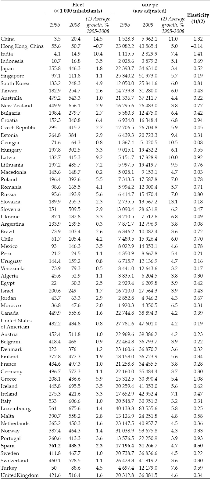
This historic figure was widely surpassed long ago. The Spanish market (see Table 1 in the appendix) reached the amount of 488.3 automobile per 1 000 inhabitants in 2007, a value that has been increasing in the last years but which is far from European standards yet (508 automobile per 1 000 inhabitants in the European Union of 15 member states, EU-15). The features that have been proved to be relevant so far in explaining the long run demand of vehicles are of diverse nature: demographic characteristics of the population, phase of the vital cycle, income, wealth, prices, cost of usage, institutional factors and infrastructures. Among all these variables, when we focus in the long run demand, the main determinant of the degree of motorization is per capita income (Dargay, 2001; Dargay and Getely, 1999). As these authors show, using cross section macro aggregates, the disparities in per capita income explain most of the observed disparities in automobile equipment in cross country studies. A common feature among is the assumption of a lifecycle model in which the income elasticity tends to zero as cars per capita approach to the saturation level of the market. As Greenman (1996) points out, forecasting long run demand depends critically on the value of the estimated saturation level. Due to the lack of time series data long enough, it is very common to estimate such saturation level combining cross section data of income per capita and automobile park density for several countries under alternative assumptions (common saturation level, or country specific saturation if available data allows it). This approach has considerable advantages, but the possible existence of country specific effects or unobservable characteristics (due to lack of data) can introduce undesirable doses of uncertainty in the estimates of the saturation level.
Household characteristics have been typically used in the car market in vehicle type choice models. There are numerous examples of vehicle choice models; including the most recent ones using agent-based modeling (see, for instance, Choo and Mokhtarian, 2004; Kim et al. , 2011; Potoglou, 2008, or Train and Winston, 2007). Berry, Levinsohn and Pakes (2004), for instance, include household characteristics in the estimation of the vehicle type choice in a model of differentiated goods. Their household variables are: household income, number of members in the household, number of adults in the household, age, and a rural dummy. Others have investigated which are the automobile characteristics that make it desirable for the consumer. Requena-Silvente and Walker (2006) study revealed consumer behaviour using a panel data hedonic price estimation strategy. Here, our aim is not estimating vehicle type choice or pricing but total potential demand (quantity) per household in a given market instead.
One of the earlier studies of automobile ownership was the paper by Ben-Akiva and Lerman (1974). They considered several household characteristics as influences on the number of automobiles owned by the household. These are: household income, number of household members, single household dwelling, commuting cost and time, number of autos per number of licensed drivers, car's shopping cost and whether work trip is through the city business district. At that time, they considered the possibility of owning zero, one or two cars. Although some of these variables are out of fashion nowadays, i.e. we do not consider the number of licenses per adults as a restriction any more in developed countries, or the shopping cost is not so much of a restriction either given that there are a wide range of car prices nowadays, (for the choice of car given its price, check the vehicle type choice literature described above), the underlying philosophy of estimating total automobile demand remains.
Our paper shares the same assumptions as in Dargay and Getely (1999) where the growth in car and vehicle ownership is explained as a function of per-capita income. We adopt this view both from a macro point of view, but also from a micro perspective; that is, we assume that household income determines the long run household automobile demand in the same way as the national income affects the long run national demand. This paper goes further in assuming that the saturation level depends on household characteristics, which in aggregate terms affect the countrywide saturation level that usually cannot be taken into account in studies based in macro cross country data. This analysis can be afforded thanks to the availability of the microeconomic database Survey of Household Finances (EFF, Encuesta Financiera de las Familias , in Spanish) elaborated by the Banco de España (Bank of Spain) since 2002. Other studies have used micro data only, like Whelan (2007) for Britain and Matas and Raymond (2008) for Spain. Our paper combines both the traditional approach to the estimation of the saturation level for the automobile market in a pool of 59 countries using macroeconomic data and our proposed complementary approach using micro evidence from Spain.
This double approach allows taking advantage of both types of data: Macro and micro improving the precision of the estimation of saturation levels. Macro data contain observations from countries at different stages of development, so facilitating the estimation of the saturation levels in the automobile market for different levels of per capita income, and thus different stages of the process of diffusion of the automobile. However, there are some country characteristics, such as social, availability of transportation infrastructures, or institutional features, which could affect the saturation level in the market. Micro level data of car ownership within a given country would be unaffected by these sorts of bias in the estimation, and so are very attractive. Moreover, a database with information at the individual or household level would carry a lot more detailed information about the characteristics of the average customer, which should be reflected in the behaviour of the observed households as long as the sample is representative of the society in such country.
BACKGROUND
The differences in income per capita would be able to explain a great deal of the automobile ownership pattern. Although per capita income is one of the main conditionings of the rising tendency in automobile ownership, it does not exist a proved linear relationship between the number of cars and income. In particular, from 1992 onwards the Organisation for Economic Co-operation and Development (OECD) countries have observed a reduction in income elasticity to below-unity levels, while in the 1970s such elasticity was clearly above one. The economic interpretation is that "what once was a luxury good (income elasticity above one) seems to have now become in a necessity (income elasticity below one)" (Dargay, 2001). In the Spanish case, which will concern us later in the paper, Gross Domestic Product (GDP) per capita rose 2.6 percent in the period 1998-2007, while the average number of cars per household suffered a much moderate rise of only 0.1 percent during the same period. This implies that income elasticity in the demand of cars is clearly below one. The motorization rate in the average of the European Union (466 cars per thousand inhabitants in European Union of 27 member states, EU-27) is just slightly above that for Spain (464 cars per thousand inhabitants). Finally, the motorization rate for EU-15 is 508 cars per thousand inhabitants, somewhat above the total EU-27 average.
The level of saturation, defined as the maximum ratio of vehicles with respect to population as income rises is generally determined by long run demand factors. These are potential number of consumers, income and institutional dependent factors, such as infrastructures, population density or urbanization. Although all these factors matter, the most important continues to be income. So, keeping what we have called institutional dependent factors constant, the most adequate variable to measure the level of saturation is income. The level of income per capita summarizes both economic and demographic features in the market, and it is the best single variable to determine what the market potential in a given region is.
Actually, the evolution of income per capita explains most of the behaviour of the automobile market in a country. Likewise, income inequality within a country also explains most of the variation in motorization within the country.
Data compiled in Table 1 in the appendix brings us to some conclusions with respect to the relationship between economic development and vehicle fleet in a country. As can be seen in Figure 1, in general, there is a positive link between GDP per capita growth and motorization. This link is also reflected by the inverse relationship between growth of the vehicle fleet during the period 1995-2008 and the starting levels of GDP per capita in 1995. This reveals that there is a process of convergence in motorization as income rises.
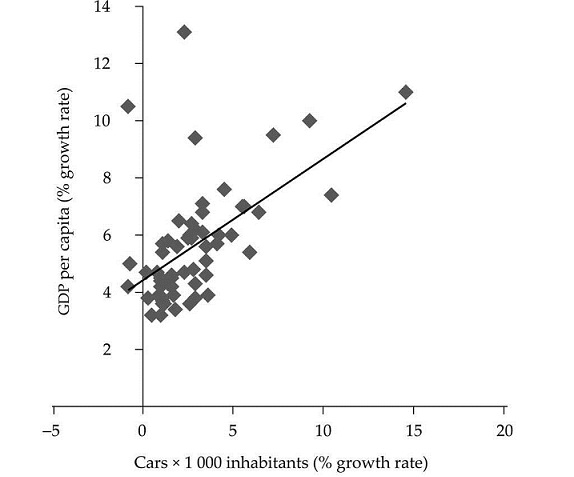
Source: Own elaboration. Data from Euromonitor International, 2009. Available at: < http://www.euromonitor.com/>. List of countries in the Appendix, Table 1A.
Figure 1 Growth of income and vehicles, 1995-2008, for a sample of countries
Data also reflect the non-linear behaviour of income elasticity of automobiles with respect to the starting level of income, measured as the ratio between vehicle fleet growth and income growth (see Figure 2). This feature is widely acknowledged in the literature; it implies that the relationship between vehicle fleet elasticity and income is "bell-shaped". In this way, fleet increases slowly for very low levels of income, faster for higher levels of income, and finally decreases when progressively reaching the level of saturation. These are the characteristics that we want to model explicitly for this market, namely, positive direct relationship with income per capita, the existence of a saturation level in the market and non-linear income elasticity.
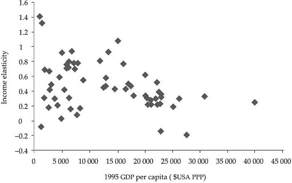
Source: Own elaboration. Data from Euromonitor International, 2009. Available at: < http://www.euromonitor.com/>
Figure 2 Income elasticity of the vehicle fleet and initial level of income per capita. International
METHOD AND THEORY
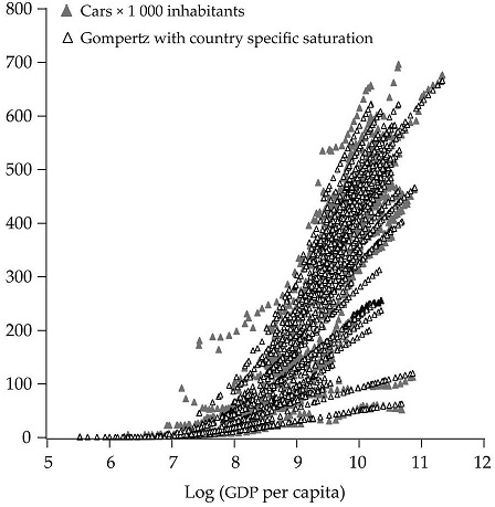
A functional form widely employed in the literature for the estimation of the saturation level of the automobile market is the Gompertz curve. The Gompertz curve was initially presented by Benjamin Gompertz in 1825 and was applied to actuarial sciences (King, 1902), population growth and biology, from modelling growth of Jersey cows (Davidson, 1928) to that of razor clams (Weymouth, McMillin, and Rich, 1931). Raymond Prescott was the first one who suggested the use of the Gompertz curve to model the growth of demand (Prescott, 1922). Recently, it has been applied to the growth potential of the automobile market as in Dargay (2001) for example.
The long run automobile demand function has been estimated, among others, by Greenman (1996) and Dargay and Gately (1999). According to them, the evolution of the automobile density is represented with an S-shape diffusion process, in which motorization density fundamentally depends on income per capita. This type of process captures the main features of automobile demand in the long run: On the one hand, given the exponential functional form, it underlines the existence of an implicit saturation|n level inherent to the nature of the demand in the car market, in such a way that low levels of car density are associated to greater increases in car demand than when approaching the saturation level. On the other hand, this type of functional form captures non-uniformities in income elasticity, which is one of the most relevant characteristics for this product. If we denote as x the automobile demand, and y income, we denote the automobile demand of household c (c , household characteristics) as x c = f (y ,c ).
Since we assume the existence of a saturation level we impose the following restriction,
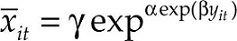
If the long run automobile demand is modelled by means of a Gompertz curve it implies that such level can be represented as:
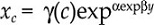 [1]
[1]
where γ(c ) is the level of saturation and depends on the household characteristics, and α < 0 and β < 0 are parameters that define the curvature of the Gompertz function, which have to be estimated using non-linear least squares.
The income elasticity (η) of xc when demand follows a Gompertz curve is given by:
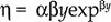 [2]
[2]
which exhibits the previously described demand features in accordance with the characteristics of the pattern of the automobile industry.
Our goal is to obtain estimates of the saturation level using both aggregate (macro) and disaggregate (micro) data. This procedure will lead to a more complete analysis of the automobile market, and it allows us testing the robustness of both estimations. Using microdata has important advantages since it makes possible to include household characteristics (age and sex of the household head, number of household members, etc.), and other variables like the household wealth, that potentially can affect the saturation level, and thus, the long run demand of automobiles. Moreover, the estimated saturation level using micro data will prevent us from the composition effect that can arise when the estimated saturation level is obtained using macro data. This problem was pointed out by Greenman (1996) who warns against the use of cross-section macro data since they prevent from the separation of the three effects that can arise looking at the long run demand of automobile: the diffusion of car ownership, the growth in average income and the dispersion of income.
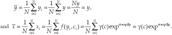
But, as we want to remark in this paper, also the characteristics of the households can have important effects in the estimation of the saturation level. From a macro perspective, if we denote the average per household income as
 [3]
[3]
and /, the average automobile demand per household will be given by:
 [4]
[4]
Clearly, only imposing the very restrictive assumption that all the household are of the same type and they have identical income, we could write2 (suppose that there exist only N household):
 [5]
[5]
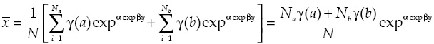
As follows immediately, any departure from such restrictive assumptions will lead to serious bias in the estimation of the saturation level. As can be concluded changes in the income distribution among households and in the characteristics distribution of household will now affect the saturation level. In particular, it will depend of the distribution of household characteristics and their evolution in time. To see this, simply assume that there are only two types of households, say A and B, and that there are N a households of type A, and N b of type B. Assuming that both types of households have the same income but they differ in the long run saturation level, from aggregation equation [4] in discrete terms3 we will have:
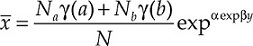 [6]
[6]
So, the countrywide saturation level will become now a weighted mean of the saturation levels of both types of household, and their value will depend on the evolution of the relative size (N a, N b ) of both types of households. We will use equation [6] to come up with the automobile demand saturation level below.
LONG RUN VEHICLE DEMAND
We produce two estimators of potential demand. On the one hand, we estimate the Gompertz curve with aggregate macro data at the national level, using a cross-country international estimation. On the other hand, we estimate the Gompertz curve for the same market (the Spanish case) using micro data coming from the national survey at the consumer level. The purpose is twofold. First, the aim is double-assessing the potential automobile demand for a given national market with data coming from two alternative sources and approaches; and, second, adding a micro-level estimation allows us assessing consumer characteristics, available at the individual household level.
Estimation of the Gompertz curve with aggregate data
We estimate the saturation level coming from an automobile demand function based in the Gompertz curve using a pool of data from all countries in the sample as in Dargay (2001) and Dargay, Gately, and Sommer (2007). Pooling data from all countries together is necessary because it is desirable to have data of all stages of the diffusion process, or in other terms, this is the way to achieve a wide range of values in the observations and match certain levels of economic development to different saturation stages in the automobile market.
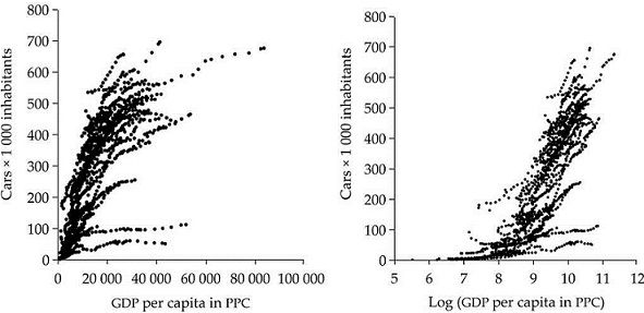
The data used for this application represent the vehicle fleet per 1 000 inhabitants and the GDP per capita in dollars adjusted for purchasing power parity, for the period 1977-2007. The data come from Euromonitor and the set of 59 countries is detailed in Table 2A in the appendix. Figure 3 represents the observed income per capita and car ownership in the pool of all countries. We can observe the tendency of reaching a saturation level for high values of income per capita. Moreover, in general terms, the shape of the figures represented in the graph seems comfortable with assumption imposed about the diffusion process following a Gompertz curve.
In order to estimate the level of saturation of the automobile market we are going to evaluate two alternative models. In the first model we willestimate a common level of saturation for all countries in the sample, which correspond with the more restrictive hypothesis of identical behaviour in all countries. In the second model we will estimate an specific level of saturation for each country by means of fixed effects in γi . The latter model will be relevant in the presence of unobservable country specific factors that can affect long run automobile demand.
In the first model we estimate
 [7]
[7]
Where
The alternative will be as follows:
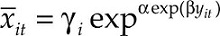 [8]
[8]
Where we estimate γi as an country specific saturation level.
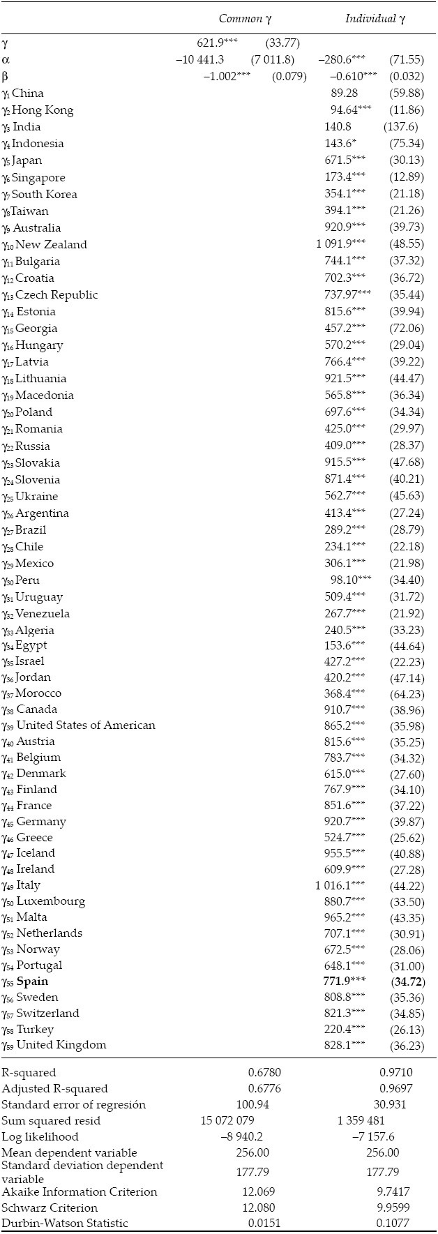
The results of the estimations are presented in the Table 2 of the appendix.
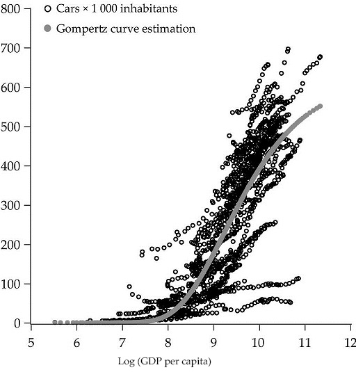
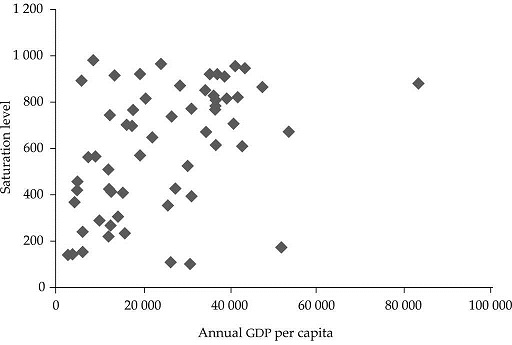
The results of the estimations return a joint saturation level of 621.94 vehicles per 1 000 inhabitants, and a specific saturation level of 771.90 for the Spanish fleet, our case study, (see Table 2 in the appendix for the rest of the countries). As our results show, the estimated country-specific saturation levels show a considerable dispersion. This fact can be explained by the relevance of unobservable factors in the long run demand of automobiles. These unobservable variables cannot be attributed to economic variables, like GDP per capita, since the differences in the estimated saturation level in countries with similar degree of economic development persists. These patterns will make it more appropriate to estimate a country specific level of saturation for the Spanish market, including more information at country level. This will be our case study at the micro level in the second phase.
Estimation of the Gompertz curve with microdata
The Survey of Household Finances (EFF), was first launched by the Banco de España in 2002. The EFF4 is the only statistical source that compiles simultaneously data on household income, assets, debt and spending in Spain. The EFF questionnaire is divided into nine main sections, reflecting the variables studied: Demographics, real assets and their associated debts, other debts, financial assets, pension plans and insurance, labour market status and related income, non-labour income, means of payment and consumption and savings. Among these data, the EEF contains microdata about automobile tenure in the household that we will use to estimate the saturation level of the automobile market from a different perspective, this time taking the household as reference point and unit of observation. Re-estimating the Gompertz curve through this procedure allows us including much more detailed information on the age, sex, and composition in general of the household owning (or non-owning) a car. The data used in this paper corresponds to year 2005, to which we had access, and contains information on 5 962 households.
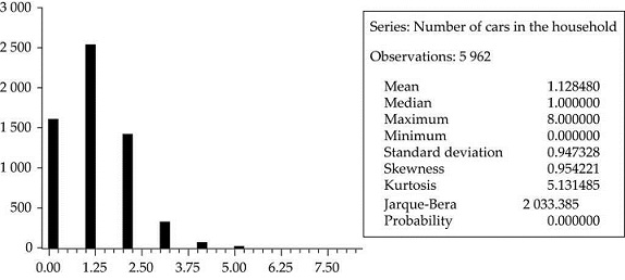
Table 1 describes the structure of the vehicle ownership for the case of Spain according to total household income; age, sex and educational level of the head of household, number of members working in the household and form of house tenure. All these variables may be affecting vehicle demand and are available in the EFF. Initial descriptive statistics reveal that 64.3 percent of the households owning no vehicle are lower income households (below 11 000 euros per year), while two or more cars are more and more common as the income rises beyond 28 000 euros. Owning one car per household is most common in middle-income households (around 20 000 to 40 000 euros), head of household being a male in their thirties with secondary education, and the only working member of the family. We can observe a jump to two vehicles when there are at least two members of the household working. Age is also a determinant factor in the demand of cars. Middle ages are those more prone to become car owners, while non-car owners concentrate in early and late ages (below 30 and above 69 years old). Forms of land tenure seem to affect mainly the choice of purchasing a second car in the house. Households owning a second and a third vehicle are also home owners.
Table 1 Survey of Household Finances, descriptive statistics.
| % of household having (number of cars) | ||||
|---|---|---|---|---|
| 0 | 1 | 2 | 3 and more | |
| Household income | ||||
| < 10.904 | 64.3 | 31.5 | 3.9 | 0.4 |
| 18.632-10.904 | 39.9 | 47.2 | 11.1 | 1.9 |
| 27.797-18.632 | 24.2 | 51.4 | 21.4 | 3.0 |
| 42.730-27.797 | 13.4 | 48.8 | 32.8 | 5.1 |
| 60.945-42.730 | 9.6 | 42.0 | 38.1 | 10.4 |
| > 60.945 | 5.6 | 34.3 | 39.4 | 20.8 |
| Age of household head | ||||
| 18-29 | 31.8 | 45.8 | 18.2 | 4.2 |
| 30-39 | 15.7 | 49.8 | 32.6 | 1.9 |
| 40-54 | 12.5 | 44.7 | 33.7 | 9.1 |
| 55 - 69 | 22.4 | 42.8 | 24.2 | 10.6 |
| 70 and older | 55.3 | 35.0 | 7.7 | 2.0 |
| Sex (household head) | ||||
| Male | 19.1 | 45.7 | 26.8 | 8.4 |
| Female | 37.9 | 37.9 | 19.4 | 4.8 |
| Education (household head) | ||||
| Primary | 37.3 | 40.6 | 17.6 | 4.5 |
| Secondary | 19.0 | 47.6 | 26.5 | 7.0 |
| Tertiary | 13.4 | 41.8 | 33.3 | 11.5 |
| Number of household members working | ||||
| None | 51.5 | 39.3 | 7.8 | 1.4 |
| 1 | 17.4 | 53.6 | 24.5 | 4.5 |
| 2 | 8.4 | 37.9 | 42.3 | 11.4 |
| 3 and more | 5.3 | 24.0 | 35.9 | 34.7 |
| House Tenure | ||||
| Rent | 47.0 | 42.3 | 9.4 | 1.4 |
| Owner | 23.9 | 42.6 | 25.8 | 7.7 |
| Cession | 33.3 | 43.1 | 19.0 | 4.6 |
| Other | 52.9 | 31.4 | 13.7 | 2.0 |
| Household wealth (mean) euros | ||||
| 304 690 | 580 613 | 1 246 211 | 2 692 877 | |
Source: Banco de España. Survey of Household Finances.[Home > Statistics > Other statistics by subject > Survey of Household Finances] Banco de España [online] Available at: <http://www.bde.es/bde/en/areas/estadis/Otras_estadistic/Encuesta_Financi/>.
Robustness tests for the variables in the microdata model: selection of variables
In a first stage we will analyze the variables contained in the EFF5 that may affect household car demand. In doing so, we consider as the independent variable the number of vehicles per household, which can be easily transformed into number of vehicles per 1 000 inhabitants (saturation level) with only a few demographic statistics. Our independent variable, number of cars owned by the household, is a discrete variable which will be modelled with two alternative models: an ordered logit model and a count data model.
The ordered logit model denotes by Ui * the utility perceived by the household i when owning none, one or more cars, and assumes that utility depends linearly on a vector of variables z . So we will have:

If this utility exceeds a certain threshold, ϕi (i = 1,2,..., 8) the household will have respectively no car (if not exceed the threshold), one car (if it exceeds the first but not the second), ..., and up to eight (if exceeds the maximum threshold), which is the maximum number of cars owned by a single household in the sample; i.e.
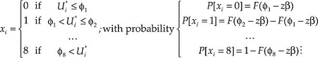
being F(.) the logistic density function.
As a robustness check in the selection of variables, we also run a count data model. In the count data models the conditional mean of the endogenous variable (which can take only positive values or zero) is modelled as a function of some vector of explanatory variables, z , through the expression
It is possible to estimate the parameters using a maximum likelihood estimation method, assuming that the distribution followed by the variable x (number or cars owned by household i ) is a negative binomial variable.
As explained before we check two alternative models for the selection of variables. The first model is an ordered logit and the second is a count data negative binomial. In the two cases the dependent variable is "number of automobiles per household". We include all available variables potentially related to possession of automobiles. These are the following: Age of the head of household, sex, civil status, educational level attained, employment situation, number of working adults in the household, total net income of the household, and home ownership situation. We do not include financial situation due to lack of detailed data on this aspect6. The variables that pass the 5% significance will be used in the saturation level estimation phase.
In short, the estimation procedure is as follows: We test the validity of the variables characterizing the households' car demand using the two alternative models. We then select the variables that are statistically significant in both models. Finally, we use the statistically significant variables in the Gompertz curve estimation to obtain the saturation level of the market.
As expected, the estimation results show that income is positively related to vehicle demand, but the significance of the quadratic term depends on the econometric specification. Higher levels of income always lead to stronger levels of motorization. However, we do not find robust evidence for an inverted U effect, where the automobile is no longer in such demand beyond some level of income. On the contrary, our results suggest that people always like to have one more car. Furthermore, results in Table 2 reveal three basic facts: First, the age of the head of household does not really make a difference, except for households where the head person is over 69 years old. Second, civil status (married, single, divorced, widow/widower) does not make a difference in terms of vehicle ownership. And, third, the educational level does not make a difference either. Additionally, other consumer characteristics that have turned out to be relevant have been incorporated in the final phase of the estimation. These are the following: whether the head of household is a man, less than 70 years old, one adult in the household is working, non-self-employed, and when house is non-rented.
Table 2 Selection of variables estimation results.
| Ordered logit | Count data (negative binomial) | |
|---|---|---|
| Constant | -2.536*** (0.371) | |
| Log household income | 0.102 (0.069) | 0.274** (0.120) |
| Log houhehold income^2 | 0.026*** (0.006) | -0.003 (0.010) |
| Age (reference 18 < age < 30) | ||
| 30 < age < 40 | -0.025 (0.090) | -0.045 (0.115) |
| 40 < age < 55 | -0.065 (0.087) | -0.082 (0.111) |
| 55 < age < 70 | -0.184** (0.091) | -0.167 (0.117) |
| Age >70 | -0.686*** (0.102) | -0.548*** (0.131) |
| Sex (reference male) | ||
| Female | -0.183*** (0.033) | -0.126*** (0.041) |
| Civil status (reference single) | ||
| Married | 0.627*** (0.051) | 0.416*** (0.067) |
| Co-habitation | 0.300*** (0.090) | 0.230** (0.114) |
| Split | 0.162 (0.099) | 0.123 (0.132) |
| Divorced | 0.336*** (0.111) | 0.271* (0.144) |
| Widow/er | 0.024 (0.071) | -0.078 (0.097) |
| Education (reference less than secondary schooling) | ||
| Secondary schooling | 0.109*** (0.039) | 0.078 (0.049) |
| University degree | 0.156*** (0.041) | 0.098* (0.051) |
| Employment situation (reference employed) | ||
| Self-employed | 0.332*** (0.046) | 0.159*** (0.055) |
| Retired | 0.489*** (0.060) | 0.337*** (0.074) |
| Unemployed or inactive | 0.397*** (0.062) | 0.211*** (0.079) |
| Working adults in the household (reference none) | ||
| One | 0.769*** (0.052) | 0.538*** (0.066) |
| Two | 1.051*** (0.063) | 0.653*** (0.077) |
| Three or more | 1.633*** (0.084) | 0.918*** (0.099) |
| Housing tenure (reference renting) | ||
| Owner | 0.684*** (0.056) | 0.454*** (0.075) |
| Cession | 0.653*** (0.083) | 0.428*** (0.109) |
| Other | 0.383** (0.185) | 0.228 (0.249) |
| Log likelihood | -5 906.9 | -8 180.6 |
| LR statistic (23 df) | 3 476.8 | 1 067.9 |
| Probability(LR statistic) | 0.0000 | 0.0000 |
| Limit points Ordered logit | Limit points Ordered logit | ||
|---|---|---|---|
| Limit 1 | 2.183*** (0.222) | Limit 5 | 6.615*** (0.240) |
| Limit 2 | 3.820*** (0.225) | Limit 6 | 7.063*** (0.257) |
| Limit 3 | 5.150*** (0.228) | Limit 7 | 7.449*** (0.292) |
| Limit 4 | 6.037*** (0.231) | Limit 8 | 7.965*** (0.404) |
Notes: Standard errors in parenthesis. * 90% confidence level, ** 95% confidence level, ***99% confidence level.
Estimation of the Gompertz curve
In the last section, we have seen which household characteristics are significant. These are the characteristics that are used in the following model. In this second phase we estimate the saturation level with micro data using the Gompertz curve specification that follows:
 [9]
[9]
Where γ0 is the level of saturation for a reference household (no adult household member works, male head, head aged over 69, house is not rented) and γ1 is total household income. Parameters γ1, γ2, γ3, γ4, γ5, γ6, γ7, γ8 and γ9 underpin the differential effect of the head of household being under 70; being a woman; one or more adults working in the household; being active (self-employed or employee), and living in a rented house. Parameters α and β capture the curvature and slope of the Gompertz curve.
The next Table and Figure present the results of the estimation.
Table 3 Gompertz curve estimation results.
| Variable | Coefficient (standard error) |
|---|---|
| Reference (no adult household member works, male head, aged over 70, house is nor rented) | 1.837*** (0.244) |
| One adult household member working | 1.184*** (0.186) |
| Two adult household member working | 1.802*** (0.269) |
| Three or more adult household member working | 2.823*** (0.404) |
| Head self-employed | -0.193* (0.097) |
| Head employee | -0.735*** (0.127) |
| Head female | -0.407*** (0.073) |
| Head aged under 70 | 0.783*** (0.128) |
| House is rented | -1.116*** (0.174) |
| α | -5.095*** (0.720) |
| β | -0.298*** (0.049) |
| R-squared | 0.4035 |
| Adjusted R-squared | 0.4025 |
| Standard error of regression | 0.7327 |
| Sum squared residuals | 3 166.7 |
| Log likelihood | -6 542.1 |
| Mean dependent variable | 1.1333 |
| Standard deviation dependent variable | 0.9479 |
| Akaike Information Criterion | 2.2176 |
| Schwarz Criterion | 2.2301 |
| Durbin-Watson Statistic | 1.9875 |
For a reference household our estimation results show a saturation level of 1.84 cars per household, which increases with the number of adult household member working7 and when the head of household is aged under 70 years. In contrast, when the head of household is a female, or when the house is rented, the saturation level decreases. These figures are slightly under the saturation level obtained with macro data (771.9 cars per 1 000 inhabitants). Following the data of the Instituto Nacional de Estadística (INE) [National Institute of Statistics]8, we can establish that in Spain the most frequent situation is a household formed by two adults under 65 (with no children, or with less than three children), where the reference person is a male, where both adult members work (employed) or only one of them, and that housing rental is marginal. According to these figures, we plug the estimated parameters in equation [6] in order to obtain the saturation level. Thus, we can conclude that the saturation level in Spain arising from microdata amounts to 724 cars per 1 000 inhabitants.
Table 4 Average number of people per household by sex and age of head of household.
| Number of households | People | Saturation level at X cars | |
|---|---|---|---|
| Total | 11 986 305 | 35 818 959 | |
| Total males | 741 752 | 1 841 945 | |
| Males between 16 and 29 years old | 4 020 227 | 12 601 568 | |
| Males between 30 and 44 years old | 4 560 489 | 15 164 553 | 2.286 b/ |
| Males between 45 and 64 years old | 2 663 837 | 6 210 893 | |
| Males 65 years old and above a/ | 11 986 305 | 35 818 959 | 1.837 |
| Total Females | 3 869 289 | 8 015 830 | 1.431 c/ |
| Total | 15 855 594 | 43 834 789 |
Notes: a/ There is not data available for head of household aged 70 years and over. We assume that 65 years and over is equivalent to 70 years and over. b/ Is the result of 1.837+1.184-0.73. c/ Is the result of 1.837-0.40.
Source: INE. Household Budget Survey. [INEbase > Standard and life conditions (CPI) > Living conditions > Household Budget Survey] INE[online] Available at: <http://www.ine.es/dyngs/INEbase/>.
CONCLUSIONS
We have seen that using a dual approach for the estimation of the saturation level of automobile market can improve our knowledge about the long run dynamics of car penetration. Using microdata improves the quality of the estimates of the saturation level since it enables to include household characteristics (age and sex of the household head, number of household members, etc.), and other variables that potentially can affect the household car demand, and thus, the long run demand of automobiles. Our results show that the use of cross section macro data could hide important characteristics with notable impact on long run demand. This is the case of the negative effect of ageing population on market saturation levels which can push down the demand of automobiles in developed countries as is the case of Spain. This effect is masked when cross section data of developing and developed countries with different population age structures are employed. Similarly other factors like the household size, the number of adult household members working or the sex of the household head are statistical significant in explaining the saturation level of the Spanish automobile market, and thus, their omission will lead to biased estimates of the saturation level.
If we compare the saturation level estimators obtained from the two alternative estimation approaches, it is remarkable how close they are. We indeed obtain similar results with both macro and micro approaches and, most importantly, they complement each other. Each one is proving different types of relevant information on automobile demand. The macro approach gives us an international cross-country comparison given the income level, while the micro approach provides detailed household features of automobile demanders.