Real business cycles in emerging economies: the role of international growth and interest rate

 

Ciclos económicos reales en economías emergentes: el papel del crecimiento y la tasa de interés internacional

 

Francisco Venegas-Martínez*, Raúl O. Fernández** and J. Eduardo Vera-Valdés***

 

* Escuela Superior de Economía del Instituto Politécnico Nacional (ES-IPN). Correo electrónico: <fvenegas1111@yahoo.com.mx>.

** Banco de México (Banxico). Correo electrónico: <rfernandez@banxico.org.mx>.

*** Correo electrónico: <eduardo@cimat.mx>.

 

Received August 2010.
Accepted November 2011.

 

Abstract

This paper is aimed at developing a business-cycle model for a small open emerging economy (SOEE). The model is parameterized, calibrated, and simulated to rationalize two important stylized facts in a SOEE. The first one is that when the international interest rate increases, the growth rate of a SOEE is reduced. Secondly, when industrialized countries are in recession, a SOEE suffers an even larger reduction in their growth rate. The obtained results show that if exports respond negatively to the international interest rate or exports are reduced due to an international recession, the aggregated consumption of the domestic economy is substantially more volatile than an economy where exports do not react. Moreover, this paper provides a possible explanation to the puzzle that developing countries suffer a recession not only when industrialized countries are in recession, but also when they are growing too fast.

Key words: real business cycles, emerging economies, international growth, international interest rates.

JEL Classification:* F43, E32, E44.

 

Resumen

Este trabajo desarrolla un modelo de ciclo económico para una economía pequeña, abierta y emergente (EPAE). El modelo es parametrizado, calibrado y simulado para explicar dos hechos estilizados importantes en las EPAEs. El primero es que cuando la tasa de interés internacional se incrementa, la tasa de crecimiento de las EPAEs se reduce. El segundo es que cuando los países industrializados están en recesión, las EPAEs sufren una reducción en sus tasas de crecimiento aún mayor que los países industrializados. El principal resultado es que si las exportaciones responden negativamente a la tasa de interés internacional o se reducen como consecuencia de una recesión internacional, la EPAE tendrá una mayor volatilidad en su consumo agregado que una economía donde las exportaciones no reaccionan de esa forma. Además, este trabajo proporciona una posible explicación al aparente enigma de que los países en desarrollo sufren una recesión no sólo cuando los países industrializados tienen una recesión, sino también cuando crecen demasiado rápido.

Palabras clave: ciclos económicos reales, economías emergentes, crecimiento internacional, tasa de interés internacional.

 

INTRODUCTION

There are two important stylized facts that business cycles in small open emerging economies (SOEEs) have experienced in the last decades. The first one is a negative correlation between output and the cost of borrowing that these countries face in international financial markets. Secondly, there is a positive correlation between output and moderate international growth rate. Periods of low international interest rate and moderate growth rate in the international economy are often associated with economic expansions in emerging economies and periods of high international interest rate or negative growth rate in the international economy are associated with economic recessions in SOEEs.

For example, in the 90's, when the Federal Reserve increased its Federal Fund Rate, while United States was having a moderate stable growth rate, SOEEs experienced a slowdown in their growth rates. More recently, even though the Federal Reserve has reduced its Federal Fund Rate since the beginning of the global financial crisis that started in United States in 2007, SOEEs have seen a larger reduction in their growth rates compared with industrialized countries.

Uribe and Yue (2006) investigated the relation between international interest rates, country spreads, and output fluctuations in a sample of seven emerging economies (Argentina, Brazil, Mexico, Peru, Philippines and South Africa). They found a strong negative correlation between real interest rates and economic activity. Moreover, they found that in response to an increase in United States interest rates, country spreads first fell and then displayed a large, delayed overshooting. This affects domestic variables mostly through their effects on country spreads, following then a feedback from emerging-market fundamentals to country spreads, significantly exacerbating business-cycle fluctuations.

In another work, Neumeyer and Perri (2005) perform a statistical analysis of business cycles in a set of SOEEs (Argentina, Brazil, Mexico, Korea, and Philippines) and in a set of small open developed economies (Australia, Canada, Netherlands, New Zealand, and Sweden). They find that many features of business cycles are similar between the two sets of economies, but that there are also some notable differences. Particularly, in emerging economies real interest rates are countercyclical and lead the business cycle. In contrast, real rates in developed economies are acyclical and lag the cycle.¹ These authors lay out a model that is helpful in understanding and quantifying the nature of such a relationship. In their model they assume that country spreads are exogenous to domestic conditions in emerging countries. Specifically, they assumed that the country spread and the United States interest rate follow a bivariate first-order autoregressive process. They estimate such a process and use it as a driving force of a theoretical model calibrated to Argentine data. In this way, Neumeyer and Perri assess the mechanism by which interest rates exacerbate aggregate consumption volatility in developing countries.

In contrast, many authors, like Edwards (1984), and Cline and Barnes (1997) have documented that country spreads respond systematically and counter-cyclically to business conditions in SOEE's. They find that domestic variables such as Gross Domestic Product (GDP) level, GDP growth and exports growth have a significant impact on the country risk in developing economies. Cantor and Packer (1996) and Eichengreen and Mody (2000) have documented that higher credit ratings, which, in turn, have been found to respond strongly to domestic macroeconomic conditions, translate into lower country spreads.

Following Neumeyer and Perri (2005), we develop a dynamic stochastic general equilibrium model (DSGE) for a SOEE where the interest rate is decomposed into an international rate and a country risk component. It is important to point out that we introduce a couple of modifications as in Neumeyer and Perri's (2005) model, in a standard neoclassical framework, to build a business cycle model that is consistent with the main empirical regularities of emerging economies. The first modification is that firms have to pay for part of the factor of production before it takes place, creating a need for working capital. The second one, which is common in the small open economy literature, is that we consider preferences which generate a labor supply that is independent of consumption. These two modifications generate the transmission mechanism by which real interest rate affect the level of economic activity. In addition to Neumeyer and Perri's (2005) model, ours introduces an exogenous export demand that depends on the international real interest rate and on an international recession rate.

One of the main findings from this research is that if exports respond negatively to the international interest rate or to an international recession, the aggregated consumption of the domestic economy is substantially more volatile than an economy where exports do not react. In other words, this paper finds a coherent explanation to the riddle when either industrialized countries are growing too fast or face a recession, developing countries suffer.

The paper is organized as follows. Section 2 presents the model with the inclusion of an equation for exports to the economy. Section3 discusses some impulse responses to the model among a simulated economy based on our model. Finally, section 4 concludes with an emphasis on the Mexican and Argentine cases.

 

THE SETTING OF THE ECONOMY

Assume a small open economy populated by identical households. Also, assume that this economy has two sectors, one of which includes firms producing tradable goods and the other producing non tradable goods. Each sector has a continuum of monopolistic competitive firms indexed by t ∈ [0,∞). Finally, it is assumed that there is a monetary authority.²

In this model, the law of one price holds for internationally tradable goods. That is, P_t^T = ε_t P_t^T* for all t ∈ [0,∞) periods where P_t^T and P_t^T* denote the nominal price of the tradable goods in the domestic and foreign economies, respectively, and ε_t is the nominal exchange rate (in domestic currency per unit of foreign currency). Moreover, normalizing the foreign price of tradable goods to one, the law of one price implies P_t^T*= ε_t. The nominal price index of non tradable goods is P_t^N, and is the gross inflation rate of non tradable goods. We define the real exchange rate e_t as the relative price of tradable goods in terms of non tradable goods, that is, e_t= ε_t /P_t^N.

The idea behind this assumption is that identical goods sold in different countries must sell for the same price when their prices are expressed in terms of the same currency. If not, then an arbitrageur will purchase the good in the cheaper market and sell it where prices are higher. Nonetheless, it is important to note that this law applies only in competitive markets free of transport costs and barriers to trade.³

So far we have assumed that the economy has two sectors producing tradable⁴ and non tradable goods, respectively. A firm, in the former sector, can borrow from the rest of the world at the international real interest rate plus the country-risk premium, Q(·),⁵ but a firm, in the latter sector, can only borrow from local households at the domestic interest rate which is equal to the international interest rate plus the country risk premium Q(·) plus the expected depreciation of the exchange rate. Following Neumeyer and Perri (2005), we assume that the premium is inversely (negatively) related to the technology shocks (specified below) but we add exports as a new argument, thus the domestic nominal interest rate satisfies:⁶

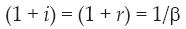
that is, the domestic nominal interest rate (1 + i_t) equals the exogenous real international interest rate (1 + r_t) adjusted by the expected country-risk premium 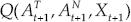and adjusted by the expected depreciation rate.

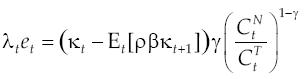
We suppose that the country risk premium has the following functional form:

with σ, ς, τ > 0 and where A_t^j {j = T, N} is a technology shock specified below. That is, the country risk premium is a function of the technology shock in the tradable and non tradable firms and in exports. Note that when σ = ς = τ = 0, the country-risk premium is eliminated and the condition above boils down to the standard uncovered interest rate parity condition.

The international real interest rate is exogenous to the SOEE, as the deinition of small economy implies, and it will be assumed that it follows the following autoregressive process:

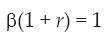
where Φ_r∈ (0,1) and ln(ξ_rt)~WN(0,1), that is ln(ξ_rt) is a white noise process with zero mean and unitary variance. The term (1/β)^1Φr appears in the above equation since, following Schmitt-Grohé and Uribe (2003), we assume that in the steady state β(1 + r) = 1. Here β is the subjective discount factor of the (representative) individual. Note that this assumption was made to eliminate any trend in real variables.

Consumers

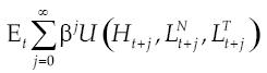
The representative household derives utility from leisure and consumption of a basket of goods containing a homogeneous tradable good C_t^T and a variety of heterogeneous non tradable goods C_t^N (z), where z ∈[0,1] corresponds to the index of the producing firm. As in Uribe (2002), the model allows for the formation of habit in consumption.

We consider the household's utility function, first proposed by Greenwood Hervicotz and Huffman (1988), given by:

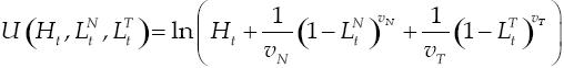
where: H_t= C_t - ρC_t-1.

Here ρ∈[0,1) is the habit parameter, L_t^J {j = T, N} is time allocated to labor with the total endowment of time per period normalized to one, and V_N and V_T are preference parameters. Moreover, C_t is a composite basket of tradable and non tradable goods defined by:

Households hold nationally traded bonds denominated in units of nontradable goods b_t, which yield a real domestic interest rate i_t. Sources of funds in period t include: the principal and the return of bonds purchased at time t - 1, b_t-1(1 + i_t-1), remunerations from labor at nominal wages rate W_t^j {j = T, N}, and lump-sum transfers equal to the aggregate firm' nominal profits, denoted by Δ_t^j {j = T, N}.

The use of funds consist of consumption of the homogeneous tradable good C_t^T, consumption of non tradable goods C_t^N (z) with nominal price p_t^N (z) for z ∈ [0,1] and new issued bonds b_t. The agent's budget constraint in terms of non tradable goods is

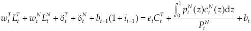
where

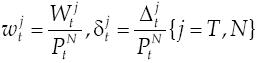
At each time t, the household chooses and b_t to maximize

subject to the budget constraint and the aggregators. Cost minimization implies the demand for the variety z:

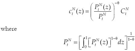
is the utility-based price index. Let λ_t denote the Lagrange multiplier, the first order conditions for an interior solution implies:

The above expression says that, at the optimum, the marginal rate of substitution between non tradable and tradable goods must be equal to relative prices, that is, the real exchange rate. Notice also that

where

The first order condition with respect to H_t is given by: H_t = C_t - ρC_t-1, which simply states aggregate consumption with habit.

The above equation stands for the aggregate consumption of both tradable and non tradable goods. We also have:

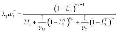
This expression is the standard Euler equation. Moreover, a relationship between the multiplier λ_t and w_t^N can be stated as:

This equation is the labor supply curve for the non tradable firms. It says that, at the optimum, the consumer equals the marginal utility of a unit of leisure with the marginal utility of consumption that his salary allows him to purchase. In the same way,

This equation is the labor supply curve for tradable firms. Finally, by collapsing the above results, we obtain:

This equation rewrites the consumer's budget constraint.

The non tradable firm

Following Calvo's (1983) pricing, the model assumes that there is a continuum of firms that change prices in a staggered fashion. They do this only when they receive an idiosyncratic random signal that arrives with probability 1 - α; such probability is supposed to be constant in every period of time, independent of the state of the economy. The producer z has access to the technology

Where A_t^N is a technology shock of the non tradable sector, which follows the process:

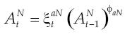
with ln (0,1) and Φ_aN ∈(0,1).

Since the technology is the same for all producers we can drop the index z. As in Neumeyer and Perri (2005), the firm is subject to a working capital constraint for which it has to borrow the fraction μ^N∈[0,1] of its nominal marginal cost Ψ_t.

The firm pays the interest i_t for the loans. Thus the effective nominal marginal cost is Ψ_t(1 + μ^Ni_t) and the effective real marginal cost becomes 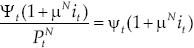where Ψ_t is the real marginal cost.

The producer profit in terms of the non tradable goods satisfies:

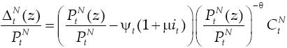
where c_t(z) is given by the demand and the real marginal cost in terms of non tradable goods, and Ψ_t is given by the production technology. Note that when μ = 0, the model boils down to the standard model without working capital.

The producer chooses P_t^N (z) to maximize:

where βjΩ_t,t+j is the relevant stochastic discount factor between t and t + 1.

Optimal price

By solving the producer's decision problem, the firms' optimal price is given by:

Notice that this price depends on the real marginal costs in terms of non tradable goods, the elasticity of non tradable goods, the discount factor, and the signal probability.

Price index ofnon tradable goods

By using Calvo's (1983) structure, we can aggregate prices by using a simple recursive equation:

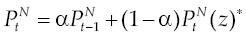
This says that the current price, in the non tradable sector, is a weighted average between the past price and the optimal current price.

The tradable firm

We assume that the firm producing the tradable good has access to a technology of the form:

where A_t^T is a technology shock of the tradable sector, which is driven by the following process:

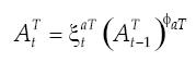
with In~ WN(0,1) and Φ_aT ∈(0,1).

The firm maximizes its dividends in non tradable goods, that is:

subject to its technology. The domestic demand for tradable goods and the demand of exports satisfy:

We are assuming that the tradable firm faces the international interest rate plus the risk premium. The underlying idea is that even though it has access to the international financial market, it is still exposed to the risk associated to its country. In this case, the first order condition is given by:

Note that we distinguish between technology shocks for tradable and non tradable firms. We also allow the possibility for different working capital restrictions for each sector.

Country risk premium and exports

As before, we are assuming that the country risk premium is inversely related to both the expected demand of export and the expected technology shocks affecting both sectors. This assumption seeks to model the well-documented fact that the fundamentals, captured here by exports, impact on the country risk premium. In this case, we may provide a plausible interpretation of a negative export shock as a negative growth rate in the global economy. At the same time, we are assuming that the international interest rate affects negatively the demand for exports of the emerging economy. Therefore, the demand for exports satisfies:

with ln~ WN(0,1) and Φ_xr ∈(0,1). Note that different values for Φ_xr would dampen or amplify the reaction of the main variables of this economy.

Monetary authority

The Central Bank maneuvers the interest rate following a rule that responds to deviation of inflation in non tradable goods from its steady state equilibrium much in line with the one proposed by Taylor (1993). Central Bank authorities are also concerned with smoothing the interest rate (see Clarida, Gali and Gertler, 2000). In this case, the monetary authority acts by using a generalized Taylor's rule:

where

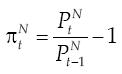
is the inflation rate in the non tradable sector. We assume that in steady-state π = 0, which implies

The shock to the monetary rule follows the process: I_t = ξ_It(I_t_₁)^ΦI, where ln(ξ_It)~WN(0,1) and Φ_I∈(0,1).

 

STEADY STATE AND IMPULSE RESPONSES

In this section, as in Kydland and Prescott (1982), we examine the behavior of the proposed economy. To do this, we analyze different shocks and different values for the concerned parameters. In particular, both exports demand and interest rate shocks will be considered.

Steady state

The steady state stands for the equilibrium towards which, in absence of shocks, the economy converges. In this economy, as we have previously assumed

so that the real variables do not have a trend. Consequently, in steady state

for all t, and so on, where the symbol "o" denotes the steady state values of relevant variables. Notice that there is not an ongoing structural change (shifts across sectors) at the steady state.

Deviations from the steady state

The impulse responses are calculated as deviations from the steady state, and are calculated by using the parameter values summarized in table 1. We have chosen α = 0.75 so that, on average, firms reset prices every quarter. The parameter value γ = 0.5 indicates that the consumption bundle is comprised of half tradable goods and half non tradable goods. The reaction coefficients of the Taylor rule are σ_i = 0.5 and σ_π = 0.6 so that the rule satisfies the conditions so that there is a unique equilibrium. Finally, μ_T and μ_N are chosen so that firms must pay in advance 75% of their marginal cost.

Exports shock

In what follows, we analyze the response to exports demand shocks. Figure 1 shows the impulse response given a negative shock to the demand of exports.⁸ This shock increases the country risk premium, which tends to raise the domestic interest rate but, at the same time, lowers the inflation rate. As our central bank follows the generalized Taylor rule, the consequence of this movement in the inflation rate is that the domestic interest rate actually goes down over-killing the initial stimulus to go up. In turn, the lower level of exports causes a lower demand for labor in the tradable sector. As we are allowing perfect substitution between tradable and non tradable labor, it follows that more workers are hired in the non tradable sector. As a result, the consumption in the non tradable sector goes up and it goes down in the tradable sector. The fall of consumption in the tradable sector is bigger, in absolute value, than the fall in exports demand. Finally, the figure shows that the aggregated consumption has fallen as empirical evidence suggests.

International interest rate shock

Next, we study the effects on our economy of shocks in the international interest rate. Figure 2 shows the impulse response, given a shock to the international interest for different values of the elasticity of exports to the international interest rate. As we have assumed, the increase in the international interest rate leads to a downward in the exports demand. This is the case because we have assumed that exports are negatively related to the international interest rate. An increase in the international interest rate ceteris paribus tends to increase the domestic interest rate not just as a result of the shock by itself, but also as a result of the increase in the country risk premium, as we have explained before. Once the shock hits the exports demand the dynamics of the economy is qualitative similar to the dynamic presented in the previous shock.

As figure 2 suggests, a key parameter in this economy is the elasticity of exports demand to the international interest rate. Different values of this parameter will amplify or dampen the dynamics of this economy.

Figure 3 shows a simulated economy for which the exports demand do not depend of the international interest rate. Figure 4 shows basically the same economy but with an elasticity of exports demand to the international interest rate equal to 2.5.

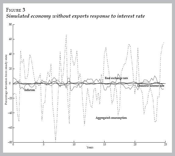
As we have pointed out before, this parameter plays a key role in the aggregated consumption volatility of the economy. Observe that with Φ_xr = 2.5 the aggregated consumption volatility is almost twice as in the zero elasticity case.

 

CONCLUSIONS

In this paper we have studied the international interest rate and the global growth rate channel to fluctuations through the exports demand. To reach this goal we introduced the role of exports demand in a SOEE in a simple fashion. The model shows that the elasticity of exports demand to the international interest rate could explain a higher aggregated consumption volatility in SOEEs. We find two important results. First, if the international growth rate is negative, the SOEE will experiment an even bigger decrease in its activity. Secondly, a small increase in the international interest rate could produce a substantially higher volatility in aggregated consumption in the SOEE, provided exports elasticity becomes bigger.

At the same time, our proposed model could provide an explanation of the events observed in the last two decades. In particular, in the 90's, when the Federal Reserve Board increased the Federal Funds Rate, Mexico and Argentina experienced worse conditions in their financial markets, joint with a reduction in their growth rates.

This model also helps explain the events observed in the last financial crisis. Even though the Federal Reserve Board reduced the Federal Funds Rate after the recession in the United States economy, the reduction in exports implied an even bigger reduction in the growth rate in Mexico and Argentina.

Two important policy implications are in order. The first one is that it is very important to diversify exports, by including more countries and goods, so that the risk of a big adverse shock in the export is reduced. The second one is a SOEE should develop their own domestic market in order to mitigate their exposition to external shocks.

As usual, some caveats apply. In the first place, we have not considered the imports demand sector that could cause some feedbacks between the economies. On the second place, it would be desirable to include some rigidities to the substitution of labor among the tradable and non tradable sectors.

 

Appendix

 

REFERENCES

Blanchard, O. and Miles-Ferreti, G.M., 2010. Global imbalances: in midstream? In: O. Blanchard and I. SaKong, eds. Reconstucting the World Economy. Washington: International Monetary Fund (IMF).         [ Links ]

Burstein, A., Neves, J.C. and Rebelo S.T., 2003. Distribution costs and real exchange rate dynamics during exchange-rate-based stabilizations. Journal of Monetary Economics, 50(6), pp. 1189-214.         [ Links ]

Cantor, R. and Packer, F., 1996. Determinants and impact of sovereign credit ratings. Economic Policy Review, 2(2), pp. 37-53.         [ Links ]

Calvo, G.A., 1998. Capital flows and capital-market crises: the simple economics of sudden stops. Journal of Applied Economics, 1(1), pp. 35-54.         [ Links ]

Calvo, G.A., 1983. Staggered prices in a utility-maximizing framework. Journal of Monetary Economics, 12(3), pp. 383-98.         [ Links ]

Clarida, R., Galí, J. and Gertler, M., 2000. Monetary policy rules and macroeconomic stability: evidence and some theory. Quarterly Journal of Economics, 115(1), pp. 147-80.         [ Links ]

Cline, WR. and Barnes, K.S., 1997. Spreads and risk in emerging market lending. Institute of International Finance (IIF) Research Paper no. 97-1. Washington, DC: IIF.         [ Links ]

Dornbusch, R., 1987. Exchange rates and prices. American Economic Review, 1(77), pp. 93-106.         [ Links ]

Edwards, S., 1984. LDC foreign borrowing and default risk: an empirical investigation. American Economic Review, 74(4), pp. 726-34.         [ Links ]

Eichengreen, B. and Mody A., 2000. What explains changing spreads on emerging-market debt: fundamentals or market sentiment? In: S. Edwards, ed. The Economics of International Capital Flows. Chicago: Chicago University Press.         [ Links ]

Greenwood, J., Hervicotz, Z. and Huffman, G.W, 1988. Investment, capacity utilization, and the real business cycle. American Economic Review, 78(3), pp. 402-17.         [ Links ]

Kydland, F. and Prescott, E., 1982. Time to build and aggregate fluctuations. Econometrica, 50(6), pp. 1345-71.         [ Links ]

Krugman, P., 1987. Pricing to market when the exchange rate changes. In: S.W Arndt and J. Richardson, eds. Real Financial Linkages Among Open Economies. Cambridge, MA: MIT Press.         [ Links ]

Neumeyer, P.A. and Perri, F., 2005. Business cycles in emerging markets: the role of interest rates. Journal of Monetary Economics, 52(2), pp. 345-80.         [ Links ]

Schmitt-Grohé, S. and Uribe, M., 2003. Closing small open economy models. Journal of international Economics, 6(1), pp. 163-85.         [ Links ]

Taylor, J.B., 1993. Discretion versus policy rules in practice, Carnegie-Rochester Conference Series On Public Policy, 39, pp. 195-214.         [ Links ]

Uhlig, H., 1995. A toolkit for analyzing nonlinear dynamic stochastic models easily. Institute for Empirical Macroeconomics Discussion Paper no. 101. Minneapolis: Federal Reserve Bank of Minneapolis.         [ Links ]

Uribe, M., 2002. The price-consumption puzzle of currency pegs. Journal of Monetary Economics, 49(3), pp. 533-69.         [ Links ]

Uribe, M. and Yue, V.Z., 2006. Country spreads and emerging countries: who drives whom? Journal of International Economics, 69(1), pp. 6-36.         [ Links ]

 

NOTAS

* JEL: Journal of Economic Literature-Econlit.

The opinions expressed in this paper are exclusively those of the authors and do not necessarily reflect the view of Banco de México. The authors thank the comments and suggestions made by anonymous referees which improved this work. As usual any remaining errors are the solely responsibility of the authors.

¹ They also find that emerging economies display high output volatility, relative to developed economies. Moreover, the volatility of consumption relative to income is on average greater than one, and higher than that in the developed economies. Finally, net exports appear much more strongly countercyclical in emerging economies than in developed ones.

² Note that we are simplifying as much as possible in order to focus in the role of international growth and interest rate in the business cycles in a SOEE. We are aware that some of the assumptions do not correspond exactly with real economies, even though these assumptions are widely used in the literature as benchmarks and will prove to be useful in this work.

³ Furthermore, the law of one price may not hold for various reasons including demand elasticity as it has been emphasized in numerous studies on pricing including the early contributions by Dornbusch (1987) and Krugman (1987). Another standard approach to account for deviations from the law of one price in the literature is based on location specific costs. All tradable consumer goods that are highly tradable embody non-tradable costs of distribution, such as labor costs at retail stores and rental costs of operating space. In this respect, Burstein, Neves, and Rebelo (2003) have reported that the distribution margin represents more than 40% of the final good price.

⁴ In the case of the Mexican economy, we may think of a commodity sector including Petróleos Mexicanos (PEMEX), while in the Argentine economy we may think of the agricultural sector.

⁵ This assumption follows from the fact that a firm that produces the tradable good is a domestic one, so even though its sales are made in foreign currency, it cannot escape from paying the country-risk premium

⁶ Recall that we are concerned with net borrower economies —Argentina and Mexico— and riskier than the big economies —England, United States, Germany and Japan—. It is natural to assume that the domestic interest rate is positively correlated with the international interest rate because an imbalance of the domestic interest rate from the international interest rate would imply destabilizing flows of capital like sudden stops in international credit flows (see Calvo, 1998), or unsustainable imbalances (see Blanchard and Miles-Ferreti, 2010).

⁷ The values of the parameters are not chosen to model any particular economy but a synthetic one as a means to evaluate the implications of our model.

⁸ This shock may be interpreted as a change in the demand of a small open economy exports due to a change in the preferences abroad, or more interesting it could be a cause of a recession in the big economy. Either way, it reduces exports of the small open economy, this, in turn, worsens the fundamentals, augmenting the country-risk premium.