


Services on Demand
Journal
Article
 English (pdf)
 Article in xml format
 Article references
 Send this article by e-mail
Indicators
-
 Cited by SciELO
 -
 Access statistics
Related links
-
 Similars in
SciELO
Similars in
SciELO
Share

 Permalink
Investigación económica
Print version ISSN 0185-1667
Inv. Econ vol.70 n.277 Ciudad de México Jul./Sep. 2011
Quantitative easing: a Keynesian critique
Relajación cuantitativa: una crítica keynesiana
Thomas I. Palley*
New America Foundation, <mail@thomaspalley.com>.
Received April 2011
Accepted June 2011.
Abstract
Keynesian economists have generally supported quantitative easing (QE) on grounds it increases aggregate demand and anything that increases demand at this time of demand shortage is welcome. This paper argues that response may be misplaced. QE may back fire with respect to demand stimulus create potentially significant future dangers, and is supportive of a plutocratic based on "asset market trickle-down" that obstructs needed policy change.
Key words: quantitative easing, monetary policy, asset prices.
Clasificación JEL: ** E43, E44, E50, E52, E58.
Resumen
Los economistas keynesianos han apoyado de manera general la relajación cuantitativa (QE por sus siglas en inglés) por la razón de que incrementa la demanda agregada y que cualquier cosa que la incremente en estos tiempos de escasez de demanda es bienvenida. Este artículo se argumenta que esta respuesta puede estar equivocada. La QE puede tener efecto boomerang con respecto al estímulo de demanda, crear peligros potenciales significativos en el futuro y favorece una economía política plutocrática basada en un "filtro de mercado de activos" que obstruye el necesario cambio de política.
Palabras clave: relajación cuantitativa, política monetaria, precios de activos.
INTRODUCTION
The Great Recession of 2007-2009 has seen the Federal Reserve push the federal funds rate to almost zero, hitting the so-called zero bound. In light of this condition the Federal Reserve has engaged in two rounds of quantitative easing (QE), a policy whereby a central bank buys long-term government bonds and private sector financial assets (particularly mortgage related products).
The policy of QE has been supported by new Keynesians (see for example Krugman 2010, De Long 2009 and Farmer 2009), and it also appears to have the support of traditional Keynesians and Post Keynesians. Balanced against this, it has been criticized by both monetarists (Meltzer 2011) and new classical macroeconomists (Taylor 2011).
The current paper offers a Keynesian critique of QE –particularly the Federal Reserve's second round of quantitative easing (QE2) initiated inNovember 2010. The first round of QE was initiated in December 2008 when financial markets were extraordinarily stressed, as measured by the elevated risk premiums embedded in market interest rates. That structural fragility provided a good justification for QE. However, since then financial markets have returned to more normal conditions. Indeed, risk premiums on high risk debt at the time the Federal Reserve launched QE2 were close to historical norms. This indicates how an assessment of QE is contingent on circumstance. In time of extreme financial stress, when market participants have extreme risk aversion, there is a strong case for QE. Problems may arise when normal financial market conditions prevail, in which case QE can backfire. That is the context of a Keynesian critique.
THE ECONOMIC LOGIC OF QE
The economic logic of QE was first laid out in 2004 by then Federal Reserve Governor Ben Bernanke (Bernanke et al. 2004) . However, it traces its roots far back to a proposal by Tobin and Buiter (1980) that the Federal Reserve might consider buying equities as a way of increasing asset prices, and thereby stimulating investment.
The logic of QE is that the zero bound to the federal funds rate places a limit on how low the Federal Reserve can push the short-term policy interest rate by which it seeks to manage macroeconomic conditions in normal times. QE proponents claim central banks can circumvent this constraint by buying other assets, thereby stimulating the economy by bidding up asset prices and injecting liquidity into the financial system.
There are five principal channels of expansionary effect. The first is a traditional Keynesian interest rate channel operating via the long-term bond rate and the term structure of interest rates. Thus, the Fed buys long-term bonds and lowers the long rate relative to the short rate, which is stuck at zero. The second is via the Tobin stock market q channel. Some of the increase in liquidity is directed to equity purchases, increasing stock prices and in turn increasing investment. The third is via a consumption wealth effect resulting from higher bond and equity prices. The fourth is via expected inflation. The argument here is higher expected inflation gives households and firms an incentive to bring forward future consumption and investment spending to avoid higher future prices (Neary and Stiglitz 1983). This can be labeled an expenditure acceleration effect, and it is the Keynesian analogue of the monetarist argument about higher expected inflation increasing the velocity of money (Palley 2011). The fifth channel is via the exchange rate, with some of the increase in liquidity being directed to foreign currency purchases that reduce the real exchange rate.
Note, contrary to widespread claims, QE is not a solution to the liquidity trap. The liquidity trap corresponds to a situation in which money and other financial assets are perfect substitutes so that increasing the money supply to buy assets has absolutely no impact. This is clearly not the case with quantitative easing where the underlying assumption is Federal Reserve asset purchases will change asset prices. The claim that QE is a solution to the liquidity trap arises from the widespread misapprehension that hitting the zero bound corresponds to being in a liquidity trap.
The policy thinking behind QE can be illustrated by the following stylized model that is in the spirit of the IS-LM model. The model should be thought of as a device for organizing thoughts about QE rather than being a reflection of reality (which is an impossible task). It is described by the following eight equations:
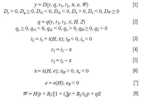
y = output; q = real equity prices; rS = expected short term real interest rate; rL = expected long term rate; π = expected inflation; e = nominal exchange rate (foreign currency per dollar); W = wealth; π = high powered money; Bs = nominal supply of short-term bonds; BL = nominal supply of long-term bonds; p = price level; Z = financial investor confidence, and E = stock of equity in issue. Assumed signs of partial derivatives are indicated by the inequalities.
Equation [1] is the IS schedule in which output is equal to aggregate demand, D. Aggregate demand is a positive function of income, equity prices, expected inflation, and wealth. It is a negative function of the short-and long-term real interest rate, and a negative function of the nominal exchange rate.
Equation [2] determines equity prices as a positive function of income, expected inflation, high powered money, and investor confidence. Equity prices are a negative function of short- and long-term real interest rates. Equation [2] performs the role of the LM schedule in the conventional IS-LM model, capturing income –equity price combinations consistent with equity market equilibrium. In the graphical representation of the model it is denoted the QQ schedule.
Equation [3] is a nominal term structure equation. The slope of the term structure (i.e. the gap between the short- and long-term nominal interest rate) is a negative function of the high powered money supply reflecting a liquidity effect, and a positive function of expected inflation. Equations [4] and [5] define the short- and long-term interest rates.
Equation [6] determines expected inflation which is a positive function of the stock of high powered money and a negative function of the nominal exchange rate. The nominal exchange rate's impact reflects the imported inflation channel.
Equation [6] represents financial market participants' view of inflation and market participants hold monetarist beliefs. It is different from the normal formulation which is usually constructed in terms of some demand pressure variable. This is a critical feature of the model. An economic model represents the way an economist thinks the world works. The model should therefore take account of the way people think, which can be different from the way economists think (Palley 1993). One of the great failures of modern macroeconomics is the assumption of a single true model held by all which ignores this difference.
Equation [7] determines the nominal exchange rate as a negative function of high powered money and expected inflation. Part of an increase in liquidity is directed to foreign currency purchases, causing exchange rate depreciation.
Lastly, equation [8] defines wealth as the real value of the stock market, the stock of high powered money, the stock of short-term bonds, and the stock of long-term bonds. Short-term bonds have a one period maturity and long-term bonds are perpetuities.
Figure 1 provides a graphical analogue of the model. Both the IS and QQ schedules are positively sloped, with the IS assumed to be steeper than the QQ schedule.1 The logic behind the positive IS slope is that aggregate demand is a positive function of equity prices. The logic behind the positive QQ slope is that equity prices are a positive function of income. A sense of the model is provided by considering a positive shock to financial investor confidence. This shifts the QQ schedule up, raising both equity prices and output.

QE IN THE ISQQ MODEL
The zero bound and quantitative easing can be described by setting iS = 0 and adding a policy equation given by either of:
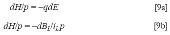
Equation [9a] has quantitative easing implemented via equity purchases, and equation [9b] has it implemented via long-term bond purchases. Note that at the zero bound money and short-term bonds have become perfect substitutes since nominal short-term interest rate is zero. In reality, the fact that there is some liquidity loss to holding short-term bonds means the floor to the nominal short-term interest rate will be fractionally above zero.
Belief in the efficacy of quantitative easing involves the following assumptions:
1. A positive q effect on demand (DqqH > 0).
2. A fall in the long-term real interest rate that stimulates demand (DrLrL,H > 0). This in turn implies the long term nominal bond rate falls by more than expected inflation rises (rL,H = iL,H+ iL,π [πH + πe eH] –πH–πe eH< 0).
3. There is positive expected inflation effect on aggregate demand (Dπ πH> 0).
4. There is a positive exchange rate effect on demand (DeeH > 0).
5. There is a positive consumption wealth effect (DWWH > 0).
The effects of quantitative easing, given these assumptions, are shown in figure 2. The increase in high powered money shifts the QQ schedule up by lowering the expected long-term real interest rate and by increasing expected inflation. It also shifts the IS right by lowering the expected long-term real interest rate, increasing expected inflation, and depreciating the exchange rate.2 The net result is both stock prices and output increase.

WEAKNESSES OF QE
It is now time to turn to the weaknesses of QE that motivate a Keynesian critique. The first weakness is that in deep recession some of the channels of QE may be blocked. One Keynesian argument with a long history is that in deep slumps aggregate demand is insensitive to interest rates. In the original IS-LM model this situation corresponded to a vertical IS schedule. In the current ISQQ model this type of effect is produced if aggregate demand is insensitive to stock prices and the expected short- and long-term real interest rate (Dq = DrL = 0). In this event the IS schedule is steeper as the effect of stock prices is restricted to the wealth effect, and QE only shifts the IS through the expenditure acceleration and exchange rate effects. These QE effects still shift the IS right but the shift is smaller, and the increase in income and stock prices is reduced because the IS is steeper so that induced stock price increases have a smaller positive impact on aggregate demand.
A second more pessimistic scenario is if the IS is sensitive to the expected long-term real interest rate and the real interest rate rises in response to QE. Such an outcome can occur if the long-term nominal interest rate rises by more than expected inflation, which requires the following condition:

A rise in the expected long-term real interest rate has two negative effects on the IS schedule. First, it directly reduces aggregate demand. Second, it negatively affects bond wealth. With regard to the QQ schedule, it decreases the demand for stocks by making long-term bonds relatively more attractive, and it also has a negative wealth effect on the demand for stocks.
The net result is the direction of shift of the IS and QQ schedules is ambiguous. If the positive effects of QE still dominate the IS shifts right and the QQ shifts up, as in figure 2. Figure 3 shows the case where the IS shifts left but the QQ rises because the expected inflation effect on stock demand dominates. In this case, output falls but stock prices rise. A more pessimistic case would have the IS shift left and the QQ schedule shift down. In this event both output and stock prices would fall.

Why might this be so? Here, the beliefs of the bond market and the special conditions associated with the zero bound come in to play. Prior to QE there may have been a bubble in the bond market, with money rushing in to bonds in search of safety. That bubble was working to the Federal Reserve's advantage by driving down the expected long-term real interest rate. In effect, the bond bubble was compensating for being stuck at the zero bound. By undertaking a second round of QE the Fed may have punctured that bubble. Such a situation corresponds to iH >0. When policymakers burst a bond bubble by pushing it too far the signs of partial derivatives may be perverse. This possibility reveals an important consideration for the conduct of monetary policy. Policy should not only take account of how and what the market thinks (which may be very different from the how and what the central bank's economists think via their models), it should also take account of the current speculative condition of markets.
Puncturing a bond bubble is one reason why the real long-term bond rate could rise. A second reason is an overshooting effect of the type identified by Dornbusch (1976). Market participants expect future capital losses on long bond holdings because of higher future inflation. To compensate for those future losses the long-term real bond rate must rise and overshoot now.
A third negative effect concerns commodity price jumps and demand destruction. In this regard, there has been much chatter in financial press about how quantitative easing has flooded the market with liquidity and raised inflation expectations, and that liquidity has in turn sought protection against inflation by buying hard assets in the form of commodities.
Capturing demand destruction effects requires expanding the model to include price level determination and the effect of prices on demand. This introduces Kaleckian effects concerning real wages and income distribution. The price level and income distribution are determined as follows:

p = goods prices; m = firms' mark-up over average cost; w = nominal wage, α = units of commodity input per unit of labor; c = price of commodities; sP = profit share; sW = wage share, and sC = commodity producers' share.
Equation [10] is a mark-up pricing equation in which prices are marked-up over labor and commodity costs per unit of output. Equation [11] is the income shares adding-up constraint. Equation [12] determines the profit share. Equation [13] determines the wage and commodity share. Equation[14] determines the wage share. Equation [15] determines commodity prices as a positive function of market liquidity and expected inflation, and a negative function of the exchange rate. Dollar exchange rate depreciation increases commodity prices indirectly via the expected inflation effect, and directly because it increases global commodity demand by making dollar priced commodities cheaper in the rest of the world. This commodity price exchange rate effect offsets the positive demand-side effect and links to the literature on contractionary devaluation (Krugman and Taylor 1978).
On the demand side the model is expanded to include the effect of real wages and income shares as follows:

The economy is assumed to be wage-led so that an increase in the real wage and wage share both increase demand.3 An increase in the commodity share decreases demand. An increase in the profit share can increase demand if it comes at the expense of commodities, but it reduces demand if it comes at the expense of wages. Commodity producers can be identified with OPEC. An increase in commodity prices is equivalent to a tax on wages and a redistribution of domestic income that lowers aggregate demand. If the commodity price effect is sufficiently strong the IS shifts left in response to QE, as in figure 3. If the effect is strong enough both stock prices and output can fall.
Furthermore, higher product prices will have a negative wealth effect on money, short-term bonds, and long-term bonds. This effect will reinforce the negative real wage and income distribution effect on the IS curve. There will also be a negative wealth effect on stock prices that acts to push the QQ schedule down. Thus again, not only may income fall as a result of QE, but stock prices can fall too.
In the above analysis the mark-up (m) was taken as unaffected by commodity prices. If producers are unable to pass on higher commodity costs to consumers, adverse macroeconomic commodity price effects may lower the mark-up giving rise to profit share complications that affect both stock prices and the goods market.
This possibility can be captured by making the mark-up a negative function of commodity prices and by re-specifying equation [2] so that equity prices are a positive function of the mark-up via the profit share as follows:

In this case, in addition to impacting the goods market, commodity prices also directly affect asset markets. Higher commodity prices have a direct negative effect on equity prices operating via a lower mark-up and industrial profit share. That effect reduces the upward shift of the QQ schedule and could even cause the QQ schedule to shift down. The net result is it is easy to envisage circumstances where QE induced commodity price effects lower both equity prices and output.4
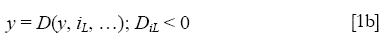
A fourth negative effect of QE concerns long term nominal interest rates. Equation [1] has aggregate demand depend exclusively on expected real interest rates as is the convention in macroeconomics. However, the level of nominal interest rates may also affect aggregate demand so that the IS becomes
The logic of this nominal interest rate effect can be understood by considering the cash flow payments associated with a long term loan with a balloon payment of L to be paid in period T. The stream of real payments (S) is given by

The effect of inflation is to diminish the real value of the balloon repayment. In a period of inflation the nominal interest rate must therefore rise to compensate for this lost purchasing power of loan principal.
Analytically, by causing nominal rates to rise to compensate for the erosion of purchasing power of loan principal, inflation effectively forces an early repayment of the loan. In a world of perfect capital markets this would be of no consequence as borrowers could borrow the early repayment. However, in a world of imperfect capital markets this can introduce cash flow constraints that reduce aggregate demand. This is why the nominal interest rate should be included as an argument in the aggregate demand function.
In terms of the ISQQ model, the nominal interest rate effect of higher expected inflation introduces another channel whereby QE can cause the IS to shift left, as in figure 3. This negative nominal interest rate effect introduces a further channel for QE to have negative impacts and it is likely to be particularly relevant regarding residential mortgages and consumption spending.
In sum, a simple Keynesian styled ISQQ model shows at the theoretical level that there are several channels whereby QE can have negative aggregate demand effects. These include higher long term real interest rates from reversing bond market psychology; higher commodity prices that lower real wages and adversely impact income distribution; adverse wealth effects from higher commodity prices and higher nominal interest rates; and adverse cash flow effects from higher nominal interest rates.
Despite this, the Federal Reserve (Bernanke 2011) has unilaterally asserted that its second round of QE has been an unequivocal success. The Fed's claim is empirically dubious as it is widely agreed that monetary policy is characterized by long and variable lags and not enough time has gone by to detect meaningful effects. The above model shows it is also theoretically dubious. Moreover, commodity prices and interest rates have actually responded to the Federal Reserve's second round of QE in a manner consistent with these negative theoretical effects.
FURTHER CRITIQUES OF QE
The ISQQ model illuminates the most immediate macroeconomic channels whereby QE may backfire. In addition to these channels there are a number of other concerns not in the model.
A first downside is the possibility of QE creating another price bubble in "hard" assets that causes significant wealth destruction when it bursts later. People need to save, especially in light of the shift from defined benefit to defined contribution pension plans. Since QE depresses yields, especially on traditional shorter-term saving instruments, households are encouraged to engage in a chase for yield to preserve income. However, that exposes them to large capital losses later. The implication is that by facilitating bubbles, QE makes planning for the future more difficult and risks imposing arbitrary outcomes that produce highly undesirable household welfare effects. By artificially pumping up asset prices, QE exposes asset prices to subsequent falls. The generalized psychological damage of those falls can easily outweigh the small benefit of any wealth effects on demand.
In addition to adverse household welfare effects, sponsoring bubbles can also cause systemic financial fragility as banks, insurance companies and other financial intermediaries are encouraged to take greater risk in their own chase for yield. The cost of such bubbles is two-fold. First, there is the cost of misallocation of capital to unproductive uses. Second, there is the cost of collateral damage inflicted when the bubble bursts. The recent housing bubble and the 1990s Internet stock bubble provide evidence of both types of cost.
A second downside concerns the risks associated with policy volatility. The Federal Reserve has injected enormous liquidity into the financial sector. That liquidity carries two types of risk. The first is it triggers actual inflation that prompts the Fed to raise short-term nominal interest rates abruptly. The second is the Federal Reserve, for reasons of its own policy preferences, raises interest rates abruptly. In either case, the risk is a sudden spike in the short-term policy interest rates could cause significant disruption as happened in 1994. This risk can be understood through the metaphor of a car slamming on the brakes and causing the occupants to fly through the windshield. The damage from slamming on the brakes is inversely related to the speed of the car.
A third concern is adverse international effects. QE is likely to depreciate the exchange rate as domestic wealth holders use liquidity to buy foreign assets. As noted above, on one hand that stands to benefit the U.S. economy by changing the relative price of exports and imports. Balanced against that, it can worsen commodity price jump effects. Another problem in the current environment is the wrong currencies may do the appreciating. Thus, the U.S. trade deficit problem is essentially with China, but China's exchange rate is controlled. Consequently, dollar depreciation may take place against Brazil and Europe which are both playing by the rules of the game. In doing so, QE may add to international economic tensions and destabilize the global economy to the extent it punishes the innocent.
In sum, concerns with potential for bubbles, future costs of reversing QE, and the possibility for undesirable international effects add to the macroeconomic downsides of QE identified by the ISQQ model.
PLUTONOMICS AND THE POLITICAL ECONOMY OF QE
A third and final line of argument against QE concerns its embedded political economy. In many respects the Federal Reserve finds itself in a position similar to that of 2001-2003, only worse. Back then the economy was stuck in jobless recovery and the Federal Reserve was unable to jump start recovery, prompting its turn to extended ultra-easy monetary policy. Today, the economy is in an even worse position of jobless recovery because the slump has been deeper and household balance sheets have been ravaged by the house price collapse and debt accumulated during the house price bubble.
The underlying problem is structurally deficient demand caused by thirty years of neoliberal economic policies that have undermined the income and demand generation process (Palley 2009). However, rather than fixing this problem, policymakers are again turning to ultra-easy monetary policy in the form of QE.
Viewed from this perspective, QE can be interpreted as a form of asset market trickledown whereby supporting asset prices is supposed to jumpstart the macro economy. Under Chairman Greenspan the Federal Reserve put in place an asset price floor, widely referred to as the "Greenspan put": the Fed would intervene to support asset prices any time a deep fall threatened. Under Chairman Bernanke this policy has evolved into an asset price subsidy in the form of QE. The Fed will now intervene to actively bid up asset prices to jump start the economy.
From a political standpoint, this is an enormous change from the world of forty years ago. The New Deal policy paradigm of wage floors and household income supports has been replaced by one of asset price floors and asset market subsidies. Viewed through a political lens QE therefore represents the triumph of plutonomics, and that makes it an obstruction to the extent it obscures the challenge of repairing the income and demand generation process.
CONCLUSION: RETHINKING KEYNESIAN SUPPORT FOR QE
Economists of Keynesian persuasion have generally been quick to embrace QE on the grounds that it increases aggregate demand and anything that increases demand at this time of demand shortage is welcome. This paper has argued that reaction may be misplaced. QE holds dangers of backfiring with respect to demand stimulus, carries potentially significant future costs and dangers, and is supportive of a plutocratic political economy that obstructs needed policy change.
New classical economists reject QE on the grounds that unemployment is of the structural mismatch type and easy monetary policy cannot fix such unemployment and only risks inflation. Keynesians reject the unemployment mismatch argument because all regions and sectors of the labor market have experienced increased unemployment and there is no evidence of significant sector specific excess demand and rising wages (De Long 2010).
However, there is a different Keynesian structural argument for rejecting QE. That argument is there are structural problems on the demand side of the economy concerning the income and demand generating process. Those problems concern income distribution and they cannot be fixed via monetary policy.
This Keynesian argument against QE can be thought of in terms of second-best theory (Lancaster and Lipsey 1956). If policymakers were to seriously address the problems of the income and demand generation process, QE might be useful in facilitating the transition to a new system. However, pursuing QE alone without addressing the demand side structural problems may actually harm the economy. That fits with the logic of second best theory in which fixing one market imperfection in the presence of many can actually worsen outcomes.
Finally, another perspective on QE comes from monetary macroeconomics which argues that monetary ease in a deep recession is like "pushing on a string". There should be a corollary proposition that monetary authorities should not let out too much string in case they create a knot, which is what QE risks doing.
REFERENCES
Bernanke, B.S.; V.R. Reinhart and B.P. Sack, "Monetary policy alternatives at the zero bound: an empirical assessment", Divisions of Research & Statistics and Monetary Affairs, Federal Reserve Board, Finance and Economics Discussion Series no.48, 2004. [ Links ]
Bernanke, B.S., "The economic outlook and monetary policy", Speech at the National Press Club, Washington, D.C., February 3, 2011. [ Links ]
De Long, J.B., "The price of inaction", Project Syndicate, April 28, 2009. Available at: <http://www.project-syndicate.org/commentary/delong89/English> [ Links ].
––––––––––, "The varieties of unemployment", Project Syndicate, August 31, 2010. Available at: <http://www.project-syndicate.org/commentary/delong105/English> [ Links ].
Dornbusch, R., "Expectations and exchange rate dynamics", Journal of Political Economy, no. 84, 1976, pp. 1161-1176. [ Links ]
Farmer, R., "A new monetary policy for the 21st century", FT.com/Economists' Forum, January 12, 2009. Available at: <http://blogs.ft.com/economistsforum/ 2009/01/a-new-monetary-policy-for-the-21st-century/> [ Links ].
Krugman, P., "Bernanke and the Shibboleths", Conscience of a Liberal Blog, November 6, 2010. Available at: <http://krugman.blogs.nytimes.com/2010/11/06/bernanke-and-the-shibboleths/> [ Links ].
Krugman, P. and L. Taylor, "Contractionary Effects of Devaluation", Journal of International Economics, 1978, no. 8, pp. 445-456. [ Links ]
Lancaster, K. and R.G. Lipsey, "The general theory of the second-best", Review of Economic Studies, vol. 24(1), 1956, pp. 11-32. [ Links ]
Meltzer, A.H., "Ben Bernanke's '70s show", Wall Street Journal, February 5, 2011. [ Links ]
Neary, J.P. and J.E. Stiglitz, "Towards a reconstruction of Keynesian economics: expectations and constrained equilibria", Quarterly Journal of Economics, no. 98, Supplement, 1983, pp. 196-201. [ Links ]
Palley, T.I., "Uncertainty, expectations, and the future: if we don't know the Answers, what are the Questions?", Journal of Post Keynesian Economics, 1993, pp. 1-20. [ Links ]
––––––––––, "America's exhausted paradigm: macroeconomic causes of the financial crisis and great recession", New American Contract Policy Paper, New America Foundation, Washington, D.C. July 22, 2009. Available at: <http://www.newamerica.net/publications/policy/america_s_exhausted_paradigm_ macroeconomic_causes_financial_crisis_and_great_recession> [ Links ].
––––––––––, "Inside debt and the stability of inflation", Eastern Economic Journal, forthcoming, 2011. [ Links ]
Taylor, J.B., "A two-track plan to restore growth", Wall Street Journal, January 28, 2011. [ Links ]
Tobin, J. and W. Buiter, "Fiscal and monetary policies, capital formation, and economic policy," in von Furstenberg (ed.), The Government and Capital Formation, Ballinger Publishing, 1980, p. 73-151. [ Links ]
* This paper was presented at the Eastern Economic Association meetings held in New York, NY, February 25-27, 2011. I thank meeting participants for their useful comments. All errors and omissions are mine.
** JEL: Journal of Economic Literature–Econlit.
1 A simple phase diagram analysis using the adjustment equations Δy/y = f(D – y), f '> 0, f(0) = 0 and Δq/q = g(q – q *), g'< 0, g(0) = 0 shows this pattern is needed to ensure stability.
2 Note, the impact of the Tobin q effect and the effect of stock prices on wealth are built into the slopes of the IS and QQ schedules.
3 The relationship between the wage share and profit share depends on whether the economy is wage-led or profit-led. In a wage-led economy increasing the wage share at the expense of the profit share increases demand and output, the assumption being the increase in consumption exceeds any decrease in investment. A profit-led economy is characterized by the reverse.
4 Having commodity prices affect the mark-up and profit share would also introduce additional impacts on the IS. On the negative side, it would adversely impact the IS by reducing the consumption wealth effect that comes from increased wealth due to QE. On the positive side, the fact that profits bear part of the brunt of higher commodity prices means that real wages and the wage share do not fall as much.

