


Servicios Personalizados
Revista
Articulo
 Inglés (pdf)
 Artículo en XML
 Referencias del artículo
 Enviar artículo por email
Indicadores
-
 Citado por SciELO
 -
 Accesos
Links relacionados
-
 Similares en
SciELO
Similares en
SciELO
Compartir

 Permalink
Investigación económica
versión impresa ISSN 0185-1667
Inv. Econ vol.68 no.270 Ciudad de México oct./dic. 2009
The backward bending Phillips curves: competing micro–foundations and the role of conflict
La curva de Phillips invertida: microfundamentos rivales y el papel del conflicto
Thomas I. Palley
New America Foundation, mail@thomaspalley.com
Received June 2009
Accepted September 2009
Abstract
This paper excavates the micro–foundations of the Phillips curve and presents a model of the backward bending Phillips curve that incorporates elements of wage conflict. This unifies the conflict and demand–pull approaches that are often viewed as separate. There are two alternative micro–foundations for the Phillips curve. One emphasizes worker–firm conflict and incorporation of inflation expectations into nominal wages: the other emphasizes behavioral economics and near–rationality of expectations. A Phillips curve can emerge either because workers systematically under–predict inflation via near–rationality, or because workers do not fully incorporate inflation expectations owing to local unemployment conditions that induce wage concessions.
Key words: backward bending Phillips curve, behavioral economics, conflict economics.
Classification JEL:* E00, E31, E52
Resumen
Este trabajo analiza los micro–fundamentos de la curva de Phillips y presenta un modelo de la curva Phillips invertida que incorpora elementos de conflicto salarial. El modelo considera conjuntamente los dos enfoques de la curva de Phillips, el de conflicto y el de demanda, que frecuentemente se tratan de manera separada. Existen dos micro–fundamentos alternativos para la curva de Phillips. El primero enfatiza el conflicto entre trabajadores y empresas y la incorporación de las expectativas de inflación en los salarios nominales; el segundo, enfatiza la economía del comportamiento y la cuasi–racionalidad de las expectativas. La curva de Phillip s puede emerger sea porque los trabajadores subestiman sistemáticamente la inflación a través de cuasi racionalidad o porque no incorporan las expectativas de inflación completamente debido a condiciones de desempleo locales que inducen concesiones salariales.
Palabras clave: curva de Phillips invertida, economía del comportamiento, economía del conflicto.
THE PHILLIPS CURVE AND MACROECONOMICS
The Phillips curve is a critical part of macroeconomics, yet the theoretical foundations of this important relation remain poorly understood. The current paper excavates the micro–foundations of Phillips curve theory, focusing on the competing theoretical explanations of the Phillips curve that adopt a demand–pull perspective.
The paper develops a taxonomy of the different theoretical approaches to the Phillips curve, and then presents a simple model of the backward bending Phillips curve that incorporates elements of wage conflict. The model therefore joins together the logic of both the conflict and demand–pull approaches to the Phillips curve, which in the past have been kept separate.
A TAXONOMY OF THE PHILLIPS CURVE
Macro models usually include the Phillips curve as a structural equation that determines the rate of inflation as a function of capacity utilization or the unemployment rate. From a policy perspective, it is a critical constraint because economic outcomes are ultimately constrained to lie on the Phillips curve.
Figure 1 provides a taxonomy of the Phillips curve. There are two broad approaches: the empirical approach and the theoretical approach. The origins of the Phillips curve are empirical and based on Phillips' (1958) seminal paper. Significant contributors in this extensive tradition include Robert Gordon (1983) and Robert Eisner (1997). However, as Tobin (1972) observed, "The Phillips curve is an empirical finding in search of a theory, like Pirandello characters in search of an author (1972, re–printed 1975:45)." That means an empirical approach can document the existence and shape of the Phillips curve and suggest variables that might be theoretically relevant, but there is also need for theoretical explanation of this empirical relation (i.e. why do economies generate data patterns like the Phillips curve).

In figure 1 the theoretical approach is divided into the conflict approach and demand–pull approach. The conflict approach is emphasized by Post Keynesians (Myatt 1986; Dalziel 1991; Lavoie 1992; Palley 1996) and it represents inflation as the product of inconsistent claims on national income by capital and labor. The demand–pull approach has tended to be emphasized by neo–Keynesians, new classicals, and new Keynesians. In that story, inflation is determined by inflation expectations and the state of excess demand in the labor or goods market. The two approaches have been segmented, and one purpose of the current paper is to establish some commonalities by showing how labor market conflict also plays a role in the demand–pull approach.
The demand–pull approach is itself divided into the neo–classical approach associated with Lipsey (1960), Friedman (1968), and Phelps (1968), and the dynamic stochastic disequilibrium approach of Tobin (1972). The neo–classical approach assumes an aggregate labor market, and it views the Phillips curve and inflation as the product of gradual disequilibrium adjustment in a conventional neo–classical aggregate labor market. The problem with this approach is that it is hard to generate a negatively sloped long–run Phillips curve.1
The Tobin dynamic stochastic disequilibrium approach uses a multi–sector framework in which there are multiple segmented labor markets. That makes it intrinsically more difficult to model, which has hindered its dissemination —especially in textbooks—. The significance of the multi–sector approach is that the economy can simultaneously have conditions of excess demand in some labor markets and excess supply in other labor markets. As discussed below, that pattern enables inflation to help economic adjustment in a particular way.
In the neo–classical single labor market model excess demand raises inflation and faster inflation helps restore equilibrium by reducing excess demand. However, once excess demand is eliminated and supply–demand balance is re–established, inflation falls back and has no further real impact on the labor market.
Tobin dynamic stochastic disequilibrium approach is fundamentally different. Aggregate nominal demand growth causes inflation in sectors at full employment but helps reduce unemployment in sectors with unemployment. That pattern effectively generates a Phillips curve, defined as a negative correlation between inflation and unemployment. This type of outcome is not possible in a single market model in which the economy either has excess demand or has excess supply. Furthermore, as long as economies are marked by the presence of persistently recurring sector disequilibria (due to stochastic sector demand shocks), steady nominal demand growth that produces inflation can have a permanent role in reducing disequilibrium unemployment caused by on–going recurring sector demand shocks.
MICRO–FOUNDATIONS OF THE TOBIN APPROACH TO THE PHILLIPS CURVE
The Tobin approach to the Phillips curve has itself spawned a separate subset of models, as illustrated in figure 2. Earlier models based on the Tobin approach sought to derive the conventional long–run negatively sloped Phillips curve (Palley 1994, 1997; Akerlof et al. 1996). More recent models have argued for a backward bending Phillips curve that is negatively sloped at low rates of inflation, but becomes positively sloped and then vertical as the inflation rate increases (Akerlof et al. 2000; Palley 2003).

The critical features of the Tobin model are (1) its multi–sector framework that allows the co–existence of excess labor demand and supply, and (2) downward nominal wage rigidity. This downward nominal wage rigidity prevents labor markets with excess supply from adjusting, which is why creating aggregate excess demand can help "grease" the adjustment process. It does so by causing inflation in sectors at full employment while creating employment in sectors with unemployment.2
A key theoretical assumption of the Tobin model is that the process of nominal wage adjustment is different in sector labor markets with full employment nominal wages are perfectly flexible and are bid up to their market clearing level. However, in sectors with unemployment nominal wage adjustment is downwardly rigid.
With regard to nominal wage adjustment in sectors with unemployment, there are two distinct aspects. The first concerns how nominal wages respond to disequilibrium unemployment. The second concerns how nominal wages respond to persistent inflation —i.e. the inflation expectations component—. Explaining this nominal wage setting behavior provides the link between Tobin's multi–sector demand–pull Phillips curve and Post Keynesian conflict inflation.
One approach to explaining nominal wage adjustment in sectors with unemployment is via behavioral economics. This behavioral approach has been used by Akerlof et al. (1996, 2000) and involves the following two assumptions:
A.1. Nominal wages are downwardly rigid because of worker concerns with relative wages. Workers in sectors with unemployment therefore resist wage reductions because of resistance to taking a wage cut relative to workers in sectors with full employment (Akerlof et al. 1996).
A.2. With regard to inflation, nominal wages increase less than expected inflation because workers have money illusion arising from near–rationality. At low rates of inflation workers either overlook the effects of inflation or take them into account less than fully. However, at some threshold rate of inflation workers start taking full account of inflation, and this generates a backward bending Phillips curve (Akerlof et al. 2000; Rowthorn 1977).
An alternative labor market microeconomics in the spirit of Post Keynesian conflict theory is suggested by Palley (1990, 1994, 1997, 2003). This conflict microeconomics also explains the existence of the Phillips curve and it involves the following assumptions:
B.1. Labor exchange is characterized by conflict and moral hazard. Workers in sectors with unemployment therefore resist wage reductions imposed from within the employment relationship for fear that firms are trying to cheat them. However, workers are willing to accept some real wage reduction imposed from outside the employment relationship via inflation that raises the general price level. That is because the general price level is outside the control of individual firms so workers know their firm is not opportunistically taking advantage of them (Palley 1990, 1994, 1997).3
B.2. However, though willing to accept some real wage reduction via price inflation, workers resist excessive real wage reductions imposed by unacceptably high inflation. Thus, as inflation increases, more and more workers in sectors with unemployment start demanding nominal wage increases that match inflation in order to protect their real wage (Palley 2003).
When such conflictive nominal wage setting behavior is placed in a multisector economy in which some sectors have unemployment and others are at full employment, it too can generate a backward bending Phillips curve. The logic is as follows. Initially, nominal demand growth causes inflation in full employment sectors, and creates jobs in sectors with unemployment where nominal wages remain fixed. Faster nominal demand growth generates faster inflation in full employment sectors and more employment creation in sectors with unemployment. However, some workers in sectors with modest unemployment start indexing their wages, thereby partially reducing the grease effect of nominal demand growth in those sectors. The grease effect is reduced because nominal wages in those sectors start matching inflation, thereby neutralizing the job creation impact of nominal demand growth.4
As inflation increases, workers in more and more sectors with unemployment start resisting real wage reductions, progressively eroding the grease effect. At some stage the Phillips curve bends back because adding more grease (nominal demand growth that causes inflation) is outweighed by decreased lubricity (indexing of nominal wages to inflation). Eventually inflation is pushed to a high enough level that all workers are indexing, and the Phillips curve becomes vertical.
Table 1 provides a summary of the micro–foundations involved in constructing Tobin–d Phillips curves. There are two alternative micro–foundations for nominal wage setting: behavioral microeconomics or conflictive microeconomics. Both can generate a standard negatively sloped Phillips curve or a backward bending Phillips curve.

Behavioral microeconomics generates a standard Phillips curve with assumption A.1 (Akerlof et al. 1996). It generates a backward bending Phillips curve with assumptions A.1 and A.2 (Akerlof etal. 2000; Rowthorn 1977). Conflictive microeconomics generates a standard Phillips curve with assumption B.1 (Palley 1994, 1997). It generates a backward bending Phillips curve with assumptions B.1 and B.2 (Palley 2003).
INFLATION, LABOR MILITANCY, AND THE BACKWARD BENDING PHILLIPS CURVE
This section presents a new model of the backward bending long run Phillips that explicitly highlights why inflation is associated with lower unemployment rates in a multi–sector economy. The model captures the economic logic in the backward bending Phillips curve developed in Palley (2003). It also highlights the role of labor market militancy, which is defined as the sensitivity of nominal wage demands of workers in sectors with unemployment to inflation. As workers become more militant the Phillips curve steepens quicker and bends back at a higher rate of unemployment. In effect, the Friedman (1968)–Phelps (1968) assumption that all workers (including those in sectors with unemployment) fully incorporate inflation expectations into their nominal wage demands corresponds to the assumption of maximum worker militancy.
The model is given by the following four equations:
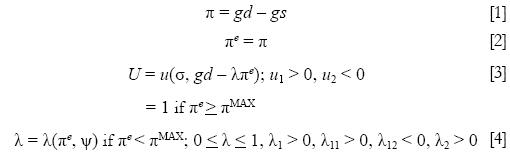
where π = inflation rate, πe = expected inflation rate, πMAX = critical inflation rate at which all workers fully index nominal wages, gd = growth of nominal demand, gs = productivity growth, U= unemployment rate, σ = dispersion of sector specific nominal demand shocks that have a mean of zero, λ = aggregate coefficient of inflation expectations, and ψ = worker militancy variable affecting the degree of real wage resistance.
Equation [1] describes the economy's inflation generating process. The long run equilibrium inflation is equal to the rate of aggregate nominal demand growth minus the rate of productivity growth. Henceforth, for simplicity, it is assumed that gs = 0.
Equation [2] has expected inflation equal to actual inflation. That means any inflation–unemployment trade–off that exists is not due to misperceptions.
Equation [3] describes the economy's long run unemployment rate generating process. The first argument in the function u(.) has unemployment depending positively on the dispersion of nominal demand shocks across sectors.5 Each period sectors receive nominal demand shocks that sum to zero (i.e. some sectors receive positive shocks, others receive negative shocks). These shocks give rise to frictional unemployment that is located in sectors receiving negative demand shocks. The greater the dispersion of these shocks, the greater will be the extent of frictional unemployment at any moment in time.
The second argument captures the nominal demand growth grease effect. This effect on unemployment results from nominal demand growth that creates jobs in sectors with unemployment. The extent to which nominal demand growth creates jobs depends on the extent to which it is offset by nominal wage increases in sectors with unemployment. If workers show nominal wage restraint (low λ), then nominal demand growth will have a large job impact. However, if workers are militant and raise nominal wages to compensate for inflation (high λ), then nominal demand growth will be offset by inflation and yield little job creation.
Equation [4] describes the determination of the aggregate coefficient of inflation expectations. This coefficient captures the extent of real wage resistance to inflation. There are two regimes: the high inflation regime and the low inflation regime. In the high inflation regime the aggregate coefficient of inflation expectations is unity. That is because inflation is at or above πMAX so that all workers in all sectors fully index their nominal wages. In the low inflation regime inflation is below πMAX so that only some workers fully index and the aggregate average coefficient of inflation expectations is less than unity. As inflation increases, more and more workers fully index so that the coefficient and the extent of real wage resistance increase.
The economic logic of the model is described in figure 3. The underlying economic driver is the rate of aggregate nominal demand growth that simultaneously increases the rate of inflation by causing inflation in sectors at full employment, and lowers the rate of unemployment by creating jobs in sectors with unemployment. The economics literature (see for instance Card and Hyslop 1997; Groshen and Schweitzer 1997) commonly refers to "inflation's grease effect" on labor market adjustment and unemployment. That characterization is wrong. The reality is nominal demand growth is the grease, and higher inflation and lower unemployment are the products of faster nominal demand growth.
The economic logic represented in figure 3 reveals that the long run Phillips curve is a locus of points in inflation–unemployment rate space rather than a causal relation. This locus emerges because nominal demand growth generates a negative correlation between inflation and unemployment. That correlation is due to a common factor, which is nominal demand growth. This contrasts with standard macroeconomic representations of the demandpull Phillips curve that they make it look as if there is a causal long–run relationship between inflation and unemployment. That is not the case.

The coefficient of real wage resistance, λ is critical. As can be seen from equation [3], if the coefficient is unity, unemployment is unaffected by nominal demand growth and unrelated to inflation. The aggregate coefficient of real wage resistance is a weighted average of the sector real wage resistance coefficients. In sectors with full employment λ = 1, but in sectors below full employment it may be less than unity at lower levels of inflation —which is why the aggregate average can also be less than unity—. As aggregate unemployment increases λ will tend to fall as fewer sectors are at full employment. The reverse holds when aggregate unemployment decreases.6
The idea that nominal demand growth greases labor market adjustment can be understood as follows. Let z denote the magnitude of the grease effect —the coefficient of lubricosity—. This coefficient is equal to the gap between aggregate nominal demand growth and the feedback of inflation into nominal wage setting, and it is given by

Using the assumption gs = 0, equations [1]–[4] imply the grease effect is

If gd is positive, this grease effect is always non–negative since 0 ≤ λ, ≤ 1. If gd= 0 then z = 0. Likewise, if λ = 1 then z = 0. Differentiating z with respect to gd yields

Thus, increases in nominal demand growth can increase the grease effect or decrease it.7 When gd and inflation are low both of the negative terms (λ + λ1gd) will be small and increases in gd will raise the grease effect. When gd is large and inflation is high the reverse holds.
The evolution of z as a function of gd is shown in figure 4 and z reaches a maximum when gd = gd* = [1 – λ]\ λ1. The logic is as follows. At low inflation, faster nominal demand growth adds to real demand growth because price and wage inflation is held down in sectors with high unemployment because workers show nominal wage restraint. However, as inflation rises, wage restraint is progressively abandoned which takes back some of the grease effect, and hence the hump shape.

The effect of faster nominal demand growth and inflation on unemployment is given by

When the grease effect is positive (i.e. at low inflation), the unemployment rate falls in response to faster nominal demand growth and inflation. Once the grease effect has peaked, faster nominal demand growth and inflation raise the unemployment rate. This corresponds to being on the backward bending part of the Phillips curve. The backward bending inflection point occurs when z is at a maximum, which occurs when gd* = [1 – λ]\λ1.
The vertical portion of the Phillips curve corresponds to the high inflation regime and has λ = 1. Consequently, faster nominal demand growth and inflation have no effect on unemployment. The unemployment rate is given by u = u(σ, 0). This is the same unemployment rate that obtains when nominal demand growth and inflation are zero.
Such a backward bending Phillips curve is shown in figure 5. In place of a non–accelerating inflation rate of unemployment (NAIRU) that acts as a constraint on the sustainable minimum unemployment rate, there is a minimum unemployment rate (MUR) that pairs with a minimum unemployment rate of inflation (MURI). The MURI is the inflation rate that obtains at the point of inflexion when the Phillips curve bends backward and the MURI represents the point where the labor market grease effect of nominal demand growth is maximized.

INCORPORATION OF INFLATION EXPECTATIONS VERSUS FORMATION OF INFLATION EXPECTATIONS
The aggregate coefficient of inflation expectations, λ, plays a critical role in the backward bending Phillips curve and it can also be related to both the NAIRU and neo–Keynesian expectations augmented Phillips curve models.
The Friedman (1968) and Phelps (1968) NAIRU model implicitly assumes that λ = 1 so that all the grease effect of nominal demand growth is crowded out by equal proportionate increases in nominal wages and prices.
The conventional neo–Keynesian Phillips curve assumes that λ is a constant lying between zero and unity (Tobin 1971) so that some part of nominal demand growth is not crowded out. However, neo–Keynesians provided no theoretical explanation for this assumption.
Unfortunately, in the 1970s the debate over the Phillips curve was sidetracked into a debate over whether inflation expectations were adaptive or rational. Systematically under–predicting inflation is one way that nominal demand growth can have a persistent effect on unemployment. However, an alternative is that agents rationally predict expected inflation, but do not fully incorporate their inflation expectations into their nominal wage demands. That approach can explain why econometric regressions of the expectations augmented Phillips curve so often report that the coefficient of inflation expectations is less than unity.
This latter explanation was not adopted in part because macroeconomists were working with aggregate models with a single labor market. Consequently, it is difficult to rationalize why the coefficient of inflation expectations would be less than unity when there is inflation and excess demand. However, when the economy is viewed as consisting of multi–sector labor markets rather than a single aggregate labor market, that coefficient is a weighted average of the feed through of inflation expectations across all sectors. It can therefore be less than unity if some sectors are showing wage restraint because of local employment conditions. Workers in those sectors can have fully rational expectations about inflation, but such restraint can be the optimum response given their local concern with jobs.
The issue of "formation" versus "incorporation" of inflation expectations is what distinguishes the backward bending Phillips curve developed by Akerlof et al. (2000) from that developed by Palley (2003). Akerlof et al. (2000) continue to focus on the issue of formation of inflation expectations, replacing rational expectations with near–rational expectations. Palley (2003) focuses on incorporation of inflation expectations.
In the Akerlof et al. (2000) model λ is unity, but workers have near–rational expectations that systematically underestimate inflation when it is low but correctly estimate inflation at higher levels. Since the underestimate is persistent, that preserves the negatively sloped Phillips curve —unlike adaptive expectations in which expectations catch up with actual inflation so that the negatively sloped Phillips curve can only be preserved by accelerating inflation (Friedman 1968).
Equations [1]–[4] describe the backward bending Phillips curve model developed by Palley (2003). The backward bending Phillips curve model developed by Akerlof et al. (2000) model can be understood as follows:

The key differences concern the formation of inflation expectations (equation [2.1]) and the grease effect (equation [4.1]).
Equation [1.1] determines the actual inflation rate. Equation [2.1] determines inflation expectations, which are formed near–rationally. At low inflation rates workers systematically underestimate inflation, but once inflation crosses a threshold of π* they correctly estimate inflation.8 As inflation rises, aggregate average expected inflation converges to actual inflation. Equation [3.1] determines the unemployment rate, while equation [4.1] determines the nominal demand growth grease effect.
Equation [4.1] has full feedback of expected inflation into the nominal wage setting process since λ = 1, but since expectations are near–rational and slightly below actual inflation, this leaves space for nominal demand growth to have a grease effect. However, as inflation increases, near–rationality is progressively abandoned by workers at different firms, thereby eroding the grease effect. When πe = π the grease effect is fully eroded and the Phillips curve becomes vertical, with the unemployment rate equal to the natural rate.
The effect of progressive abandonment of near–rational inflation expectations on the Phillips curve can be formally analyzed as follows. Combining equations [1.1], [2.1] and [4.1] and settinggs = 0, yields a grease effect given by z = gd – πe(gd). Differentiating z with respect to gd yields dz/dgd = 1 – πe1 >< 0 if πe1>< 1. The marginal grease effect can therefore be positive or negative. The Phillips curve is negatively sloped when it is positive and positively sloped when it is negative. Further differentiating z with respect to gd yields δ2z/δgd2 = πe11 < 0 Thus, the marginal grease effect (lubricosity) is strictly declining and the Phillips curve bends back when the marginal effect is zero.
This formulation contrasts with the earlier formulation in equations [1]–[4] that is based on Palley (2003). In that model workers correctly expect inflation (πe = π) and can have fully rational expectations, but they knowingly hold the line on nominal wage increases because of local sector unemployment conditions. Consequently, the aggregate average value of λ is less than unity because of intentional nominal wage setting behavior in sectors with unemployment. In effect, the focus is shifted from formation of inflation expectations to incorporation of inflation into to nominal wage setting via the coefficient of real wage resistance. The grease effect disappears when λ is unity.
WORKER MILITANCY AND THE TOBIN MULTI–SECTOR DEMAND PULL–MODEL
The slope of the backward bending Phillips curve and its turning point depend on how rapidly workers start to display real wage resistance (i.e. how sensitive λ is to πe). If workers start displaying real wage resistance at low inflation rates, the Phillips curve will be steep and also bend back at a relatively low rate of inflation and high rate of unemployment. If real wage resistance only develops slowly, the Phillips curve will be flatter and will bend back at a higher rate of inflation and lower rate of unemployment.
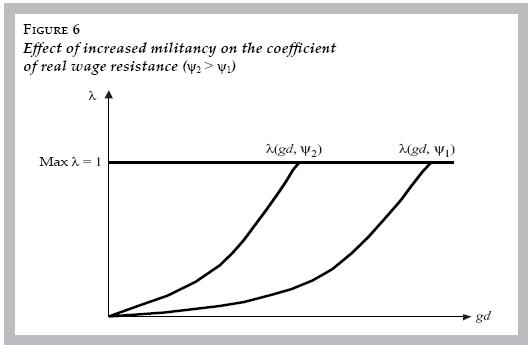
This links the demand–pull model to issues of labor market conflict and worker militancy. Worker militancy can be thought of as a political attitude that influences the behavior of the coefficient of inflation expectations. This militancy effect enters via the parameter ψ in equation [4], and the effect of increased worker militancy on real wage resistance is shown in figure 6. An increase in militancy (ψ2 > ψ1) raises the coefficient of inflation expectations ( λ) for any level of expected inflation. That means nominal wages start to incorporate more of expected inflation.
The effect of increased worker militancy on the Phillips curve operates through militancy's impact on nominal demand growth's grease effect. Differentiating z with respect to ψ yields

Increased militancy therefore decreases the nominal demand grease effect as shown in figure 7.

Weakening of the grease effect in turn causes the Phillips curve to bend back at lower rates of inflation and higher rates of unemployment, and it also causes the Phillips curve to become vertical at lower rates of inflation. These effects of increased militancy are shown in figure 8. The economic logic is as follows. Increased militancy diminishes the grease effect so that unemployment is higher for every rate of inflation. It also causes the grease effect to peak earlier, which causes the Phillips curve to bend back at a lower inflation rate and higher unemployment rate. This can be seen by differentiating gd* with respect to ψ, which yields

gd* is the rate of nominal demand growth and inflation at which the Phillips curve bends back, and increases in worker militancy lower this rate. Finally, the Phillips curve becomes vertical when z = 0, which holds when λ(πe, ψ) 1. Increases in worker militancy raise the value of λ holding gd constant, so that the Phillips curve becomes vertical at lower rates of nominal demand growth and inflation.
FURTHER ANALYTICS
Increases in the dispersion of sector demand shocks (σ) raise the equilibrium rate of unemployment, but have no effect on inflation. This can be seen by differentiating equations [1] and [3] with respect to σ, which yields

Increased dispersion of sector demand shocks can be interpreted as raising frictional and structural unemployment, but they leave equilibrium inflation and the grease effect unchanged. Increased dispersion of sector demand shocks therefore shifts the Phillips curve horizontally as shown in figure 9.

Finally, it is interesting to consider the effect of productivity growth. If productivity growth is non–zero, the rate of inflation and unemployment are given by

Productivity growth therefore lowers inflation for any given rate of nominal demand growth. It also lowers equilibrium unemployment, which can be seen by differentiating [8] with respect to gs

The logic is that faster productivity growth lowers inflation, which lowers nominal wage inflation and allows more job creation in sectors with unemployment from a given rate of nominal demand growth.
POLICY IMPLICATIONS
The backward bending Phillips curve has important theoretical and policy implications. One theoretical implication concerns static modeling of monetary policy which is often thought of as operating through changes in the level of interest rates that in turn impact the level of real aggregate demand. A Phillips curve perspective sees monetary policy as operating through its impact on nominal demand growth. Monetary policy effectively manages nominal demand growth, contingent on the rate of productivity growth, to obtain the desired rate of inflation or unemployment.
This can be represented by the following specification of the policy process:
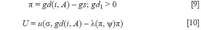
where i = policy interest rate and A = vector of exogenous variabls affecting nominal demand growth. Given an inflation target, the monetary authority solves equation [9] for the interest rate that hits the target. If it has an unemployment target, it solves equation [10] for the interest rate that ensures nominal demand growth appropriate for that target.
An important feature of the backward bending Phillips curve is that it restores a trade–off between inflation and unemployment for low rates of inflation. If the monetary authority is aiming for the lowest possible sustainable rate of unemployment, it should aim for an inflation rate equal to the MURI.
The notion of a MURI has implications for current policy. The Federal Reserve and other central banks commonly focus on an informal inflation target of two percent, but there is little reason to believe that two percent is the MURI. Historical evidence for the United States (U.S.) suggests that the unemployment rate is lowest when inflation has been in the 3–5 percent range. Moreover, Akerlof et al. (2000) present empirical evidence that the Phillips curve may even bend back at around seven percent inflation.
Another policy implication concerns changes in worker militancy and real wage resistance. Decreases in worker militancy lower real wage resistance, causing the Phillips curve to bend back at a lower unemployment rate and higher inflation rate —i.e. they lower the MUR and raise the MURI—. From a policy standpoint, that means that the monetary authority should raise its estimate of MURI, enabling it to push for lower rates of unemployment. This is relevant for the U.S. economy today. Indeed, as long ago as 1999 former Federal Reserve Chairman Alan Greenspan (1999) openly commented about workers' heightened sense of job insecurity tamping down real wages.
Lastly, increases in the underlying rate of productivity growth also allow the monetary authority to step on the economic accelerator. This is because accelerated productivity growth directly lowers inflation, and it also lowers unemployment by lowering inflation expectations and real wage resistance. That means when there is a productivity surge the monetary authority can increase nominal demand growth, thereby further reducing unemployment but without needing to worry about inflation.
REFERENCES
Akerlof, G.A.; W.T. Dickens and G.L. Perry, "The macroeconomics of low inflation", Brookings Papers on Economic Activity, no. 1, 1996, pp. 1–76. [ Links ]
––––––––––, "Near–rational wage and price setting and the long run Phillips curve", Brookings Papers on Economic Activity, no. 1, 2000, pp. 1–60. [ Links ]
Bewley, T.F., Why Wages Don 'tFallDuring a Recession, Cambridge, Harvard University Press, 1999. [ Links ]
Card, D. and D. Hyslop, "Does inflation grease the wheels of the labor market?", in C.D. Romer and D.H. Romer (eds.), Reducing Inflation: motivation and strategy, National Bureau of Economic Research (NBER) Studies in Business Cycles, vol. 30, Chicago and London, University of Chicago Press, 1997. [ Links ]
Dalziel, P.C., "Market power, inflation, and incomes policy", Journal of PostKeynesian Economics, vol. 12, no. 3, 1990, pp. 424–438. [ Links ]
Eisner, R., "A new view of the NAIRU", in P. Davidson and J. Kregel (eds.), Improving the Global Economy: Keynesianism and the Growth in Output and Employment, Cheltenham, United Kingdom and Brookfield, United States, Edward Elgar, 1997, pp. 196–230. [ Links ]
Friedman, M., "The role of monetary policy", American Economic Review, vol. 58, no. 1, 1968, pp. 1–17. [ Links ]
Gordon, R.J., "A century of evidence on wage and price stickiness in the United States, the United Kingdom, and Japan", in J. Tobin (ed.), Macroeconomics, Prices, and Quantities, Washington, Brookings Institution, 1983, pp. 85–120. [ Links ]
Greenspan, A., "The Federal Reserve's Semi–annual Report on Monetary Policy", presented to the Committee on Banking, Housing, and Urban Affairs, the United States Senate, February 23, 1999. [ Links ]
Groshen, E.L. and M.E. Schweitzer, "Identifying inflation's grease and sand effects in the labor market", NBER Working Paper no. 6061, 1997. [ Links ]
Lavoie, M., "Inflation", in Foundations of Post–Keynesian Economic Analysis, Edward Elgar, Aldershot, 1992. [ Links ]
Lillien, D.M., "Sectoral shifts and cyclical unemployment", Journal of Political Economy, vol. 90, no. 4 1982, pp. 777–793. [ Links ]
Lipsey, R.G., "The relationship between unemployment and the rate of change of money wage rates in the United Kingdom, 1862–1957: a further analysis", Economica, vol. 27, 1960, pp. 1–31. [ Links ]
Myatt, A., "On the non–existence of a natural rate of unemployment and Kaleckian micro underpinnings to the Phillips curve", Journal of Post Keynesian Economics, vol. 8, no. 3, 1986, pp. 447–462. [ Links ]
Palley, T.I., "Keynesian models of deflation and depression revisited", Journal of Economic Behavior and Organization, vol. 68, 2008, pp. 167–177. [ Links ]
––––––––––, "The backward bending Phillips curve and the minimum unemployment rate of inflation (MURI): wage adjustment with opportunistic firms", The Manchester School of Economic and Social Studies, vol. 71, no. 1, 2003, pp. 35–50. [ Links ]
––––––––––, "Does inflation grease the wheels of adjustment? New evidence from the U.S. economy", International Review of Applied Economics, vol. 11, no. 3, 1997, pp. 387–398. [ Links ]
––––––––––, "Cost–push and conflict inflation", in Post Keynesian Economics: Debt, Distribution, and the Macro Economy, London, Macmillan Press, 1996. [ Links ]
––––––––––, "Escalators and elevators: a Phillips curve for Keynesians", Journal of Economics, vol. 96, no. 1, 1994. [ Links ]
––––––––––, "A theory of downward wage rigidity: job commitment costs, replacement costs, and tacit coordination", Journal of Post Keynesian Economics, vol. 12, 1990, pp. 466–486. [ Links ]
Phelps, E.S., "Money wage dynamics and labor market equilibrium", Journal of Political Economy, vol. 76, no. 4, 1968, pp. 678–711. [ Links ]
Philips, A.W., "The relationship between unemployment and the rate of change of money wage rates in the U.K., 1861–1957", Economica, vol. 25, 1958, pp. 283–299. [ Links ]
Rowthorn, R.E., "Conflict, inflation, and money", Cambridge Journal of Economics, vol. 1, 1977, pp. 215–239. [ Links ]
Tobin, J., "Inflation and unemployment", American Economic Review, vol. 62, 1972, pp. 1–26. (Reprinted in Essays in Economics: Volume 2, New York, North–Holland, 1975, pp. 33–60) [ Links ]
––––––––––, "Phillips curve algebra", in Essays in Economics, vol. 2, Amsterdam, North Holland Press, 1971. [ Links ]
* JEL: Journal of Economic Literature-Econlit.
1 According to neo–classical theory the labor market determines real wages, in which case the Phillips curve provides a relationship between unemployment and the rate of change of real wages, and not nominal wages. Moreover, in such a framework there is no long run trade–off since the equilibrium real wage and employment are independent of the rate of inflation. Friedman (1968) and Phelps (1968) recognized these implications and showed that though there is no long–run trade–off between inflation and unemployment. A temporary short–run trade–off can exist if workers have adaptive expectations that delay the adjustment of the real wage back to its market clearing equilibrium level. However, within this neo–classical framework, exploiting that short–run equilibrium has the unfortunate implications that (1) it keeps labor markets in disequilibrium, and (2) it lowers economic welfare because it involves fooling workers about the price level.
2 In Tobin's (1972) Phillips curve framework downward nominal wage reductions increase employment. However, if Fisher inside debt effects are introduced (Palley 2008), downward nominal wage flexibility may not restore full employment because it erodes aggregate demand. With a Fisher debt effect, deflation can worsen employment and inflation may have additional positive employment effects by increasing real aggregate demand.
3 Bewley (1999) provides empirical evidence that is supportive of this conflict microeconomic logic.
4 An important feature of the conflictive microeconomics approach is that inflation misperceptions are not involved. Instead, the grease effect comes from the pattern of wage behavior and the willingness of workers in high unemployment sectors to show nominal wage restraint. However, the behavioral economics approach does involve misperceptions, with workers misperceiving inflation owing to near–rationality rather than full rationality.
5 This focus on the dispersion of nominal demand shocks links the Phillips curve with the empirical literature on the unemployment effects of sector shifts initiated by Lillien (1982).
6 Equation [3] embeds the reduced form expression for λ.
7 The change in the marginal grease effect is given by δ2z/δgd2 –2λ1 – λ11 gd < 0. This is unambiguously negative showing that the marginal grease effect (lubricosity) of inflation falls.
8 There is an additional technical condition on the behavior of inflation expectations. When πe = π then πe1 = 1 and π 11 = 0. This condition ensures πecannot be greater than π.

