


Servicios Personalizados
Revista
Articulo
 Inglés (pdf)
 Artículo en XML
 Referencias del artículo
 Enviar artículo por email
Indicadores
-
 Citado por SciELO
 -
 Accesos
Links relacionados
-
 Similares en
SciELO
Similares en
SciELO
Compartir

 Permalink
Investigación económica
versión impresa ISSN 0185-1667
Inv. Econ vol.68 no.268 Ciudad de México abr./jun. 2009
Social interactions and information dynamics in self–employment in Mexico City
Interacciones sociales y dinámica de la información en el autoempleo en la Ciudad de México
Marcos Valdivia López*
Centro Regional de Investigaciones Multidisciplinarias (CRIM) de la Universidad Nacional Autónoma de México (UNAM), <marcosv@correo.crim.unam.mx>.
Received October 2007
Accepted November 2008
Resumen
Este ensayo propone que las actividades de autoempleo en la ciudad de México están sujetas a efectos de contagio social. Esto significa que la decisión de entrada o salida al autoempleo de un agente está también determinada por el comportamiento de los otros agentes que enfrentan el mismo problema de decisión. En particular, la proximidad física es un componente significativo para entender cómo las interacciones sociales influyen en las actividades de autoempleo en la ciudad de México. Este trabajo propone un modelo computacional de interacción social para entender la dinámica de autoempleo así como una estrategia de implementación empírica del modelo.
Palabras clave: interacciones sociales, modelos espaciales, mercados laborales, autoempleo.
Clasificación JEL: C5, C15, C31, D83, J24 R12, R19
Abstract
This paper postulates that self–employment activities in Mexico City are subject to network contagion. This implies that entry–exit in self–employment is affected by other agents' decisions because individuals obtain increasing returns from conformity. In particular, it is claimed that physical proximity is an important component of how social interactions influence self–employment activities in Mexico City.
Key words: social interactions, spatial models, labor markets, self–employment.
INTRODUCTION
Self–employment in Mexico City is an interesting case to study when considering network contagion. The figures of self–employment in Mexico City are ostensible larger than those in developed countries,1 and self–employment activities in Mexico City are more closely related to informal economy and poverty. Several hypotheses have been advanced to explain this phenomenon. One set of traditional theories focus on what is called a segmented labor market or the presence of disguised unemployment in developing countries. In contrast, other studies rely on the empirical evidence of an important mobility between self–employment and other labor market sectors. These debates suggest that the central issue in self–employment is that entry–exit decisions are not only determined by external labor markets (or price mechanisms) but also by internal labor markets where the social context (and institutions) can play a decisive role. Nevertheless, researchers have not explored if mechanisms of contagion through social networks operate in self–employment activity dynamics in developing countries. This paper fills in this gap by studying whether mechanisms of contagion through neighborhoods are operating in self–employment activities in Mexico City. The research uses a census tract based model that incorporates the effects of social interactions on the rate of self–employment.
SELF–EMPLOYMENT AND SOCIAL CONTAGION
The standard literature of self–employment has been dominated by an external labor market approach. In the late seventies, Lucas (1978) formulated a model of self–employment in which individuals with higher entrepreneurial productivity (read as ability) are more likely to start their own firms. Since then, a literature that stresses that the conditions of entry are determined by liquidity constraints and assets has become the standard to understand self–employment in developed countries. Recently, some empirical studies have applied the standard theory of entrepreneurship to developing countries. For example, Maloney (2004) claims that self–employment in developing countries displays more similarities with the voluntary entrepreneurial small firms of advanced countries than with the profile of disadvantage that the traditional literature of informality (see below) in developing countries portrays about self–employment.2 Moreover, this empirical literature emphasizes that self–employment is voluntary and reflects best decisions given the strong constraints that individuals face in developing countries (Ibid.).
In contrast to the standard literature, Eatwell (1997), along Joan Robinson's lines, called self–employment activities in developing countries as disguised unemployment; he considers that such activities reflect low levels of effective demand in a context of absence of long–term unemployment benefits that makes the low unemployment rate experienced in such countries illusory.3 The phenomenon of self–employment in such countries is also linked to the dual hypothesis of the labor market that argues that there is a secondary sector with low wages and social security unprotected that absorbs the poor and disadvantage (Piore, 1979).4 Nevertheless, empirical studies using panel data in Mexico and other countries in Latin America suggest that there is an important flow between formal and informal activities. People who decide to enter into self–employment activities are not only leaving unemployment conditions; most are leaving the formal sector or small–medium firms (Maloney, 2004; Calderón–Madrid, 2000).
It can be also argued that self–employment in developing countries acts as a cyclical buffer over business cycles (Galli and Kucera, 2003).5 Data in Mexico runs along this hypothesis: the self–employment rate increased significantly during and after the 1995 crisis while formal employment suffers a decline (Calderón–Madrid, 2000).
Exploring the determinants of entry to self–employment activities must also include other categories of determination that go beyond the ones traditionally used by an external market perspective. Recent efforts to bring the standard entrepreneurial approach to developing countries have not taken into account the possible effects of social interactions (Maloney, 2004; Woodruff, 1999) even when sociological and anthropological literature about informality in developing countries consider social networks (and social capital) important components. From our perspective, the hypothesis that social interactions affect self–employment is even more appealing in contexts where informality and poverty are extreme.
For example, panel data from Mexico (1998–1999) indicates that the mobility of persons between small firms is significant (Salas, 2003); in particular, the probability of a person leaving a small firm (2–5 workers) to experience self–employment is very high (0.43), while the probability to stay in self–employment activities is higher (80%) as observed when people are working in the largest firms (of more than 101 workers). This situation can be indicative of the impact of social interactions in producing self–reinforcing effects in each sector. It is reasonable to advance the hypothesis that people working in small units can be subject to social influence (and also skill formation) by their bosses such that it increases their odds to become self–employed, while individuals working in larger firms can make use of their social networks obtained on the job such that should they be fired or desire to look for another job, they would most likely transfer to another similarly sized firm.
NETWORKS AND INTERNAL LABOR MARKETS
A literature in mainstream economics has emerged in recent years showing that social networks are important elements to determine employment and wage inequality. Examples are the studies of Topa (2001), who analyzes network effects on employment through physical distances, Arrow and Borzekowski (2004), who study the role of network connections in wage inequality, and Calvó–Armengol and Jackson (2004), who emphasize how network structures affect the dynamics of job acquisition and inequality.
However, this new social interaction literature in economics has not yet motivated further studies that analyze the phenomenon of self–employment. In contrast, sociological studies have provided better avenues in thinking about the relevance of social networks for entry in self–employment activities (Granovetter, 1995). Along these lines, empirical studies of the economic sociology of immigration have suggested that human and financial capital, as vindicated by the standard economic approach, are not enough to explain entrepreneurship in immigrants where the group of economics actors are culturally heterogeneous (Light and Rosenstein, 1995). Moreover, criticisms can also be found in recent empirical studies in economics that show that the relationship between wealth and entry into entrepreneurship is weak, which differs from the standard economic belief (Hurst and Lusardi, 2004).
In an empirical study, Giannetti and Simonov (2004) investigate the strong correlation between individual and aggregate self–employment choices in Sweden and conclude that social norms are important determinants of the entrepreneurial activity. This is an important proposition because it brings to the discussion the hypothesis that self–employment might also be subject to contagion. Social norms which are disseminated through social networks are providing information or market tips to economic agents. In a broader sense, social norms are also part of the social capital category used by sociologists (Portes and Landolt, 2000). Given all the possible benefits that potential entrepreneurs can obtain from social networks, we can suggest that self–employment decisions are subject to strong peer group effects because such effects provide increasing returns to economic agents (read it as utility or general benefits). More importantly, if these interaction mechanisms exist, then it is possible to link a narrative of skill (or human capital) formation that is taking place locally and that can contribute to inequality in growth (Semmler, 2003).
Social influence can be an important variable to look at when the determinants of entry/exit to self–employment in developing countries are studied. Self–employment activities in developing countries can be strongly influenced by formal and informal institutional channels (De Soto, 1989; Galli and Kucera, 2003). The networks (formal and informal) that can influence the growth of self–employment activities may well represent local forces (peer group in the neighborhood, local street leaders, etc.) and also policy programs that provide a global perspective about the relevance of such activities.6 To my knowledge, no study has explored the idea that self–employment in developing countries can be subject to contagion dynamics.
This paper contributes to filling in this gap by exploring a model of social interactions that explain the determinants of entry to self–employment at census tract level.
SPATIAL PATTERNS OF SELF–EMPLOYMENT IN MEXICO CITY
It is important to have some empirical facts in order to advance a social contagion hypothesis. The existence of spatial agglomerations of self–employment activities are the stylized facts to justify that self–employment activities can be subject to network contagion. The purpose of the next section is to provide such spatial facts about self–employment through considering the Mexico City case. The next section uses the measure of spatial autocorrelation of a set of spatial features (i.e. census tract) to address empirically this issue. Spatial autocorrelation is a measure of the degree of dependency among spatial units and their associated data, and it is commonly related to the first law of geography that establishes that everything is related to everything else, but near things are more related than distant things (Tobler, 1970). The literature of spatial statistics has developed some spatial autocorrelation statistics, and this research relies specifically on one of them, the Moran's Index and in its local version.7
SPATIAL AUTOCORRELATION OF THE RATE OF SELF–EMPLOYMENT IN MEXICO CITY
Self–employment activities increased during the nineties in Mexico City.8 The rate of self–employment in Mexico City increased from 15.7 percent in 1990 to 19.56 percent in the year 2000.9
Figure 1, shows the correlogram of the Moran's Index of the rate of self–employment in Mexico City in 1990 and 2000 respectively at census tract level using different band distances. Significant and positive spatial autocorrelation is present in both years in any of the band distances.10 The global spatial autocorrelation is less strong in 2000 than in 1990, this situation contrasts to the fact that the self–employment rate increased during the period analyzed. A reason for that might be that the area became more homogenous in the sense that local spatial disparities in self–employment were less intense in 2000. However, this cannot be inferred from Moran's Index because it is a global measurement that does not reflect local spots of spatial autocorrelation.
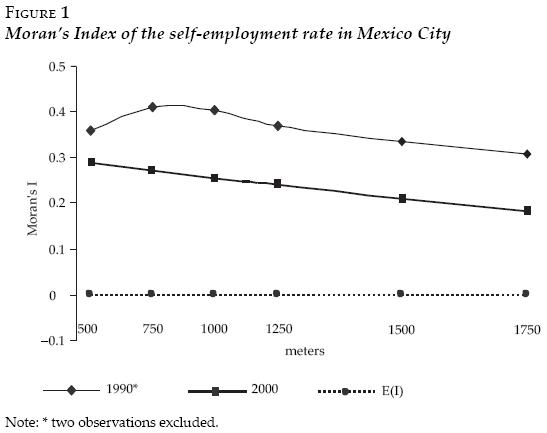
In order to have a better picture about local changes, the Local Indicators of Spatial Autocorrelation (lisa) were calculated at census tract level (see appendix for technical details). Figures 2, are the lisa maps of Mexico City for 1990 and 2000 respectively. The maps just highlight the clusters that are (pseudo) significant (p < 0.05) as indicated by random permutations. In the calculations, I use a band distance of 1 500 meters to construct the relevant physical distance network structure of the census tracts.
From figure 2, it can be appreciated that Mexico City depicts, broadly speaking, a spatial polarization in the rate of self–employment that evolved during the nineties. In 1990, there was a clear city division between west and east that defined the type of cluster formation: High–High census tracts were localized in the west side of the city (i.e., a census tract with an above average self–employment rate surrounded by census tract with above average self–employment), while Low–Low census tract were situated in the west side of the city in 1990 (i.e., a census tract below average surrounded by census tracts below average). In 2000, the city does not depict a strong west versus east division as in 1990. Exploration of the spatial data detects the following local changes: a) a strong High–High cluster in the south west in 1990 located in the Iztapalapa area, which is populated by blue–collar families, reduced substantially its cluster size in 2000; b) an important Low–Low cluster in the south west in 1990 that is localized in a middle class region practically vanishes from the picture in 2000. These changes by themselves can account for much of the reduction in the global spatial autocorrelation. That is, even though the rate of self–employment increased almost five points in the whole region, it seems that the spatial polarization is reduced at the same time. Nevertheless, strong spatial clusters remain in both years. A High–High cluster localized in downtown and a Low–Low cluster in the Northwest remain as important areas that exhibit significant spatial local autocorrelation. Interestingly, downtown High–High cluster spread toward Southwest in 2000 reaching middle class zones that were characterized by having Low–Low spots in 1990. This generated the emergence of a Low–High new region of spatial autocorrelation (i.e., a census tract with below average self–employment rate surrounded by census tract with above average self–employment). This situation opens the possibility to think that a possible process of diffusion might have taken place in that region.11
As indicated above, in the center of the city (downtown) there is an important cluster of spatial autocorrelation where rates of self–employment are quite above the average of the city (High–High census tracts). This area (historic downtown) is characterized by the presence of a strong informal economy (street peddlers) and has a rich tradition of small entrepreneurial activities in the service sector. Next, I will focus on this area.
Downtown area contains 299 census tracts and the average population per census tract in 2000 is 3428 habitants, while the average labor force per census tract is 1 504 persons. Table 1, displays the statistics of self–employment of the region and these are compared with those observed in the whole city. Note that the rate of self–employment is quite similar to that registered in the whole city either in 1990 or 2000; the Moran's Index in 1990 is also similar.12 But note that by 2000, the global indicator of spatial autocorrelation is larger in downtown than in the whole city; in other words, contrary to what happens in the whole city, the global spatial autocorrelation observed in downtown remains steady.
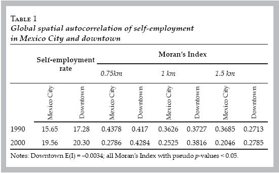
Figure 3 shows the lisa maps in 1990 and 2000 for the region studied using 1.4 km of distance. The main element in both figures is a strong division between a zone with High–High census tracts and a zone with Low–Low census tracts. Some of the highest growths in the self–employment rate are in the High–High cluster. This suggests, under a social contagion hypothesis, that the cluster is experiencing a positive feedback of increasing self–employment due to local interaction. Unfortunately, diffusion toward other areas is not perceived in the figure because the empirical analysis is restricted to downtown, but the High–High cluster extends Southwest (for details, see figure 2). It is true that the polarization looks stronger in 1990 than in 2000, but the landscape in 2000 remains divided, even when the self–employment rate grows globally in the region.
In the following section, I will introduce two models of social interaction that can explain the formation of spatial clusters in self–employment activities. Likewise, the models will be implemented empirically in the final sections of this essay through spatial econometrics and the framework of a census–tract model that combines Geographic Information Systems (GIS) and simulation.
A SIMPLE MODEL OF SOCIAL INTERACTIONS AT CENSUS TRACT LEVEL
Two different model specifications to study social interactions in self–employment decisions are studied: model A that considers simple imitation and model B that introduces a threshold rule. These two models are built up from the next relationship: self–employment in a census tract i (Si) is a function of the following variables: a) local information of the rate of self–employment of the neighbors (Sj) that are located inside a radius of distance (R) from census tract i; and b) a vector of own characteristics of census tract i (Xi):

If we follow the idea of a spatial reaction function (Brueckner, 2003), we have an interpretation of [1] as a solution of a maximization problem at census tract level. Suppose that each census tract has the objective function:

Therefore, each census tract i chooses the level of self–employment that maximizes equation [2] so that, Si =  U/Si = 0, which solution is equation [1]. Each census tract i chooses the best response given both its own characteristics (that define its preferences) and the choices of the other census tracts. It can be assumed that each census tract is a representative agent. I will work with a linear specification of relationship [1]. I consider that the rate of self–employment in the census tract is a continuous variable in the range [0, 1] and that each census tract i is a representative economic agent. Social interactions are implemented by using the average rate of self–employment that it is observed in the census tract neighbors that are within a radius of distance. Model A considers imitation through conforming to the average rate of self–employment in the neighborhood.
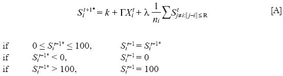
Where S is the rate of self–employment in census tract i, k is a constant, Γ is a vector of parameters associated to own characteristic variables of census tract i (education, sex, age, % of computers, etc.) and λ is the parameter associated to the rate of self–employment of the census tracts j's that are the neighbors of census tract i. Neighbors n are defined as those census tract j that are located inside a radius of distance R from i, the distance is taken from the centroid of the polygon representing the census tract. Note that when k = 0 and Γ = 0, the level of self–employment only depends on social interactions; when λ = 1, we have a case of strict imitation (replicating the average rate of self–employment of the neighborhood). Equation [A] is complemented by an error term per census tract. This implies that each time that a census tract reviews its rate of self–employment, a small £ exists such that a census tract i also considers other reasons than those that are explicit in the equation (the error accounts for unobservable).13 In contrast, in model B social interaction effects on self–employment are determined by threshold dynamics.14 Model B has two different laws of motion:

where N is the total number of census tracts.
Model B assumes that the underlying agents located in a census tract have a common perception that indicates that if the local rate of self–employment (neighborhood) is greater or equal than the global rate of self–employment (in the region), that would be enough to drastically increase the benefits for being engaged in self–employed activities. I assume that at each period, the global rate of self–employment is known (let us say that economic reports or local institutions make this information available). Each census tract i compares the global rate of self–employment with the rate of self–employment of its census tract neighbors and, if the rate of self–employment of the neighborhood is greater or equal than the global indicator, the census tract takes into account the rate of self–employment of its neighborhood; otherwise, the census tract updates its rate of self–employment without considering the rate of self–employment of the network. Equations [A] and [B] allow the introduction of two types of heterogeneity. First, both equations take into account census tract characteristics (such as sex, education, age, etc.). Secondly, specific spatial location of the census tract (the centroid of the polygon) and the radius of interaction among census tracts are the basic components of the physical network, which in the real world tends to be heterogeneous between census tracts. Geographic information systems provides data (Instituto Nacional de Estadística, Geografía e Informática, INEGI), to study empirically equations [A] and [B]. In particular, if equations [A] and [B] are considered simultaneously, a spatial econometric implementation exists using a Simultaneous Spatial Autoregressive (sar) parametric framework. In particular, a spatial lag model coincides with model A in a cross section setting (Anselin, 2001, 2002):

W is a weighting matrix (n x n) that formalizes the network structure and u is a vector of random errors, S is an n by 1 vector of self–employment rate observations, X is an n by k matrix of observations on the exogenous variables (i.e. census tract characteristics). Each element of W is row standardized such that Σjwij = 1, in that way premultiplying the vector of observations of neighbors (self–employment rate) by W corresponds to an averaging of the neighborhood values; in other words, equation [3] is a specification of imitation like in model A (but without subscript t).15 Model B can have also an econometric implementation (at cross section level) with a spatial lag model (equation [3]). This can be done with restricting neighbors not only to distance but also when the average level of self–employment of the neighborhood is equal or greater than the aggregate level of the region. The neighborhood structure can be reproduced in the W matrix of equation [3]: the only difference (with respect to the model of imitation) is that census tract j takes a value of zero in Wwhen the average rate of employment of the neighborhood is below the value of the aggregate rate of self–employment in the whole region considered.16
Due to econometric reasons that are considered in the next section, it is important to mention at this point, that the SAR framework has also another model in which the spatial dependence is incorporated in the error instead of the spatial lag variable as in equation [3]. If this were the case, the error in a linear specification to explain self employment rate could take the form of the following autoregressive model error:

where ε is a vector of i.i.d errors with variance σ2 and, W, S have the same characteristics than in the equation [3].
The differences on both models are apparent and, it is clear that the hypothesis of social interaction (imitation) only can be recovered in the spatial implementation of equation [3] where the spatial effect is incorporated in the spatial lag variable.
SPATIAL ECONOMETRIC IMPLEMENTATION OF THE MODELS (DOWNTOWN CASE)
In the last section, it was mentioned that the spatial lag model (equation [3]) can be considered as an econometric implementation of model A or B using cross section data. Consequently, equilibrium must be assumed when cross section data is used. In implementing the model, I have paid special attention to the exogenous variables: that is, the own characteristics of the census tract (vector X of observables in model A or B). Many variables associated to theories of self– employment mentioned before are considered. For example, I consider the percentage of the population per census tract that occupied their own house as proxy of assets.17 In the same way, the percentage of the population between 20–24 years old (young people) and the percentage of the population between 60–64 years old (old people) are used as proxies of the risk aversion hypothesis: less risk averse individuals are likely to become entrepreneurs and more risk averse are likely to become workers (Parker, 2004). To account for the quintessential determinants of the external labor market, I consider the average years of education for people over 15 years old per census tract and also the percentage of households that have computers as a proxy of human capital. Of course, these last variables bring supply and demand effects of the labor market into the setting. Along with the literature that evaluates self–employment as disguised unemployment, I use a rate of economic dependency that indicates the number of children (between 0 to 14 years old) and older people (above 65 years old) for each one hundred economically active persons (people between 15 to 64 years old). Finally, I consider the percentage of population who were living in the city 5 years ago as a variable that indirectly can control for some of the effects of sorting.18 It is important for the reader to remember that the data used for the self–employment variable in this research corresponds only to self–employed people working alone.19 All the mentioned variables are complemented by the social interaction variable that is the spatial lag variable in equation [3]: the rate of self–employment in each of the census tracts that are considered as neighbors (a distance criterion defines neighbors). The descriptive statistics of the mentioned variables in 2000 are displayed in table 2. As it is indicated above, all the variables except years of education and economic dependency represent percentages with respect to the population in the census tract.
Table 2 presents the mean and deviation of 299 census tract observations for downtown. In the third and fourth column of table 2, a join skewness/ kurtosis test for normality (an alternative to the Jarque–Bera test) is also presented (see D'Agostino et al., 1990). This test is known to follow a χ2 distribution with two degrees of freedom, and under the null hypothesis of normality, the expected value of the statistic is two. The results indicate clearly that all variables are far from being normally distributed (non–normality persist even when performing nonlinear transformations). The implications of this will be mentioned ahead.
If λ = 0 in the spatial lag model (see equation [3]), the econometric implementation of the models is reduced to an Ordinary Least Squares (OLS) estimation.
However, a previous section shows that the Moran's Index of the self–employment rate in the area studied presents significant spatial autocorrelation; ols estimation can be affected by this situation.20 Figure 4, shows the Moran's Index correlogram of the self–employment rate and the Moran's Index of the ols's residuals in different band distance.
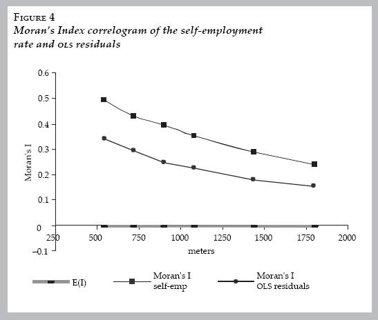
As expected, spatial autocorrelation is statistically significant also in the residuals of the ols regression (the regression without the lag variable). Note that the spatial autocorrelation is a monotonically decreasing function of physical distance. This situation alone could justify the use of a spatial lag model (equation [3]), however, the Moran's Index is also robust against misspecification problems (i.e. non–normality or hetereskodestacity). In fact, this is observed in the first column of table 4 where the diagnostic tests of the ols estimation of the model indicate non–normality in the errors and heteroskedasticity. Non–normality of the errors is not unexpected given that the covariates display strong non–normality (see table 2). It is important to mention that the violation of the normality hypothesis does not disqualify the model's specification when there are good theoretical reasons to think that there is a spatial model that is adequate (Arbia, 2006).21 Nevertheless, the problem of whether the spatial lag model is the best specification to account for the spatial autocorrelation remains, because, as it is known in the spatial econometric literature, a spatial error model (see equation [4]) can also account for the spatial autocorrelation as well. This is an important element to consider because the error can include omitted variables that are also spatially dependent.22
Therefore, several problems of identification can arise when a spatial (or social interaction) term is considered, and serious econometric work must be done to address these and other related problems. To respond to this issue, it is important to remark that in the last section, I showed that the spatial lag model (equation [3]) is an implementation of model A (or B) and, for that reason, it is not necessary to evaluate which econometric spatial model is more appropriate to account for spatial autocorrelation. Our motivations are theory driven not data driven. In spite of that and for information, I present the Lagrange Multiplier tests that allow for the distinction between spatial lag (LMlag) and spatial error (LMerror) model alternatives (see Anselin, 2001).23 Table 3, shows the main results for the tests.
Two different weight matrixes (W) of equation [3] are considered to calculate the tests: the first takes into account just local interaction (i.e., model A) and the second considers the threshold model (i.e., model B). As expected, all the standard Lagrange Multiplier tests accept the alternative.
Now, a simple rule sometimes used to distinguish between the alternatives when they are highly significant is to see which robust LM test has the higher statistic value (and which has the higher p–value); that is, if LMlag–rob > LMerror–rob then consider a spatial lag model otherwise go with the spatial error (Florax et al., 2003). In general and for the purposes of this exercise, the spatial lag seems to be well justified as an alternative.24 In general, the spatial lag model seems to be a better spatial option when the band distance is lower than one kilometer.
Table 4 summarizes the main results of the regressions considering only model A. The first column of the table displays ols results of the specification (not considering the social interaction term) and in the second column is reported estimation with robust errors; likewise in the third and fourth columns, a reduced ols version of the model is estimated. The next columns of table 4 report the estimation of the spatial lag model by maximum likelihood considering different band distances. The spatial lag estimations also report robust error estimation but it is only showed for the reduced model when the band distance is 540 meters. The spatial lag estimations are based on the algorithms outlined in Smirnov and Anselin (2001) implemented in Geoda 0.9.5–i(beta) and the robust versions were calculated in Data Analysis and Statistical Software (STATA) using the procedures of Maurizio Pisati (2001).25
Likewise, table 5 summarizes the main results of the regressions considering model B without reporting the robust and the reduced version of the models.26
First of all, table 4 and 5 indicate that the spatial lag model in both models fits better the data than ols as it can be corroborated through the log likelihoods; but most importantly, the spatial interaction term is highly significant and positive in either spatial lag model (A or B) and, its inclusion is affecting the estimation of the covariate coefficients. Nevertheless, the social interaction coefficient in model A (local interaction) is more than twice than the value of the coefficient in model B (threshold).
The spatial lag models still have problems of heteroskedasticity as indicated by the Breusch–Pagan test, but this is not unexpected given that the data presents strong non–normality.27 Nevertheless, note that a robust estimation (see column called robust in table 4) do not change substantially the results. Moreover, the presence of heteroskedasticity can be in part due to the fact that some of the sociodemographic covariates used in the analysis presumably are correlated. To consider this, see in table 4 that heteroskedasticity is not present either in the ols reduced version or in the spatial lag model reduced version as it is indicated by the Koenker–Basset (KB) test and the Breusch–Pagan test respectively. However, non–normality continues being present in the model because the kb test does not rely on the assumption of normality. It is important to mention that significant changes in the social interaction term are not detected even when the robust and the reduced models are considered; for that reason, we consider that the results will no be drastically modified if more sophisticated and complex spatial methods that deal with non–normality were implemented. Similar conclusions have been reached in other researches that deal with similar characteristics in the data used in this essay (see Mobley et al., 2006).
The important result of this spatial econometric exercise has been to show that the spatial interaction term is significant, but also it is important to mention some results of the covariate coefficients. Contrary to what the literature of entrepreneurship would expect (Evans and Jovanovic, 1989), liquidity constraints (see own house variable) has a null or negative impact on the rate of self–employment (both models produce similar results). Education is strongly significant and negatively correlated to self–employment and that economically dependent persons (children and elders) are significant with positive coefficient. The negative impact of education is consistent with other empirical studies that use micro–data to analyze entry–exit decisions on self–employment in Mexico (Woodruff, 1999). 28
Another interesting result is that the rate of old people (60–65 years old) is consistently positive and statistically significant; this situation reinforces the hypothesis that conditions of poverty and weak or absent social security for the elderly increases the rate of self–employment. Also note that the proportion of the population living in the city in 1995 tends to be statistically significant in most of the band–distances. This variable controls indirectly for sorting effects. In general, similar results are produced by models A and B in the statistical significance and sign of the parameters. But the social interaction term differs strongly in magnitude between models: local interaction is in average four times larger than the parameter obtained in the threshold model. The rest of the covariates do not exhibit large discrepancies in magnitude between models, but the parameter of education is stronger in the threshold model. Maybe the important suggestion in the regression data would be that global information in Model B plays a role of stabilizer in the sense that it diminishes the effect of local interactions reflected in the size of the coefficients. If the threshold model is a proxy of the way in which institutions (or policy effects by the authority) are being incorporated at individual level (census tract), then the smaller magnitude in the social interaction term in model B might be consistent with the idea that institutions reduce uncertainty in the economic environment (North, 1990).
It is important to remark that I am not claiming identification of the social interaction term with the spatial econometric implementation. Problems of identification in these kinds of models are hard in cross–sectional settings (Manski. 1997). Nevertheless, the spatial lag model is a suitable econometric implementation that provides us with relevant information that enriches the simulation procedures of our models. Empirical issues (and calibration of the models) will be further addressed in the next section in a simulation framework.
SIMULATION, CLUSTER DYNAMICS AND EMPIRICAL ADEQUACY OF THE MODEL
Dynamics properties of the models are not possible to study in a spatial lag econometric framework. But the spatial lag implementation provides information to restrict parameter space in the census tract simulations and, with that, the possibility to analyze the dynamic properties of the models. Specifically, the simulations in the next section are designed to see how well the models match the global Moran's Index empirically observed in the self–employment rate in downtown Mexico City in 2000.
Conditions of the model
The average rate of self–employment per census tract observed in downtown is 19.72 (the aggregate self–employment rate in the area is 20.3).29 In the simulations, I target an equilibrium outcome that is close to the average rate of self–employment observed in 2000. In order to replicate this equilibrium outcome, I use the information provided by the spatial lag model in cross section, which presumes to be at equilibrium, to restrict parameter space in models A and B.30
It is observed from tables 4 and 5 that the best fit (see log likelihood) in both models happens in general in the distances: 540, 720, and 900 meters. In the simulations, I use the mean value of the parameters of the spatial lag model that are generated in these distances. I am assuming that the values of the parameters are not affected by distance. Because the basic idea of the simulations is to evaluate the dynamics of global clustering that each model produces, I will use the Moran's Index calculated at equilibrium to monitor the global spatial autocorrelation of the self–employment rate in the region at each period of time. An error is also considered in the simulations. To implement that, each census tract incorporates an error that comes from a normal distribution with standard error equal to the average of the standard errors of the spatial lag model and with mean zero. Also, all census tracts adjust asynchronously their rate of self–employment once each period of time.31 The initial conditions used are the empirical observations of the rate of self–employment in 2000, but this is somewhat irrelevant because random initial conditions do not affect the general results. Finally, information of the own characteristics of the census tracts comes from census data in 2000.
Results
The simulations with noise do not produce a fixed equilibrium (either in the Moran's Index or the rate of self–employment) but one that oscillates very close around a gravitational point. I average the Moran's Indexes generated in 200 periods of time (more periods of times do not statistically affect the results) in order to have an estimate to compare with. First, I contrast in Figure 5, the models with and without an error term.
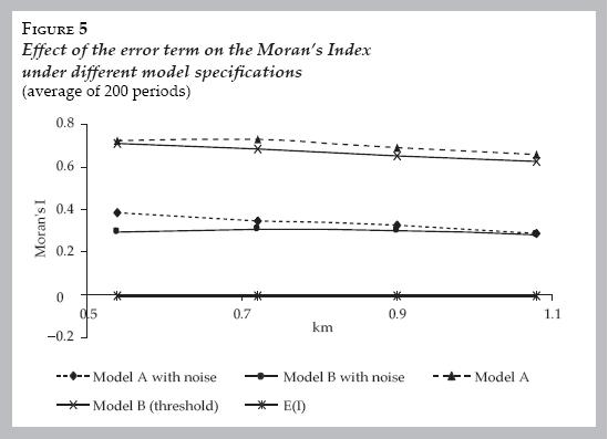
What random components do is essentially diminish the level of global spatial autocorrelation in the region simulated. The Moran's Index in both models drops more than twice if compared when noise is not present but it continues to show high and statistically significant levels of positive spatial autocorrelation.32 Nevertheless, in our models the Moran's Indexes continue to show strong spatial autocorrelation because pure local interaction (model A) or global–local interaction (model B) in conjunction with the other variables (i.e., census tracts' own characteristics) counterbalances the effect of noise maintaining the spatial clustering. The important result is that spatial autocorrelation of the self–employment rate continues being statistically significant even with random shocks. Now it is important to ask whether the models are reproducing the global spatial autocorrelation empirically observed in the self–employment rate. If we assume that the self–employment rate observed in 2000 is at equilibrium, then we can compare its Moran's Index with the one produced by the models. Figure 6 displays these comparative results between models and empirical data. The figure also contains a series of the models without the social interaction term (no local interaction or no global–local interaction effects) and that were produced with ols estimation (i.e., no social interaction term).
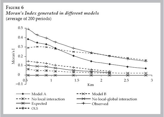
First, note that models of pure local interaction and threshold are much closer to the empirical data than the rest of the specifications. Then, a simple comparative static exercise indicates that the social interaction term is fundamental to reproduce the spatial autocorrelation observed. It is true that in short band distances (less than 1.5 km), the series without the social interaction term produce statistically significant spatial autocorrelation (own characteristics and error contribute to that), but they are quite low to be close to what is empirically observed. This gives an insight regarding the role of pure local interactions: it happens that local conformity under the presence of own characteristics variables triggers spatial autocorrelation.
Spatial autocorrelation of self–employment decreases in all models as the distance increases. But while it is clear that the models without the social interaction term reach spatial randomness with relatively short band distances, this situation does not occur with models A or B.
The dynamics of model A and B display interesting dynamics in figure 6, model A (local conformity) produces higher spatial autocorrelation than model B when the distance is smaller than 1 km; consequently, the series are closer to the empirical spatial autocorrelation. This is consistent with the results of the econometric implementation (see last section) where model A has a better fit than model B in these band distances. But, interestingly, the behavior of both models is reversed if the band of distance is greater than 1 km: model B (threshold) not only produces higher spatial autocorrelation but its simulated outcomes are also close to the empirical ones.
From the point of view of reproducing local clusters, the latter results are consistent with local Moran's Index. In figure 7, I show typical lisa maps realizations of simulations in models A and B and ols specification (initial conditions are random in all models). The simulated maps are contrasted with the empirical one. I highlight lisa statistics with 1% pseudo–significance level and the band distance used is 1 800 meters.

From figure 7, it is clear that models A and B reproduce better the empirical cluster than the ols specification, which does not include the social interaction term. But model B (threshold) seems to reproduce better the empirical cluster. The local results are consistent with the global spatial autocorrelation generated by the models in these particular realizations: Model B generates the highest Moran's Index (0.183), which is closer to the empirical one (0.2404).
The main lesson of the simulations is that a model that considers global–local information (model B) fits real data better than a simple model of local information if a relatively large distance network structure is influencing the rate of self–employment (more than 1.5 km). This suggests, given the assumptions of model B, that self–employment rates at census tract level not only are influenced by local information (provided by the neighborhood), but also by global entities that process global information. Governmental propaganda, publicity and activism of local leaders can be means of transmission of global information.33
If both formal and informal institutions are processing and returning global information to the system, they can reduce the uncertainty about the global environment (i.e., less global spatial autocorrelation). At the same time, they are perpetuating polarization in the clusters (i.e., an increase of the local spatial clusters). This conclusion is consistent with the notion of local conformity and global diversity postulated by the literature of social interactions and institutions (Young, 1998).
CONCLUDING REMARKS
This research contributes to understanding self–employment in developing countries because it advances a hypothesis so far not considered in the literature: entry–exit decisions in self–employment activities are also influenced by non–market interactions. In particular, this paper proposed through implementing a census tract based model with data of downtown Mexico City from 2000 that increasing returns from conformity are present in individuals when they are facing entry–exit decisions in the self–employment sector. Likewise, in this essay it is suggested that the effect of social influence must not be only restricted to local informational dynamics (neighborhoods) because channels of global information can also shape the effects of social influence. This situation remits us to the possibility that a threshold behavior might be present in the decisions of entry in self–employment activities; a situation that is reminiscent of social scientists understanding of collective action phenomena (such as joining a revolt, voting for a party, etc.).
An additional point is that the presence of social contagion in self–employment activities must not be restricted only to environments where informality and poverty are common (like Mexico City); the thesis certainly must apply in more advanced countries too. Further research in this area is necessary. Due to lack of information, this study relies on census tract data for the year 2000. However, the methodology of this paper might be adjusted to incorporate household level data and better information set regarding entry–exit decisions in self–employment. Further research must address this possibility. Finally, the fact that social interactions can be present in self–employment activities can have strong policy implications to either boost entrepreneurship or to combat poverty traps; moreover, the fact that our results indicate that social interactions in self–employment entry–exit decisions operate through channels of local and global information, raises the issue of the viability of the authorities intervention to regulate the phenomena. However, in order to figure out the way in which policy could be effective, it is necessary to have more precise micro information of the local dynamics.
REFERENCES
Anselin, L., Local indicators of spatial association: LISA, Geographical Analysis, vol. 27, no. 2, 1995, pp. 93–115. [ Links ]
Anselin, L, Spatial econometrics, inB. Baltagi (ed.), A Companion to Theoretical Econometrics, Oxford, Basil Blackwell, 2001, pp. 310–330. [ Links ]
Anselin, L., Under the hood. Issues in the specification and interpretation of spatial regression models, Agricultural Economics, vol. 27, no. 3, 2002, pp. 247–267. [ Links ]
Arbia, G., Spatial Econometrics, Berlin, Springer, 2006. [ Links ]
Arrow, K.J. and R. Borzekowski, Limited network connections and the distribution of wages, The Federal Reserve Board, Finance and Economics Discussion Series, Working Paper no. 2004–41, 2004. [ Links ]
Brueckner, J.K., Strategic interaction among governments: an overview of empirical studies, International Regional Science Review, vol. 26, 2003, pp. 175–188. [ Links ]
Calderón–Madrid, A., Job stability and labor mobility in urban Mexico: a study based on duration models and transition analysis, Inter–American Development Bank, Research Network, Working Paper no. R–419, 2000. [ Links ]
Case, A.C., Spatial patterns in household demand, Econometrica, vol. 59, 1991, pp. 953–965. [ Links ]
Calvó–Armengol, A. and M. Jackson, The effects of social networks on employment and inequality, American Economic Review, vol. 94, 2004, pp. 426–454. [ Links ]
D'Agostino, R.B., A. Balanger and R.B. D'Agostino Jr., A suggestion for using powerful and informative tests of normality, American Statistician, vol. 44, 1990, pp. 316–321. [ Links ]
De Soto, H., The Other Path, New York, Basic Books, 1989. [ Links ]
Eatwell, J., Effective demand and disguised unemployment, in J. Michie and J. Grieve Smith (eds.), Employment and Economic Performance:jobs, inflation and growth, Oxford, Oxford University Press, 1997. [ Links ]
Evans, D.S. and B. Jovanovic, An estimated model of entrepreneurial choice under liquidity constraints, Journal of Political Economy, vol. 97, 1989, pp. 808–827. [ Links ]
Florax, J.G.M., H. Folmer and S.J. Rey, Specification searches in spatial econometrics: the relevance of Hendry's methodology, Regional Science and Urban Economics, vol. 33, 2003, pp. 557–579. [ Links ]
Galli, R. and D. Kucera, Informal employment in Latin America: movements over business cycles and the effects of worker rights, International Institute for Labour Studies, Discussion Paper no. 145, 2003. [ Links ]
Giannetti, M. and A. Simonov, On the determinants of entrepreneurial activity: individual characteristics, economic environment and social norms, Swedish Economic Policy Review, vol. 11, no. 2, 2004, pp. 269–313. [ Links ]
Glaeser, E.L., B.I. Sacerdote and J.A. Scheinkman, The social multiplier, Journal of the European Economic Association, vol. 1, no. 2–3, 2003, pp. 345–353. [ Links ]
Granovetter, M., Threshold models of diffusion and collective behavior, American Journal of Soáology, vol. 83, 1978, pp. 1420–1443. [ Links ]
Granovetter, M., The economic sociology of firms and entrepreneurs, in A. Portes (ed.), The Economic Sociology of Immigration, New York, Russell Sage Foundation, 1995. [ Links ]
Harris, J.R. and M.P. Todaro, Migration, unemployment and development: a two sector analysis, American Economic Review, vol. 60, no. 1, 1970, pp. 126–142. [ Links ]
Hurst, E. and A. Lusardi, Liquidity constraints, household wealth and entrepreneurship, Journal of Political Economy, vol. 112, 2004, pp. 319–347. [ Links ]
Ianni, A. and V. Corradi, The dynamics of public opinion under majority rules, Review of Economic Design, vol. 7, 2002, pp. 257–277. [ Links ]
Instituto Nacional de Estadística, Geografía e Informática (INEGI), Sistema para la Consulta de Información Censal (SCINCE) 1990 and 2000 (compact disc). [ Links ]
Light, I. and C. Rosenstein, Expanding the interaction theory of entrepreneurship, in A. Portes (ed.), The Economic Sociology of Immigration, New York, Russell Sage Foundation, 1995. [ Links ]
Lucas, R.E. Jr., On the size distribution of business firms, BellJournalof Economics, vol. 9, 1978, pp. 508–523. [ Links ]
Maloney, WF., 'Informality revisited, World Devebpment, vol. 32, 2004, pp. 1159–1178. [ Links ]
Manski, C.F., Identification of anonymous endogenous interactions, in WB. Arthur, S.N. Durlauf and D.A. Lane (eds.), The Economy as an Evolving Complex System II, United States, Addison–Wesley, 1997, pp. 369–384. [ Links ]
Mobley, L.R. et al., Spatial analysis of elderly access to primary care services, International Journal of Health Geographics, vol. 5, no. 19, 2006. [ Links ]
North, D.C., Institutions, Institutional Change and Economic Performance. Cambridge, Cambridge University Press, 1990. [ Links ]
Parker, S.C., The Economics of Self–employment & Entrepreneurship, Cambridge, Cambridge University Press, 2004. [ Links ]
Piore, M. (ed.), Unemployment and Inflation, White Plains, M.E. Sharpe, 1979. [ Links ]
Pisati, M., Tools for spatial data analysis, Stata Technical Bulletin, no. 60, 2001, pp. 21–37 [ Links ]
Portes, A. and P. Landolt, Social capital: promise and pitfalls of its role in development, Journal of latin American Studies, vol. 32, 2000, pp. 529–547. [ Links ]
Salas, C., Trayectorias laborales entre el empleo, el desempleo y las microunidades en México, Papeles de Población, no. 38, 2003, pp. 121–157. [ Links ]
Schelling, T., Micromotives and Macrobehavior, United States, WW Norton & Company, 1978. [ Links ]
Semmler, W, On the mechanisms of inequality, Center for Empirical Macroeconomics, Department of Economics, University of Bielefeld, Working Paper no. 134 2003. [ Links ]
Smirnov, O. and L. Anselin, Fast maximum likelihood estimation of very large spatial autoregressive models: a characteristic polynomial approach, Computational Statistics and Data Analysis, vol. 35, 2001, pp. 301–319. [ Links ]
Tobler, W, A computer movie simulating urban growth in the Detroit region, Economic Geography, vol. 46, 1970, pp. 234–240. [ Links ]
Topa, G., Social interactions, local spillovers and unemployment, Review of Economic Studies, vol. 68, 2001, pp. 261–295. [ Links ]
Woodruff, Ch., Can any small firm grow up? Entrepreneurship and family background in Mexico, Graduate School of International Relations and Pacific Studies, University of California, Working Paper, 1999. [ Links ]
Young, H.P., Individual Strategy and Sodal Structure, Princeton, Princeton University Press, 1998. [ Links ]
* The author thanks two anonymous reviewers for constructive comments and suggestions.
1 The self–employment rate in Mexico City is 20% in 2000.
2 This line of thought is not so far from that delineated in De Soto (1989).
3 The official unemployment urban rate in Mexico is between 2 and 3 per cent.
4 Another common reference with dualistic or segmented labor markets is the so called Harris–Todaro model (1970) for developing countries that is built up through considering wage differentials between sectors.
5 The main point is that movements of informal employment are countercyclical: it increases in downturns absorbing workers form formal sector and decreases in upturns.
6 For example, President Fox of Mexico (2000–2006) promoted self–employment activities (changarnos) among the poor and lower middle–class.
7 See appendix for details.
8 In this research only the part of the city that corresponds to the capital of the country is considered, that is, the Distrito Federal (DF).
9 The self–employment rate is defined as the percentage of self–employed persons (working alone) over the population economically active (labor force). The population economically active is defined as the population over 12 years old that worked or sought job during the week of the interview
10 All indexes are pseudo–significant: p < 0.01, inference based on 999 permutations.
11 It is part of the popular wisdom that the crisis of 1995 in Mexico (an in general the poor economic performance in Mexico during the 1990s) strongly impacted the middle–class. At least the aggregate data of this research suggests that middle–class zones started to be more engaged in self–employed activities. Moreover, the results run along the buffer hypothesis that indicates that self–employment is countercyclical.
12 In 1.5 km the Moran's Index diminishes in downtown because the area analyzed is much smaller.
13 In the econometric literature of social interaction, equations that are similar to [A] can be found in Topa (2001) (implemented also at census tract level) and in Glaeser, Sacerdote and Scheinkman (2003), who treat the relationship at the individual level in a cross section setting and where the social interaction refers to an aggregate of a reference group instead of an aggregate given by physical distance like in this case.
14 Thresholds models, where collective behavior becomes influential in individual decisions only if a certain value (or level of tolerance) is surpassed, have been proposed to analyze a wide variety of social phenomena such as social revolts, residential segregation, informational cascades, etc. (Schelling, 1978; Granovetter, 1978). This type of modeling in the context of self–employment could take into account the costs associated to the perception that many (or few people) are enrolled in self–employed activities. Likewise, another important justification of proposing a threshold model in self–employment (that is not restrictive to developing countries) is related to the thresholds models of skill formation that have been proposed to explain locally increasing returns in growth theory (Semmler, 2003).
15 Note that in equation [3], dSi/d Sj = XW, which corresponds to the second partial derivative of equation [1].
16 There is a cost in doing this and it is that the W matrix generates necessarily 'islands' (zero rows); this can complicate inferential procedures (Anselin, 2002).
17 The central issue in the standard theory of entrepreneurship is that individuals with greater assets are more likely to become self–employers (Evans and Jonavovic, 1989).
18 Family income was excluded because it is not a census tract characteristic that can be considered exogenous like the other variables in the specification.
19 With this regard, Woodruff (1999), in a working paper, has suggested that the determinants of self–employment in Mexico differ between a self–employer working alone and those with workers (or employers). The latter are the only ones that tend to behave along the lines of the theories of self–employment proposed in developed countries.
20 OLS produce biased and inconsistent estimations.
21 Likewise, presence of no/ normality and heteroskedasticity are frequent in this kind of settings because both are related problems (Arbia, 2006)
22 When using a spatial lag model [3], many precautions must be taken because spatial autocorrelation can be due to either the neighbors' influence (i.e., social interaction) or the errors (omitted variables) (see equation [4]). Moreover, the spatial autocorrelation can be due to both effects (see Case, 1991, for an implementation that nests both effects). Several methodological strategies can be cited to deal with this potential problem of specification (Case, 1991; Florax, Folmer and Rey, 2003; Anselin, 2002).
23 These statistics have both an asymptotic χ2 distribution with one degree of freedom. In strict sense, these tests would not be robust because they depend on errors that are normal. Nevertheless, we report the results because they provide useful information for this research; moreover, it is not uncommon to find in empirical essays the use of these tests even when the data shows non–normality (Mobley et al., 2006).
24 The tests are only informative because it is difficult to distinguish alternatives if we rely on them.
25 Because two different programs are used in the estimation of the spatial lag model, the estimation of coefficients are not identical between them. However these discrepancies are not significant for the purposes of this exercise.
26 I do not report these two last estimations because once they are considered in the model, the results behave similarly as in model A. In any case, the results can be obtained upon request.
27 Heteroskedasticity is not uncommon when dealing with regional data because of the irregular nature of the areas (or regions) analyzed (Arbia, 2006). Heteroskedasticity can also indicate that different spatial regimes must be considered; however, we dismiss this possibility because the area analyzed is relatively small (a portion of Mexico City).
28 Calderón–Madrid (2000) using panel data for Mexico between 1995–98 (and calculating hazard rates from leaving one sector to another) found that people with formal and higher education spend less time in self–employed activities.
29 These rates do not differ from the rates observed in the whole city —see table 1.
30 I showed previously that the spatial lag model identifies appropriately model A and B.
31 This is equivalent to a uniform activation of the census tracts, which means that a census tract i acts immediately before census tract j over the course of a period of time.
32 The loss of spatial autocorrelation when noise is present is in accordance with what the theoretical literature of social interactions has suggested when random behavior is introduced in systems that resemble the one analyzed in this research: noise is breaking out the clusters formed in systems based on local information (see Young, 1998; Ianni and Corradi, 2002).
33 For example, the political power of the leaders of the street peddlers in downtown Mexico City is widely recognized. Likewise, the federal governmental propaganda to promote self–employed activities (changarros) are also well recognized.

