Artículos

 

Inflation, Output and Economic Policy in Mexico

 

Inflación, crecimiento y política económica en México

 

Víctor M. Cuevas Ahumada*

 

* Universidad Autónoma Metropolitana-Azcapotzalco, <victorcuevasahumada@yahoo.com.mx>.

 

Received May 2007
Accepted January 2008.

 

Abstract

This paper investigates the leading sources of inflationary pressure and output variations in the Mexican economy. To this end, we make use of a multivariate error-correction model, which is consistent with a small open economy with a floating exchange rate system. As our object is to let the data expose the key determinants of prices and output, we resort to a broad aggregate demand-aggregate supply model consisting of three markets: goods, money, and labor. Taken as a whole, the empirical evidence suggests that monetary expansions are basically accommodated through a higher price level, rather than a higher economic activity. In the short run, real exchange rate depreciations produce a moderate effect on inflation and an insignificant effect on output. In the long run, however, an undervalued currency results in production losses. In addition, we find that i) both inertial inflation and inflationary expectations are among the driving forces of price instability, and ii) shocks to nominal wages are recessionary at impact and this negative effect is persistent over time. Lastly, nominal wages are a positive function of capacity utilization and the expected rate of inflation, thereby suggesting a forward-looking wage adjustment process. As we shall see, these findings have some relevant implications not only for the monetary and the exchange rate policies, but also for the so-called central bank's credibility.

Key words: inflation, output, monetary policy, error-correction model.

Clasificación JEL: C32, E12, E52

 

Resumen

El presente trabajo analiza las principales fuentes de inflación y de variación en la producción en la economía mexicana. Para ello, se recurre a un modelo multivariado de corrección de errores, que es consistente con una economía pequeña, abierta y con un régimen cambiario flexible. Con el fin de permitir que los datos hablen por sí mismos, aquí se hace uso de un modelo amplio de oferta y demanda agregadas consistente de tres mercados: de bienes, de dinero y laboral. En términos generales, el cuerpo de la evidencia empírica sugiere que las expansiones monetarias, más que traducirse en una mayor actividad económica, se traducen en una mayor inflación. En el corto plazo, las depreciaciones reales de la moneda generan un efecto moderado en los precios y un efecto demasiado tenue en la producción. En el largo plazo, sin embargo, un tipo de cambio subvaluado desincentiva la actividad productiva. Por otra parte, existen claros indicios de que: i) tanto la inflación inercial como las expectativas inflacionarias se encuentran entre los principales motores del crecimiento de los precios, y ii) los choques salariales surten efectos recesivos inmediatos y de larga duración. Finalmente, los salarios nominales son una función creciente no sólo de la capacidad instalada utilizada sino de la tasa de inflación esperada, lo cual es indicativo de que los salarios se ajustan, hasta cierto punto, con una visión ex ante. Como habrá de verse, estos hallazgos revisten importantes implicaciones tanto para las políticas monetaria y cambiaria, como para la credibilidad de la Banca Central.

Palabras clave: inflación, producción, política monetaria, modelo de corrección de errores.

 

Introduction

This paper investigates the key sources of inflation and output fluctuations in the Mexican economy. To accomplish this task, we rely on a multivariate Vector Error-correction (VEC) model, which is consistent with a small open economy with a flexible exchange rate. As the purpose here is to let the data reveal the basic determinants of prices and output, we make use of a broad aggregate demand-aggregate supply model composed of three markets: goods, money, and labor.¹

Since January 2001, the Mexican monetary policy has been conducted within a full-fledged inflation targeting framework. The basic features of this regime are: i) the central bank is independent of the federal government is given the mandate of achieving price stability, ii) the monetary authority systematically commits itself to comply with a previously announced inflation target, but enjoys leeway in the formulation and implementation of monetary policy, iii) monetary policy makers convey ample information concerning not only the short- and long-term inflation targets, but also the policy tools that will be employed to accomplish them, and iv) the overall central bank's governance structure, the setting of quantitative inflation targets and ranges,² and the communication strategy regarding the goals and means of monetary policy, induce high standards of transparency and accountability.

In this context, the effectiveness of monetary policy requires the specification of attainable targets and, therefore, the continuous generation of empirical studies with regard to the underlying sources of inflation, the responsiveness of prices and output to different types of policy actions, and the lags between policy changes and inflationary outcomes. Consequently, this research focuses on the basic determinants of inflation and output variations, thereby contributing to the current debate on what causes price instability and how to improve inflation performance.

The overall evidence suggests that money supply is an important source of short- and long-run inflation. In particular, we find that unexpected monetary expansions are mostly accommodated through an increasing price level, rather than an increasing production. In the short run, a real currency depreciation results in a moderate effect on inflation and a negligible effect on economic activity.³ In the long run, however, the real exchange rate is negatively related with output. Shocks to wages produce an immediate and long-lived recessionary effect, but they do not have a clear repercussion on prices. It is also shown that the behavior of prices entails a robust predetermined component (or inflationary inertia) and that higher inflationary expectations may affect the price level, making the realization of the inflation target more difficult for the Mexican central bank.

By the same token, there is solid empirical support for the notion that nominal wages respond in a positive way to increases in both capacity utilization and expected inflation. As we shall see, this particular finding has an important policy implication for the Bank of Mexico.

The paper is organized as follows. Section I provides a brief review of the empirical literature on the subject. Section II presents the theoretical model. Section III analyses the data, econometric methodology, and empirical results. Finally, as part of the conclusions, we summarize the findings and explore the policy implications.

 

Review of the literature

There are a number of empirical papers investigating the determinants of inflation in Mexico. Nonetheless, only a few of them examine the sources of output fluctuations as well. There is also some empirical work specifically related to the so-called pass-through effect from exchange rate to prices. This particular line of research focuses on the link between exchange rate depreciation and inflation, leaving other variables out of the analysis.

One of the pioneer empirical analyses of the Mexican inflationary phenomenon is Yacaman (1982). This author investigates how different macroeconomic variables (such as excess money supply, wages, expected inflation and foreign inflation) affect the domestic inflation rate. Based on regression analysis, he concludes that the only permanent or long-run source of inflationary pressure is an excess money supply. In the short-run, however, he finds that supply-side shocks, such as wage increases or a higher-than-expected international inflation, can create price instability. Finally, the evidence submitted indicates that, as inflation accelerated during the 1970s, the contribution of imported inflation to the home-country's inflation almost doubled while the contribution of wages was practically cut in half.⁴

Arias and Guerrero (1988), on the other hand, develop a six-variable (domestic price level; foreign price level; effective exchange rate; money supply as a share of Gross Domestic Product, GDP; public sector prices, and wages) Vector Autoregression (VAR) model to gather additional eviden about the underlying causes of inflation in Mexico. They choose a sample period characterized by an increasing inflation rate (1970-1987) and prove that both the exchange rate and foreign prices are significant sources of price instability. This result reinforces Yacaman's conclusion regarding the prominent role played by imported inflation during the 1970s. Unlike Yacaman (1982), however, these authors state that wages do not really exert a significant influence on inflation. Monetary disturbances display permanent but relatively small effects on inflation, whereas public sector prices have a strong but short-lived inflationary effect. Lastly, Arias and Guerrero (1988) point out the presence of a growing inflationary inertia during those years.

Dornbusch et al. (1990) emphasize that exchange rate shocks are a leading inflationary factor in developing countries. They utilize a three-variable (inflation, real exchange rate, and real budget deficit) VAR model to conduct a multi-country empirical analysis of inflation, which includes Argentina, Brazil, Peru, Bolivia and Mexico. According to these authors, the exchange rate is a strong determinant of inflation in Argentina, Brazil, Mexico and Peru, but not as much in Bolivia. The budget deficit seems to be influencing prices only in Mexico, Bolivia and Peru. In contrast, Argentina and Brazil yield robust evidence of fiscal endogeneity, given the passive reaction of their budget deficits to shocks in the other two variables of the system. Moreover, inflationary dynamics in these two countries is driven by a combination of exchange rate shocks and inertial inflation. In the Mexican case, nevertheless, inflationary inertia appears to be relatively low.

Wang and Rogers (1994) utilize a five-variable (budget deficit, output, prices, real exchange rate and real money balances) VAR model to examine the responsiveness of prices and output to different types of shocks in the Mexican economy. They conclude that fiscal and monetary shocks have more influence on prices than do exchange rate shocks. Furthermore, output fluctuations are mainly determined by real and fiscal shocks, whereas monetary expansions and exchange rate depreciation do not exhibit significant real effects.⁵

Relying on a micro-based macroeconomic model and regression analysis techniques, Perez-Lopez (1996) shows that the behavior of the Mexican inflation rate can be adequately captured by a markup model whose explanatory variables are: the rate of change in wages, the rate of change in external prices expressed in domestic currency, and lags of both the dependent variable {i.e., the inflation rate) and the two independent variables. Thus, the evidence rendered here indicates that the domestic rate of inflation is sensitive to wage increases, nominal exchange rate depreciation, and inflation abroad. A slightly modified version of this markup model of inflation, on the other hand, has been used by Garces (1999) and Bailliu et al. (2003), mainly to formulate inflationary forecasts. It is worth mentioning that Bailliu et al. (2003) show that, in terms of forecasting power, their markup model outperforms the money gap and the open-economy Phillips curve models.

Agenor and Hoffmaister (1997) conduct a multi-country empirical investigation which comprises Chile, Korea, Mexico, and Turkey. The variables selected for each country are: inflation, money growth, nominal exchange rate depreciation, nominal wage growth, and the output gap. Using the generalized VAR approach, which is useful to make the empirical evidence independent of the VAR ordering, they demonstrate that wage shocks feed inflation in all countries, but the inflationary outcome is particularly persistent in Korea and Mexico.⁶ Exchange rate depreciation is inflationary in Mexico, Chile and Turkey, but not in Korea. A monetary impulse leads to higher output and inflation in all economies. In the Mexican case, nonetheless, an increase in the nominal money stock has a long-lived effect on prices and a merely transitory effect on economic activity.

Baqueiro, Díaz de León and Torres (2003) investigate the pass-through effect from exchange rate to prices in Mexico and other fifteen small open economies with flexible exchange rates. The empirical results are very robust in terms of revealing a direct relationship between the inflation rate and the magnitude of the pass-through effect. Put differently, the evidence strongly suggests that, as these economies move from a high-inflation to a low-inflation scenario, the influence of exchange rate fluctuations on the price level decreases. The above is consistent with previous research in the area, which highlights the significant contribution of foreign prices and the exchange rate to the domestic inflation rate during the high-inflation episodes (Yacamán, 1982; Arias and Guerrero, 1988; Dornbusch et al., 1990; Pérez-López, 1996; Agénor and Hoffmaister, 1997).⁷

Using different econometric techniques, Galindo and Catalán (2004) provide evidence indicating a strong positive relationship between the four monetary aggregates and the rate of inflation. Furthermore, they show that monetary expansions could eventually lead to higher output, but emphasize that the relationship between money and economic activity is more complex and less robust than the relationship between money and prices.

Finally, on the basis of a six-variable (budget deficit, monetary base, real exchange rate, real interest rate, price level and output) VAR model, Cuevas (2005) shows that real exchange rate depreciation continues to be an important source of cost-push inflation in the Mexican economy, even though the time series used correspond mainly to the recent low-inflation period. An unexpected monetary expansion, on the other hand, results in a lower real interest rate and a higher output in the short run, which is consistent with the so-called liquidity effect. Finally, a rise in the government budget deficit has an indeterminate effect on output and a positive but negligible effect on prices.

In conclusion, the empirical literature identifies several variables as potential sources of inflation in Mexico and other developing countries: budget deficit, money supply, exchange rate, foreign prices, wages, public sector prices, inflationary expectations, and the output gap. The whole evidence put forward suggests that some of these variables influence economic activity as well. As we shall see, the model developed in this paper includes most of the aforementioned variables.

 

Theoretical framework

This section lays the foundation for a model consisting of nine observable variables: government spending (g_t), money supply (m_t), domestic nominal interest rate (i_t), real exchange rate (q_t), nominal wages (w_t), capacity utilization (cu_t), prices (p_t), domestic output (y_t), and foreign output (y_t*). Most of these variables have been identified as important sources of macroeconomic fluctuations in the recent literature. Furthermore, within a multivariate error-correction framework, we will test whether and to what extent the long-run behavior of the preceding variables is driven by four major cointegrating relationships: two reflecting the dynamics of aggregate demand and the remaining two capturing the dynamics of aggregate supply. This setup, however, is intended to capture not only the long-run equilibrium relationships among the variables but the short-term dynamics as well. Along these lines, we compare the relative strength of various determinants of inflation and output fluctuations, such as monetary shocks, exchange rate shocks, and unexpected changes in wages and capacity utilization.

The dynamics of aggregate demand

The demand side is represented by an open-economy version of the is-LM model, which is built upon two basic assumptions: i) the exchange rate regime is flexible, and ii) the domestic economy is small enough to take foreign variables as given, that is, to take them as unaffected by the national economic policy. We set forth the specific behavioral relationships starting with the goods market and then proceeding with the money market.

Goods market

The long-run equilibrium in the goods market is represented by an open-economy version of the is equation, which stems from the national product identity for an open economy:

where Y is total output, C is consumption, I is investment, G is government purchases, and X is net exports. To derive the is function, we first assume that C and I vary positively with the level of income (Y) and negatively with the nominal interest rate (i).⁸ Secondly, we assume that X is a positive function of the real exchange rate (Q) and the level of foreign output relative to domestic output (Y*/Y). Under these assumptions, we obtain:

Now, solving the above relationship for Y we get:

Finally, we can linearize the previous equation and express it as a long-run equilibrium relationship:

where y_t is the log of real domestic output, g_t is the log of government spending, i_t is the nominal interest rate, q_t is the log of the real exchange rate,⁹ y_t* is the log of real foreign output, and ε_t^y is a disturbance term capturing stochastic changes in variables excluded from the model.

In general, the expected parameters signs are: a₀ > 0, a₁ > 0, a₂ < 0, a₃ > 0, and a₄ > 0. In other words, an expansionary fiscal policy will most likely stimulate aggregate demand and thus economic activity. Similarly, an increase in foreign output will probably raise net exports as well as domestic output. In contrast, an interest rate increase will lower aggregate demand by discouraging private investment and interest-sensitive consumption spending. The sign of a₃, however, is somewhat ambiguous because real currency depreciation generates both expansionary and contractionary effects in developing countries, such as Mexico. A brief review of the literature on this subject reveals that currency depreciation affects output and prices through supply- and demand-side channels. According with the traditional view, it could raise aggregate demand as well as output by means of improving international competitiveness and expanding net exports. In contrast, Hirschman (1949) and Cooper (1971) argue that exchange rate depreciation raises the price of imports and lowers the price of exports. Therefore, if imports exceed exports, exchange rate depreciation may reduce real income and thus aggregate demand. Additional arguments for a contraction in aggregate demand are proposed by Diaz-Alejandro (1963), Krugman and Taylor (1978), and Barbone and Rivera-Batiz (1987). On the supply side, Bruno (1979) and Van Wijnbergen (1989), among others, point out that in a developing economy where a significant proportion of capital and intermediate goods are imported, exchange rate devaluation increases the local-currency price of imported capital and intermediate goods and produces cost-push inflation. Indeed, as we shall see, the empirical analysis for the Mexican economy shows that the contractionary effects of a rise in q_t dominate (i.e., it shows that a₃ < 0).

In summary, equation [4] depicts the behavior pertaining to savers and investors in an open-economy setting and represents the first cointegration relationship that is to be tested.

Money market

The long-run equilibrium in the money market is represented by a conventional LM equation:

where m_t is the log of the nominal money stock, p_t is the log of the price level, ε_t^m is a stochastic disturbance term that accounts mainly for external shocks to the home-country's demand for money, and the other two variables (that is, i_t and y_t) were previously defined. While the left-hand side of the equation represents the supply of money, which for simplicity is assumed to be determined by the central bank, the right-hand side specifies the behavior of money demand. It is worth noting that money demand is an increasing function of prices and real output, and a decreasing function of the nominal interest rate since it measures the opportunity cost of holding money. Consequently, the parameter signs are: b₀> 0, b₁ < 0, b₂> 0, and b₃ > 0. Put briefly, the equality of supply and demand for money constitutes the long-run equilibrium condition in the money market. From this perspective, a monetary expansion not fully accommodated through a higher output will most likely engender an excess demand for goods and services and a growing price level, which will ultimately restore equilibrium in this particular market. Hence, equation [5] is the second ex ante cointegration relationship to be tested.

The dynamics of aggregate supply

The supply side is represented by a wage-price mechanism consisting of a wage-setting equation and a markup or price equation. It is worth mentioning that the markup equation (equation [7]) describes the behavior of prices and can therefore be regarded as the inverse supply curve of firms.

Equation [6] represents the wage equation and is the result of both ex ante assumptions and ex post empirical testing. Here w_t is the log of average hourly earnings, cu_t is an index of capacity utilization, and is ε_t^w a random error term reflecting unanticipated changes in other wage-related variables, such as the rate of job creation, the opportunity costs of self-employment, and the like.¹⁰ An important implication of equation [6] is that the wage adjustment process is to some degree forward-looking and, therefore, partly driven by inflationary expectations. Hence, we used the nominal interest rate to capture inflationary expectations and obtained a positive sign for coefficient c₁. Provided that the Fisher equation holds,¹¹ a positive sign for c₁ would suggest that a higher expected inflation rate tends to raise nominal wages. In addition, we have to consider that the role played by interest rates in the transmission of fiscal, monetary and exchange rate impulses to prices and output is of paramount importance.

The capacity utilization index is used here as a substitute for the unemployment rate.¹² Accordingly, nominal wages in equation [6] tend to grow as the level of output approaches full capacity (i.e., c₂ > 0).

Every term in equation [7] has been defined with the exception of ε_t^p, which is a stochastic disturbance term capturing shocks to price-related variables not included in the model. Every parameter in [7] is expected to be positive. In other words, a salary increase or a real exchange rate depreciation (i.e., a rise in q_t) is expected to produce cost-push inflation.¹³ Broadly speaking, equation [7] suggests that individual suppliers set prices in excess of per unit production costs (jointly determined by w_t and q_t) and then satisfy whatever demand is generated at those prices, given the capacity utilization constraint.

 

Empirical analysis

Based on the previous model and the recent empirical literature, we have in principle selected nine variables to conduct an empirical analysis of macroeconomic fluctuations in Mexico. In consequence, we use monthly data for each variable from January 1996 to January 2007 (133 observations in all).¹⁴

Before presenting the estimation results, some data issues have to be tackled:

1. As an index of fiscal policy we resort to the public sector government spending (g_t), which amounts to the sum of expenditures of the federal government, the state-owned enterprises under budgetary control, and the non-budgetary sector. The rationale for adopting this particular variable is not only the availability of information, but also the role it has played in the fiscal adjustment process during the last quarter of a century.

2. Money supply, m_t is measured by M1 since it only comprises the liquid components of money, such as currency held by the public and checkable deposits at banks and other financial intermediaries. Put differently, M1 includes only the money which is directly used for purchasing goods and services in the economy. As a result, M1 probably mimics better than any broader measure of money the transaction demand for money of individuals and firms.

3. The 28-day treasury bill rate serves the purpose of measuring the nominal interest rate, i_t, as treasury bills (Certificados de la Tesorería) represent the most important instrument of the Mexican money market.

4. The real exchange rate variable, q_t, stems from a real effective exchange rate index. Such an index is based on consumer prices and measures changes in international competitiveness with respect to more than a hundred nations.

5. As the wage variable, w_t, we choose the average hourly earnings in the manufacturing sector.

6. As noted earlier, a capacity utilization index (cu_t) in the manufacturing industry (which includes 205 types of economic activity) is utilized instead of the unemployment rate.

7. The Consumer Price Index (CPI) is used to measure changes in the price level (p_t).

8. Since monthly GDP-data is not available in the case of Mexico, we make use of the Global Economic Activity Index (IGAE) as a proxy for domestic output (y_t).

9. Similarly, the American industrial production index is used as a proxy for foreign output (y_t*).

Finally, the data for all variables were seasonally adjusted by means of the X12 procedure. With the exception of interest rates, all series are expressed in logarithms.

Unit root and stationarity tests

Due to the growing variety of tests for detecting the presence of one or more unit roots in a time series, and the fact that each one has its own pros and cons, we deem proper to select three different types of standard tests: Augmented Dickey-Fuller (ADF, 1979), Dickey-Fuller with Generalized Least Squares detrending developed by Elliot, Rothenberg and Stock (DF-GLS, 1996), and Kwiatkowski, Phillips, Schmidt, and Shin (KPSS, 1992). In testing for unit roots (or for the presence of stationarity), an important issue relates to whether we must include a constant and a linear trend or only a constant —since the DF-GLS and the KPSS tests do not allow eliminating the constant term in the test equation—. To elucidate this matter we followed Hamilton's procedure (1994, p. 501), in terms of choosing a specification that provides a realistic description of the data, both under the null and the alternative hypotheses. Each test equation was also subjected to a battery of F type tests, which are based on the critical values that Dickey and Fuller (1981) and Dickey et al. (1986) developed for that specific purpose.¹⁵ The basic test results are reported in table 1.

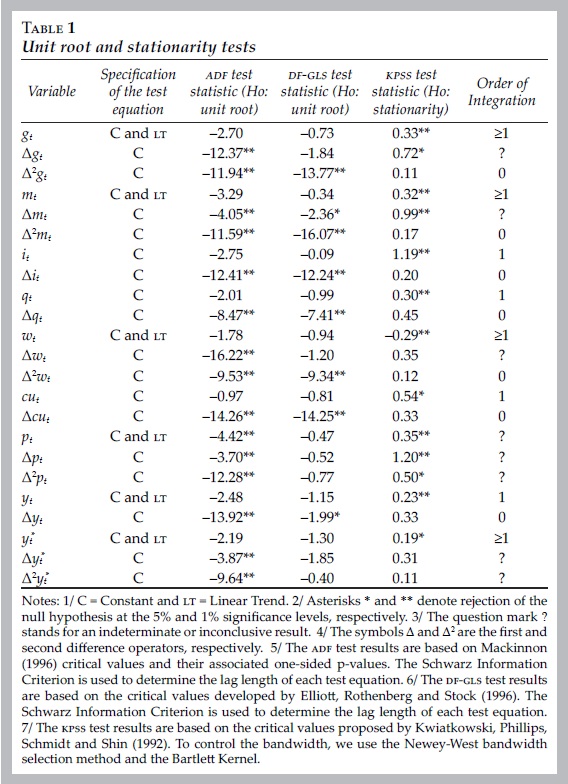
It is worth noting that, in the ADF and DF-GLS tests, the null hypothesis of a unit root is contrasted against the alternative hypothesis of stationarity. On the other hand, in the KPSS tests, the null hypothesis of stationarity is contrasted against the alternative of non-stationarity. The rationale for including a stationarity test, such as the KPSS test, is that the non-rejection of a unit root hypothesis might be due to the lack of power of the ADF and DF-GLS tests. The DF-GLS test, however, has proven more powerful than the ADF test when the test equation includes a constant and a linear trend. Table 1 reports that four variables (i_t, q , cu_t, y_t) are non-stationary in levels and stationary in first differences, so that they can be regarded as The remaining five variables (g_t, m_t, w_t,p_t, y_t*) could in principle involve a higher order of integration, given that the test results are somewhat ambiguous. The second differences of government spending, money supply and nominal earnings (Δ²g_t, Δ²m_t, Δ²w_t) are clearly stationary, but the results are inconclusive in first differences. For instance, the two unit root hypotheses are rejected for the first difference of the monetary aggregate (Δm_t) but the stationarity hypothesis is also rejected. These mixed results also apply to the price level and foreign output, even after differentiating once and twice. Garcés (2002) and Galindo and Catalán (2004), interdict, encounter exactly the same problem with the price level and the monetary aggregates of the Mexican economy, even though the sample period and the tests used differ. Based on previous evidence indicating that the Mexican prices are I(1) in larger samples, Garcés (2002) chooses to treat both money and prices as On the other hand, Galindo and Catalán (2004) work with those series in levels and first differences only, thus treating them as I(1).¹⁶ Moreover, the American industrial production index also seems to be I(1). Hence, it seems reasonable to treat money, prices and the rest of the variables as in levels and I(0) in first differences.

Cointegration analysis

Following the Johansen methodology, we first proceed to estimate an unrestricted and congruent VAR model in nine variables:

where Y_t is an 9x1 vector of variables, X_t is a 2x1 vector of deterministic trends,¹⁷ and η_t is an 9x1 vector of innovations. On the other hand, A_i and ψ are coefficient matrices with dimensions 9x9 and 9x2, respectively.

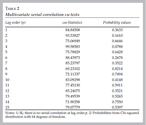
The value of p, that is, the lag length of the VAR model was determined empirically, since the use of different lag length criteria failed to achieve congruency (that is, failed to produce relatively well-behaved residuals). Along these lines, a VAR model with six lags for each variable in each equation is congruent and retains a large enough number of degrees of freedom to efficiently estimate the parameters of the model. Table 2 reports the outcome of the multivariate serial correlation Lagrange Multiplier (LM) tests. The LM statistics and p-values suggest the absence of serial correlation up to lag order fifteen.¹⁸ By the same token, we performed the multivariate version of the White Heteroskedasticity test, revealing that at the 5% significance level the null hypothesis of homoscedasticity cannot be rejected in any of the cases.¹⁹

Despite these encouraging results, in a six-lag VAR most series exhibit residuals with an important number of statistically significant outliers. Consequently, a battery of VAR residual normality tests leads to concluding non-normality and the problem remains despite the addition of more lags.²⁰ Nonetheless, Johansen (1995, p. 20) relaxes the normality requirement in this particular instance, stating that residuals should not substantially depart from Gaussian white noise. Thus, in view of the previous testing, the estimated six-lag VAR model appears to be congruent and suitable for cointegration analysis. Moreover, reducing the information set (that is, the number of variables in the system), increases the number of lags needed to arrive at a statistically well-behaved VAR. Johansen (1995) states that, in some cases, long lags are an indication that the information set of a VAR needs to be broaden.

So, a reparameterisation of equation [8] yields the following expression:

where , and η_t is an i.i.d. vector of innovations with mean zero and variance Ω. Note that the pth order VAR translates into a (p-1)th order vec model. Moreover, the reliability of the empirical evidence in the context of the cointegration analysis requires that η_t be i.i.d. and not n.i.i.d. The fourth implication of the Granger Representation Theorem (Engle and Granger, 1987) states that if a k-dimensional vector of variables is I(1) and involves one or more cointegrating relationships, then there exists a VEC model which can be accurately represented by equation [9]. More specifically, if variables in vector Y_t are I(1) and the rank of the coefficient matrix Π is reduced (r < k), then it can be shown that kxr matrices α and β (both with rank r) exist and are such that: i) Π = αβ' and ii) β'Y_t-1 is stationary. Hence, the columns of β are the cointegrating vectors and β'Y_t-1 contains the r long-run equilibrium relationships among the k variables, where r symbolizes the cointegrating rank. The elements of matrix α are the adjustment coefficients of the VEC model and their values determine the speed at which equilibrium is restored following a shock. The short-run dynamics is also captured by coefficient matrices Γ₁, Γ₂, ..., Γ_(p-1).

Along these lines, VEC models are designed to capture both the long-run equilibrium relationships among the k variables and the short-term dynamic response of each variable to an innovation in another variable. Such a response is also estimated in the context of a k-dimensional model.

As is well known, Johansen's approach essentially lies in estimating equation [9] by maximum likelihood, and then test whether the restrictions derived from the reduced rank of matrix Π can be rejected. So, the main task at this point is to determine the cointegrating rank of Π and estimate both the equilibrium (or long-run) parameters and the adjustment (or short-run) parameters. To that end, we depart from equation [9], which is in principle an unrestricted VAR expressed as a VEC model. The term unrestricted means that no prior restrictions are placed on the rank of Π. The next step, however, is to impose the restrictions associated with the previously depicted model (i.e., the restrictions implied by equations [4], [5], [6] and [7]), given that economic theory should play an important role in determining the number and form of the cointegrating relationships. The objective here is to identify cointegrating equations which are meaningful from an economic viewpoint.

Before performing the cointegration tests, it is necessary to make a plausible assumption regarding intercepts and trends in the cointegrating relationships (or cointegrating space) and the VAR (or data space). Due to the fact that our model is linear, at least in the logarithms of the variables, a constant will be allowed in the cointegrating space such that the long-run equilibrium relations among the variables are not restricted to cross the origin. In addition, given that most level series display a linear trend it was deemed appropriate to include a constant in the data space as well.

To determine the cointegration rank of matrix Π (i.e., to determine the value of r), Johansen proposes two types of likelihood ratio (LR) tests statistics: the trace statistic, denoted λ_trace, and the maximum eigenvalue statistics, denoted λ_max. Although both statistics are LR statistics, they are not asymptotically distributed as a standard Χ² distribution under the null hypothesis. Hence, we will make use of the non-standard critical values developed by Osterwald-Lenum (1992). Johansen's cointegration trace and maximum eigenvalue tests are reported in tables 3 and 4, respectively.

As illustrated in tables 3 and 4, the two tests are used in a sequential fashion, starting at r=0 and ending at r ≤ k-1 until a rejection of the null hypothesis arises. A noteworthy distinction between the trace and the maximum eigenvalue statistics is that the latter stems from a more restrictive alternative hypothesis, which is meant to increase the power of the test.²¹ The trace tests indicate that there are seven (six) cointegrating equations at the 5% (1%) significance level. In contrast, the maximum eigenvalue tests indicate that there are three (two) cointegrating equations at the 5% (1%) significance level.²² After performing the appropriate normalizations, the above discrepancy was resolved in favor of the maximum eigenvalue tests, given that only three vectors were relatively consistent with economic theory. These vectors are presented in table 5 and some of the wrongly signed parameters are fixed subsequently through the application of likelihood ratio tests and the eradication of potentially redundant variables.

In order to convey a straightforward interpretation, we can rewrite the longrun equilibrium relationships as:

In accordance with standard economic theory, equation [10] reports positive coefficients for government spending and foreign output, and a negative coefficient for the nominal interest rate and the price level. Nonetheless, the parameter estimates corresponding to the real exchange rate and capacity utilization are negative. As noted earlier, the net effect of a given currency depreciation seems to be negative in the Mexican economy. On the other hand, a negative coefficient for capacity utilization is certainly not in line with economic theory but this inconsistency will be eradicated by dropping potentially redundant variables from equation [10].

Parameter signs in equation [11] are all theoretically correct, given that money demand is a decreasing function of the nominal interest rate, the real exchange rate, and foreign output.²³ At the same time, we observe that money demand is an increasing function of government spending, prices, capacity utilization (which is used here as a proxy for domestic output). Note that, in principle, there is no evidence of money demand homogeneity with respect to prices (the price elasticity of money demand is greater than unity). It must be highlighted that, in the long run, the level of capacity utilization appears to exert a strong positive influence on money demand. In any event, this finding would be in agreement with previous expectations given that the closer actual output is to potential output, the more money economic agents demand to fulfill their dealings.

In the wage equation (equation [12]), only one parameter sign —the one associated with foreign output— is in principle contrary to our expectations. This problem, however, is resolved by finding a more plausible specification for equation [12]. Consequently, the next step is to determine whether equations [10], [11] and [12] are consistent with our ex ante assumptions regarding the functional form of the is equation (equation [4]), the LM or money demand equation (equation [5]), and the wage-setting equation (equation [6]). In other words, we will test the following three hypotheses by means of likelihood ratio tests:

H^1₀: All parameters in [10] not included in [4] equal zero.

H^2₀: All parameters in [11] not included in [5] equal zero.

H^3₀: All parameters in [12] not included in [6] equal zero.

The probability values associated with the first, second and third null hypotheses are 0.349, 0.378 and 0.000, respectively. Thus, at the 5% significance level, the LR tests lead to the non-rejection of H^1₀ and H^2₀, and to the rejection of H^3₀. Further testing suggests that the only variable that can be dropped from the wage equation is the price level. This amounts to an empirical validation of the is and the money demand equations (equations [4] and [5]), although in the case of the latter capacity utilization had to be used as a proxy for output.²⁴ Finally, the hypothesis that the price elasticity of money demand equals one (i.e., the hypothesis that b₂ in equation [5] equals 1) is rejected at the 5% significance level. In consequence, our VEC model will contain the next three re-estimated error-correction terms (ECT) in each equation:

ECT1_t, ECT2_t and ECT3_t represent the long-run equilibria in the goods, money and labor markets.²⁵ First of all, ECT1_t suggests that, in the long-run, the domestic output is an increasing function of government spending and the level of foreign output, and a decreasing function of the interest rate and the real exchange rate. It is worth mentioning that this relationship remains basically unchanged after replacing the real exchange rate (q_t) for the nominal exchange rate (e_t).²⁶ Secondly, ECT2_t shows, among other things, that a monetary expansion not completely accommodated by a higher output (i.e., by a higher capacity utilization) causes an excess demand for goods and a growing price level, which will gradually restore the equilibrium in the money market. Thirdly, ECT3_t implies that nominal wages respond negatively to the real exchange rate, and positively to government purchases, inflationary expectations (which are mirrored here by the nominal interest rate) and capacity utilization. The intuition behind is that real exchange rate depreciation increases the cost of foreign inputs to domestic firms, thereby reducing economic activity and wages. On the other hand, an improvement in capacity utilization will raise labor demand and, therefore, nominal wages and earnings. In spite of the heavy regulations in the Mexican labor market, the rest of the evidence presented in this paper is consistent with the implications of ECT3_t.

Broadly speaking, shocks cause variables to depart from long-run equilibria (i.e., the error-correction terms differ from zero). Such departures, in turn, trigger a dynamic process through which equilibria are eventually restored. This dynamic process is described by the 9x3 matrix of estimated adjustment coefficients in table 6.

As illustrated above, the short-run behavior of output is significantly influenced by departures from long-run behavior of aggregate demand and wages. By the same token, the short-run dynamics of prices and capacity utilization is responsive to deviations from long-run equilibria of aggregate demand, money demand and wages. The rest of the variables are affected by at least one of the error-correction terms (ECTS), with the exception of government spending and foreign output. Since these particular variables do not seem to adjust to any lagged disequilibria, they should be treated as exogenous (or weakly exogenous, in the Johansen terminology) for the relevant parameters α and β. In this context, following Johansen standard procedure, we shall model a seven-equation system to perform impulse response and variance decomposition analyses.

Sensitivity analysis

The next step is to estimate the dynamic response of each variable to an unexpected change in another variable, in the context of a VEC model. This task will be accomplished by means of generalized impulse response functions, which do not depend on the VAR ordering (see Pesaran and Shin, 1998). Graphs 1, 2 and 3, respectively, depict the 24-month responses of prices, output and earnings to different sorts of shocks. Broadly speaking, a shock can be defined as an unexpected increase in a given variable, whose size is one standard deviation and whose duration is one month. For simplicity, we shall only present those impulse responses that convey some relevant economic meaning.

Graph 1 indicates that monetary, exchange rate and interest rate shocks have positive and long-lived effects on the price level. On the other hand, shocks to the price level itself (i.e., own-shocks) generate a large inflationary effect, suggesting the presence of a strong predetermined component (that is, a high degree of inflationary inertia). Moreover, in the long run, the supply of money appears to be a prominent source of inflation and this finding is consistent not only with the cointegration analysis (see equation [14] and its economic interpretation), but also with the generalized variance decompositions reported in table 7. Real exchange rate depreciation and sudden escalations in the expected inflation rate (as proxied by the nominal interest rate) seem to exert a notable influence on prices as well. The responsiveness of prices to real currency depreciation, however, tends to diminish as the Mexican economy moves from a high-inflation to low-inflation state.²⁷ Lastly, there is no evidence of wages affecting inflation.

In graph 2 we get an idea about the responsiveness of output to three types of shocks. Monetary shocks appear to increase output initially but this effect dies down after a few months and, as we shall see, variance decompositions do not really support this particular finding. Of course, a necessary —but not a sufficient— condition for a monetary expansion to bring about a production gain is that there be enough slack in capacity utilization. Shocks to capacity utilization raise economic activity at impact and this positive effect is persistent overtime. And a shock to wages (i.e., an increase in nominal earnings) discourages economic activity for several months.²⁸

Finally, graph 3 shows that nominal earnings (and, of course, nominal wages) react positively to increases in the nominal interest rate and capacity utilization. This finding is consistent with equation [15], which places the wage variable as an increasing function of nominal interest rates and capacity utilization. Therefore, both labor demand (as measured by capacity utilization) and inflationary expectations (as measured by the nominal rate of interest) display positive effects on nominal earnings. Now, the finding that nominal wages positively react to inflationary expectations and, at the same time, economic activity negatively reacts to wage-shocks is consistent with the wage-price mechanism developed by Tobin (1972).²⁹

The last step is to estimate the generalized variance decompositions (GVDS) for the variables of interest, namely, prices, output and wages. Generally speaking, what we are doing here is decomposing the forecast error of a given variable over different time horizons (i.e., 12 and 24 months) into the components attributable to innovations (or shocks) in all the variables considered. In table 7, we can observe that variance decompositions are for the most part consistent with the empirical evidence provided earlier.

First, let us examine the variance decomposition (VD) for the price level, which is presented at the top of the table. Notice that, after 24 months, the so-called own-shocks (i.e., shocks to pt) account for 33.17% of the price variability, confirming the presence of inertial inflation. Monetary shocks are in second place, being responsible for 28.8% of the variations in the price level. Interest rate and exchange rate shocks explain 12.46 and 8.04%, respectively, of the volatility in prices. The same ranking for the inflationary determinants can be established through visual inspection of graph 1.

The VD for output tells an interesting story as well. After 24 months, we can attribute 45.79 and 34.58 per cent of output variations to own-shocks (i.e., shocks to y_t) and capacity utilization shocks, respectively. Thus, albeit its strong predetermined component, output is largely influenced by the level of capacity utilization. Note that variance decompositions (VDS) and impulse response functions (IRFS) point toward the same conclusion in this respect. Moreover, 24 months ahead, shocks to nominal earnings explain 10.65% of output variations. So, once again, IRFS and VDS are in agreement and can be brought together to assert that earnings shocks (or even wage shocks) discourage economic activity for several months. Finally, VDS suggest that the impact of monetary shocks on economic activity is negligible.

The VD for nominal earnings suggests that the predetermined component ascribed to this variable is strong, but not as much as in the two previous cases. In accord with the cointegration and the impulse response analyses, VDS show that shocks to interest rates and capacity utilization play major roles in accounting for the variability of nominal earnings. In the 12-month forecast horizon, unexpected changes in interest rates explain almost 10% of the variations in nominal earnings. Capacity utilization shocks, on the other hand, can be credited with 19.39% of earnings' volatility 24 months into the future. In the same time horizon, shocks to the real exchange rate account for 18.98% of earnings' variations. Therefore, taken as a whole, the empirical evidence shows that nominal earnings (and, by implication, nominal wages) are an increasing function of the nominal rate of interest and the level of capacity utilization. There is also basis to infer that real exchange rate depreciation is likely to reduce earnings.

 

Conclusions

Generally speaking, the evidence presented suggests that monetary shocks are a major source of inflation, but not of output fluctuations. In the short run, generalized IRFS and VDS show that unexpected changes in money supply do affect the price level. In the long run, the cointegration analysis indicates that a monetary expansion not fully accommodated by a higher economic activity will cause an excess demand for goods and an increasing price level, which will ultimately restore the equilibrium in the money market. Therefore, our finding is consistent with the view that monetary expansions will rapidly bring about more inflation with a minor short-term production gain. In this context, even a risk-neutral policymaker would probably be unwilling to use monetary policy to influence output and the unemployment rate in the long run.

Real exchange rate depreciation raises prices in the short run and appears to discourage economic activity in the long run. According to the sensitivity analysis (based on IRFS and VDS), real currency depreciation exerts a moderate influence on prices and a negligible influence on economic activity. As noted earlier, the Mexican transition from a high-inflation to a low-inflation scenario has probably played a key role in weakening the stagflationary effects of exchange rate shocks. In the long run, however, the cointegration analysis reveals that an undervalued currency may slow down economic activity. Hence, a coherent policy package designed to improve productive capacity and efficiency, both in the export-market-oriented sector and the import-substituting sector, is far more likely to raise net exports and economic growth than exchange rate adjustments alone.

Notwithstanding the current price stability and the well-functioning floating exchange rate system, we find that sufficiently large currency depreciations may accelerate inflation and cause the central bank to miss its target range. In view of this evidence, exchange rate policymakers should make every effort to reconcile the stability required to keep the rate of inflation within its target range, with the flexibility needed to cope with external shocks and sustain international competitiveness. Further research is needed, however, to determine the supply and demand channels through which real currency depreciation affects output and prices. It is also important to study the role played by external shocks as a source of output and exchange rate fluctuations.

The empirical evidence also shows some degree of inflationary inertia. On the other hand, unrestrained inflationary expectations may reduce the predictability of the actual inflation rate and make it difficult for the central bank to restore stability. Increases in nominal earnings, on the other hand, notably discourage economic activity but do not really seem to affect the price level. In this particular case, we actually concur with Arias and Guerrero (1988), who find no evidence of wages affecting prices.

Finally, both cointegration and impulse response analyses are consistent with the view that nominal wages are a positive function of capacity utilization and expected inflation. Consequently, sustaining and even strengthening credibility (particularly among wage bargainers) is of the uppermost importance for the Mexican central bank to keep inflation expectations in line with inflation targets and, in this manner, prevent potential unemployment costs associated with the pursuit of price stability. Put briefly, a lower-than-expected inflation rate will probably increase real wages, reduce output and exacerbate unemployment. Caution must be exercised, however, in interpreting the relationship between inflationary expectations, nominal wages and prices. Although inflationary expectations seem to influence both nominal wages and prices, nominal wages do not really seem to affect the price level. Thus, subsequent research could try to explore how changes in the expected inflation rate pass through to prices.

 

References

Agénor, P. and A. Hoffmaister, "Money, Wages and Inflation in Middle-income Developing Countries", International Monetary Fund (IMF) Working Paper no. 174, 1997, pp. 1-38.         [ Links ]

Arias, L. and V. Guerrero, "Un estudio econométrico de la inflación en México de 1970 a 1987", México, Dirección de Investigación Económica, Banco de México, Documento de Investigación 65, 1988, pp. 1-76.         [ Links ]

Bailliu, H., D. Garcés, M. Kruger and M. Messmacher, "Explicación y predicción de la inflación en mercados emergentes: el caso de México", México, Dirección General de Investigación Económica, Banco de México, Documento de Investigación 3, 2003, pp. 1-33.         [ Links ]

Banco de México, Statistical Series, <http://www.banxico.org.mx>         [ Links ].

Baqueiro, A., A. Díaz de León and A. Torres, "¿Temor a la flotación o a la inflación? La importancia del traspaso del tipo de cambio a los precios", México, Dirección General de Investigación Económica, Banco de México, Documento de Investigación 2, 2003, pp. 1-26.         [ Links ]

Barbone, L. and F. Rivera-Batiz, "Foreign Capital and the Contractionary Impact of Currency Devaluation, with an Application to Jamaica", Journal of Development Economics, vol. 26, 1987, pp. 1-15.         [ Links ]

Bruno, M., "Stabilization and Stagflation in a Semi-industrialized Economy", in R. Dornbusch and J. Frankel (eds.), International Economic Policy, Baltimore, MD., John Hopkins University Press, 1979.         [ Links ]

Cooper, R., "Currency Devaluation in Developing Countries", Essays in International Finance 86, Princeton, New Jersey, Princeton University, (International Finance Section), 1971.         [ Links ]

Cuevas, V., "Efectos de la volatilidad cambiaria en la economía mexicana", in A. Sánchez Daza (coord.), Procesos de Integración Económica de México y el Mundo, México, Universidad Autónoma Metropolitana (uam)/Ediciones y Gráficos eón, 2005, pp. 263-301.         [ Links ]

Díaz-Alejandro, C., "Note on the Impact of Devaluation and Redistributive Effect", Journal of Political Economy, vol. 71, 1963, pp. 577-80.         [ Links ]

Dickey, D. and W Fuller, "Distribution of the Estimators for Autoregressive Time Series with a Unit Root", Journal of the American Statistical Association, no. 74, 1979, pp. 427-431.         [ Links ]

Dickey, D. and W Fuller, "Likelihood Ratio Statistics for Autoregressive Time Series with a Unit Root", Econometrica, vol. 49, 1981.         [ Links ]

Dickey , D., W Bell and R. Miller, "Unit Roots in Time Series Models: Tests and Implications", The American Statistician, vol. 40, 1986, pp. 12-26.         [ Links ]

Dornbusch, R., F. Sturzenegger and H. Wolf, "Extreme Inflation: Dynamics and Stabilization", Brookings Papers on Economic Activity 2, 1990, pp. 1-64.         [ Links ]

Elliott, G., T. Rothenberg and J. Stock, "Efficient Tests for an Autoregressive Unit Root", Econometrica, no. 64, 1996, pp. 813-836.         [ Links ]

Engle, R. and C. Granger, "Co-integration and Error Correction: Representation, Estimation, and Testing", Econometrica, no. 55, 1987, pp. 251-276.         [ Links ]

Galindo, L. and H. Catalán, "Los efectos de la política monetaria en el producto y los precios en México: un análisis econométrico", Economía, Sociedad y Territorio, Dossier especial, 2004, pp. 65-101.         [ Links ]

Garcés, D., "Determinación del nivel de precios y la dinámica inflacionaria en México", México, Dirección General de Investigación Económica, Banco de México, Documento de Investigación 7, 1999, pp. 1-38.         [ Links ]

----------, "Agregados monetarios, inflación y actividad económica en México", México, Dirección General de Investigación Económica, Banco de México, Documento de Investigación 7, 2002, pp. 1-31.         [ Links ]

Goldfajn, I. and S. da Costa, "Exchange Rate Pass-through in Brazil: A Panel Study", Brasil, Banco Central de Brasil, Documento de Trabajo 5, 2000, pp. 1-39.         [ Links ]

Hamilton, J., Time Series Analysis, Princeton, New Jersey, Princeton University Press, 1994.         [ Links ]

Hirschman, A., "Devaluation and Trade Balance: A Note," Review of Economics and Statistics, vol. 31, 1949, pp. 50-53. Instituto Nacional de Estadística, Geografía e Informática (INEGI), <http://www.inegi.gob.mx>         [ Links ].

International Monetary Fund (IMF), International Financial Statistics, <http://www.imfstatistics.org/imf/logon.aspx>         [ Links ].

Johansen, S., Likelihood-based Inference in Cointegrated Vector Autoregressive Models, Oxford, Oxford University Press, 1995.         [ Links ]

Kamas, L., "Monetary Policy and Inflation under the Crawling Peg: Some Evidence from vars for Colombia", Journal of Development Economics, vol. 46, 1995, pp. 145-161.         [ Links ]

Krugman, P. and L. Taylor, "Contractionary Effects of Devaluation", Journal of International Economics, no. 8, 1978, pp. 445-456.         [ Links ]

Kwiatkowski, D., P. Phillips, P. Schmidt and Y. Shin, "Testing the Null Hypothesis of Stationary Against the Alternative of a Unit Root", Journal of Econometrics, no. 54, 1992, pp. 159-178.         [ Links ]

MacKinnon, J., "Numerical Distribution Functions for Unit Root and Cointegration Tests", Journal of Applied Econometrics, no. 11, 1996, pp. 601-618.         [ Links ]

McCarthy, J., "Pass-through of Exchange and Import Prices to Domestic Inflation in some Industrialized Economies", Bank for International Settlements Working Paper no. 79, 1999.         [ Links ]

Montiel, P., "Empirical Analysis of High-inflation Episodes in Argentina, Brazil and Israel", IMF Staff Papers no. 36, 1989, pp. 527-549.         [ Links ]

Osterwald-Lenum, M., "A Note with Quantiles of the Asymptotic Distribution of the Maximum Likelihood Cointegration Rank Test Statistics", Oxford Bulletin of Economics and Statistics, no. 54, 1992, pp. 461-472.         [ Links ]

Patterson, K., An Introduction to Applied Econometrics: A Time Series Approach, London, MacMillan Press ltd, 2000.         [ Links ]

Pérez-López, A., "Un estudio econométrico sobre la inflación en México", México, Dirección de Investigación Económica, Banco de México, Documento de Investigación 4, 1996, pp. 1-49.         [ Links ]

Pesaran, M. and Y Shin, "Impulse response analysis in linear multivariate models", Economic Letters, no. 58, 1998, pp. 165-193.         [ Links ]

Tobin, J., "Wealth, Liquidity and the Propensity to Consume", in B. Strumple, J. Morgan and E. Zahn (eds.), Human Behavior in Economic Affairs; Essays in Honor of George Katona, Amsterdan, Elsevier, 1972.         [ Links ]

Van Wijnbergen, S., "Exchange Rate Management and Stabilization Policies in Developing Countries," Journal of Development Economics, no. 23, 1989, pp. 227-247.         [ Links ]

Wang, P. and J. Rogers, "Output, Inflation, and Stabilization in a Small Open Economy: Evidence from Mexico," Journal of Development Economics, vol. 46, 1994, 271-293.         [ Links ]

Yacamán, J. "Un análisis de la inflación en México", México, Dirección de Investigación Económica, Banco de México, Documento de Investigación 48, 1982, pp. 1-20.         [ Links ]

 

Notas

I am grateful to two anonymous referees for their valuable suggestions and comments. All remaining errors are my own.

¹ Most empirical studies try to gather evidence consistent with a particular theory, thereby focusing on a specific set of variable.

² From January 2003 on, the Mexican central bank has officially set a long-term point target of 3% for the annual inflation rate, with a symmetric range of +/-1 percentage point. The target range constitutes a realistic margin of error, in view of the volatility of the National Consumer Price Index and the country's traditional vulnerability to exogenous shocks.

³ As we shall argue, the Mexican transition from a high-inflation to a low-inflation scenario has probably lessened the importance of the exchange rate as a source of macroeconomic fluctuations.

⁴ Montiel (1989) provides similar evidence for Argentina and Brazil using the VAR technique. He finds that, even though money and exchange rate shocks are both important sources of inflation in these two countries, the exchange rate clearly became the most important inflationary force as inflation accelerated during the 1980s. Subsequent research, as we shall see, corroborates the notion that the higher the inflation rate is, the more responsive local prices are to external sources of inflation.

⁵ Kamas (1995) reaches a similar conclusion for the Colombian economy. She uses domestic credit as the variable that reflects the status of monetary policy and proves, within a VAR framework, that an unexpected monetary expansion produces a negligible effect on output.

⁶ Therefore, regarding the wage-effect on inflation in Mexico, Agenor and Hoffmaister (1997) contradict Arias and Guerrero (1988), who find no evidence of inflationary pressure stemming from wage increases, and go farther than Yacaman (1982), who makes only reference to a short-term impact on prices. This discrepancy probably reflects the sensitivity of the empirical evidence with respect to two basic choices: the period under examination and the length of the period. Perez-Lopez (1996), for instance, notes that between 1989 and early 1994 the variation rate in wages exceeded the variation rate in inflation which, at the same time, was higher than the variation rate in foreign prices (expressed in local currency). From late 1994 on, the above situation reversed; that is, the local-currency value of foreign prices began to exhibit the highest variation and wages the lowest, with inflation variation lying somewhere in between. Consequently, the relative contribution of a given variable to the inflation rate may depend on the choice and scope of the sample period.

⁷ Of course, the rate of inflation is not the only determinant of the magnitude of the pass-through effect. According to McCarthy (1999), the size of the pass-through effect and the degree of openness of an economy are positively correlated. Furthermore, based on a panel study including 71 countries, Goldfajn and da Costa (2000) show that the extent of the pass-through effect depends not only on the degree of openness of the economy and the rate of inflation itself, but also on the cyclical component of output and the initial overvaluation of the currency.

⁸ The choice of the nominal interest rate, as opposed to the real interest rate, is based on the Johansen methodology which requires all variables to be nonstationary in order to perform cointegration tests and estimate a VEC model.

⁹ As is well known, the log of the real exchange rate, q_t, can be written as: q_t = s_t + p_t*-p_t, where s_t is the log of the nominal exchange rate, p_t* is the log of foreign prices, and p_t is the log of the domestic price level. Thus, q_t is the logarithmic version of the relative price of imports in terms of domestic goods.

¹⁰ The disturbance term ε_t^w can also serve to mirror sudden changes in the size of the informal sector, the degree of labor mobility, the government labor policy, and the bargaining power of unions versus firms.

¹¹ The Fisher equation states that: i_t= r^e_t + π^e_t, where r^e_t is the expected real interest rate and π^e_t is the expected inflation rate at time t.

¹² Use of the actual unemployment rate was discarded, as this variable appears to be stationary and cannot be part of the cointegration tests. The output gap, estimated through the Hodrick-Prescott filter, also proved to be stationary in levels. As we shall see, the capacity utilization index is in levels and can thus be included in the cointegration analysis.

¹³ Assuming that the domestic price level is downwardly inflexible, real exchange rate depreciation could arise from nominal exchange rate depreciation and/or from inflation abroad. In any event, foreign inputs will become more costly to domestic firms and there will be more pressure on the domestic price level.

¹⁴ Source: Instituto Nacional de Estadística, Geografía e Informática (INEGI), Banco de México, and International Monetary Fund (IMF).

¹⁵ The null hypothesis of a unit root with no deterministic trend was tested against the alternative hypothesis, which included a deterministic trend.

¹⁶ They argue further that these variables are non-stationary in levels regardless of possible structural breaks.

¹⁷ As we shall see later, X_t contains a 1, which captures the intercept term in each equation, and a time trend t.

¹⁸ We also estimated the matrix of pairwise cross-correlograms —with two-standard error bounds— for the VAR residuals, which are broadly consistent with the absence of autocorrelations.

¹⁹ For the sake of brevity, this test results are available upon request.

²⁰ Results of these tests are also available upon petition.

²¹ See Patterson (2000, pp. 620-621) for a detailed discussion on the subject.

²² A key issue is whether, and to what extent, the test results are sensitive to the underlying assumptions made about trends and intercepts in the cointegration space and the data space. To deal with this matter we performed a battery of cointegration tests under different specifications for deterministic terms. The main finding was that the maximum eigenvalue tests reported exactly the same outcome, even with implausible specifications. Besides, the cointegrating equations with the baseline specification (i.e., with a constant in the cointegration space and a linear trend in the data space) were graphed against time. The result was that those equations enclose the horizontal axis for an extended period of time, thereby showing that no linear trend needed to be accounted for in the cointegrating space.

²³ Real currency depreciation is consistent with a lower demand for domestic currency. By the same token, an increasing output abroad might strengthen the demand for American dollars and weaken the demand for Mexican pesos.

²⁴ Use of actual output in the money demand equation gives rise to inadequate results for the other two cointegrating equations.

²⁵ In this manner, we have two cointegrating relations stemming from the demand side of the economy (equations [13] and [14]) and one from the supply side (equation [15]).

²⁶ In this particular case, the resulting error-correction term is: ECT1_t = -y_t + 2.263 + 0.188g_t - 0.0051i_t- 0.218e_t + 0.006y_t*.

²⁷ In fact, when we extend the sample period backward to include the December-of-1994 devaluation of the peso and its aftermath, we find that the pass-through effect from the real exchange rate to the price level increases. This finding is consistent with the empirical study conducted by Baqueiro, Díaz de León, and Torres (2003).

²⁸ We believe that this effect would have to subside after some time, but we are unable to show it because our impulse responses do not include confidence intervals.

²⁹ This model consists of a price (or markup) equation and a wage equation. The markup equation depicts the behavior of prices and could be regarded as an inverse supply curve. The wage equation, on the other hand, is the Phillips curve. One important feature of this framework is nominal-wage stickiness, so that nominal wages respond to changes in expected inflation but have a delayed or partial response to unanticipated inflation. Thus, an unanticipated increase (decrease) in inflation reduces (raises) real wages which, in turn, has a transitory positive (negative) effect on economic growth.