Introduction

^{Pasinetti (2000)} has developed a thorough critique of the distribution theory that underlies neoclassical growth theory. ^{Rada and Taylor (2006)} have concluded that such theory is empty of content, since it rests on the flawed neoclassical production function. They argue, however, that the latter theory can be fruitfully substituted by productivity equations models derived from national accounts conventions and algebraic identities. They point out that these models, based on identities, are bound to fit empirical data. Models constructed on national accounts identities, when applied to empirical data, will uncover long term structural tendencies and breakpoints of specific capitalist economies.

Two growth models, put forward by Gérard Duménil and Dominique Lévy and by Duncan Foley and Thomas Michl, are discussed below. Each belongs to the type of aggregated macroeconomic models derived from national account identities and to the Classical economic tradition. I believe that these models represent a powerful approach to explaining historical and current economic tendencies in real economies such as the economies of Latin America. Nevertheless, they reproduce the limitations and omissions of aggregate analysis, and some constraints derived from their specific assumptions. Moreover, there are empirical difficulties that stem from the design and availability of national accounts data.

The aim of Duménil and Lévy and Foley and Michl is to formalize the long-term tendencies of capitalist economies proposed by Karl Marx in Capital. ^{Duménil and Lévy (2003)} have called these tendencies “trajectories à la Marx,” while ^{Foley and Michl (1999)} have labeled their model a “Classical model of growth with Marx-biased technical change and constant wage share.” For these authors, during long periods, but not indefinitely, developed capitalist economies are subject to trajectories à la Marx. Some of the patterns of these trajectories do coincide with the stylized facts proposed by Nicholas Kaldor, but others, such as the constancy of the output-capital ratio, do not (see for example ^{Kaldor, 1957}).

Duménil and Lévy’s and Foley and Michl’s models are quite similar. Each assumes a capitalist economy with two classes (capitalists and workers), which produces only one good. Duménil and Lévy offer theories of real wage and technical change. Foley and Michl postulate that the real wage grows at the same rate as labor productivity and that both labor productivity and the output-capital ratio (the technical variables) evolve at given growth rates. I am interested here in presenting the patterns of growth derived from these models to analyze the economic growth behavior of Latin American economies in comparison with that of the United States (US). I will not discuss Duménil and Lévy’s specific growth functions, nor their wage and technological change theories (^{Duménil and Lévy, 1995}, contains a detailed discussion of their technological change model). Moreover, a discussion of economic policies in Latin America is beyond the scope of this paper.

The paper is organized as follows. The first two sections develop in detail the models of Duménil and Lévy and Foley and Michl. The next section presents an empirical test of Neoclassical versus Classical economics designed by Foley and Michl. Then several theoretical caveats, some applicable to all aggregate macroeconomic growth models, others specific to the chosen models are discussed. Next country selection, the database, and the methodology for construction of variables are explained, along with some remarks on the quality of the database. After that, an analysis, based on the theoretical models presented in previous sections, of economic growth patterns in Argentina, Brazil, Chile, Colombia, Mexico, and the US is offered. Finally, summary and concluding remarks appear in the last section.

Duménil and Lévy model

According to ^{Duménil and Lévy (2003)}, in Marx there are three long-term tendencies at work in a capitalist economy: the growth of labor productivity, the increase of the value composition of capital, and the fall of the profit rate (though the mass of profits can be growing). These tendencies are counteracted or nullified by rises in the rate of surplus value and by increases in the share of profits accumulated in relation to the total profits (rate of accumulation). Below we will formally define these categories.

For ^{Duménil and Lévy (2003)}, the variables that determine the path of a capitalist economy interact with each other: given the real wage and the existing technology (a set of techniques of production), capitalists can compute the profit rate of each technique. They then choose the more profitable technique. Thus, the real wage indirectly determines the technique in use and the profit rate, which in turn determines the rate of accumulation. Then, depending upon the technique in use, the rate of accumulation sets the level of output and employment. Finally, the employment level affects the real wage. The theories of technical change and real wage are crucial in Duménil and Lévy. In particular, if the technical change that prevails is one that raises the composition of capital, the output-to-capital ratio (or capital productivity) tends to decrease. Therefore, though a positive rate of accumulation increases the stock of capital, it becomes less productive, due to the type of technical change that is taking place.

Following ^{Duménil and Lévy (2003)}, and adopting Foley and Michl’s notation, let us define Y, K and N respectively as net output, fixed capital (in same monetary units than output), and number of workers employed. The technical parameters are given by y = Y/N (net output per worker or net labor productivity) and φ = Y/K (net output-to-capital ratio or net capital productivity). w is the real wage per worker, and W = wN is the total wage bill. Let us define R as the net profit, ψ as the wage share in net output and θ as the profit share in net output. Then

[1]

[2]

Marx’s rate of surplus value (R/W), the profit share (θ), and the wage share (ψ) are alternative measures of distribution, since R/W = θ/(1 - θ) = (1 - ψ)/ψ. If one of these variables is constant, the other two are constant. If the wage share increases, the rate of surplus value decreases. The wage share can be expressed as the real wage divided by labor productivity.

[3]

The net profit rate -net profits by unit of capital- is given by r = R/K, and the value composition of capital -capital in monetary units divided by the wage bill- by λ=K/W. Note that the net output-capital ratio and the net profit rate can be written as follows:

[4]

[5]

Therefore, if the wage share (or the profit share) is constant, by equation [4] the net output-capital ratio will change inversely with changes in the value composition of capital, the wage ratio by equation [3] will move at the same rate as net labor productivity (w = ψy), and the profit rate by equation [5] will change at the same rate as the net output-capital ratio (r = θφ).

A trajectory à la Marx implies that the net output-capital ratio and the profit rate will fall while labor productivity and the real wage will rise. In equation [5] with a net profit share held constant, a falling net output-capital ratio reduces the profit rate. Let us define g _x as the annual growth rate of variable x. The annual growth rate of capital is given by the Cambridge equation; that is to say, it is equal to the share of net profits that goes to capital accumulation (or rate of accumulation), s _R , times the net profit rate:

[6]

If the profit rate is falling, the growth rate of capital will fall if the share of net profits that goes to capital accumulation is constant or is falling. As long as net capital productivity falls and net labor productivity raises, the annual growth rates of net output and employment will also fall, even faster than g _K , since

[7]

[8]

Duménil and Lévy show, through special time functions, that with a constant wage share, it is possible to have trajectories à la Marx that do not end in stagnation. The rate of profit falls, while capital, profits, accumulated profits, output and employment all rise, though at a decreasing rate of growth. Without these functions, the model achieves a point in which the economy comes to a halt -as occurs in Foley and Michl’s model.

Foley and Michl’s model

In their book Growth and Distribution, Foley and Michl develop several growth models, departing from a common model of production based on Sraffian real wage-profit rate curves. Their seventh chapter is dedicated to a classical growth model with Marx-biased technical change. Labor productivity grows while capital productivity decreases. This model of biased technical change also appears in ^{Foley and Marquetti (1999)}, ^{Foley and Marquetti (2000)}, and ^{Michl (1999)}.

As in Duménil and Lévy’s model, Foley and Michl’s hypothetical economy produces only one good, which is used either for consumption or accumulation. Their economy is closed and does not have a governmental sector. Using their notation, Foley and Michl define gross product and fixed capital stock in monetary units as X and K, respectively, and the number of workers employed as N. Total wage bill and gross profits are defined as W and Z, and consumption and gross investment as C and I, where I is equal to the increase of the capital stock (∆K) plus depreciation (D). Therefore,

[9]

[10]

In Foley and Michl’s work, output, profits, and investment variables are referred to quantities including depreciation. Here, unless explicitly specified, these variables and the relations where they enter are gross of depreciation. Let us define x = X/N as labor productivity, ρ = X/K as the output-capital ratio, and k = K/N as the capital-labor ratio. The profit share in output is given by π = Z /X, the profit rate by v = Z/K = (Z/X)/(K/X) = πρ, the depreciation rate by δ = D/K, and the real wage (wage per worker) by w = W/N. The capital-labor ratio can also be written as k = x/ρ. Finally, g _K = ∆K/K is the rate of growth of the capital stock. Therefore, dividing by the number of workers and rearranging, equations [9] and [10] become:

[11]

[12]

Equation [11] is the schedule (line) real wage-(gross) profit rate, which has a -k slope and extreme points v = 0, w ^max = x, the coordinate (0, x), and v ^max = x/k = ρ, w = 0, the coordinate (ρ, 0); see in Graph 1 lines x ₀ρ₀ and x ₁ρ₁. Equation [12] is the schedule (line) consumption per worker-growth rate, which also has a -k slope, and its extreme points are g _k + δ = 0, c ^max = x, the coordinate (0, x), and (g _k + δ) ^max = x/k = ρ, c = 0, the coordinate (ρ, 0). Since both schedules are mathematically identical, Foley and Michl call their union the growth-distribution schedule. In equations [11] and [12], an inverse (classical) relationship between the real wage and the profit rate and the consumption per worker and the growth rate of capital is present.

Graph 1: Growth-distribution schedule 

Assuming that the depreciation rate is constant through all techniques, a technique of production can be described either by labor productivity and the capital-labor ratio (i.e. by x, k) or by labor productivity and capital productivity (i.e. by x, ρ). Once x and k (or ρ) are known, if a theory of wage determination and a theory of savings are added to equations [11] and [12], the growth model can be solved for the wage rate, the profit rate, the consumption per worker and the growth rate of capital stock. Foley and Michl use a version of the Cambridge equation where one plus the growth rate of capital (the growth factor) is equal to the fraction β used as capital in the current period of the sum of the capital from the previous production process plus net profits (the wealth stock: K + Z - D) divided by the previous capital:

[13]

Assuming that the profit share in output, π, is constant, the real wage, as in equation [3], will grow at the same pace as labor productivity:

[14]

To model technical change, assume that labor productivity grows at the rate γ and capital productivity evolves at the rate χ. These add two equations to the growth model:

[15]

[16]

Equations [11] through [16] form Foley and Michl’s classical growth model. The parameters of the model are x ₀, ρ₀ (or k ₀), δ, β, π, γ, and χ. The endogenous variables are x, ρ (or k), w, v, c, and g _K . Note that if π is constant and ρ decreases at the rate χ, the profit rate declines, because v = πρ (which is equivalent to equation [5], which calculates the net profit rate). Since v - δ is also declining, the rate of growth of the capital stock will also fall by the Cambridge equation, equation [13]. The stock of capital will stop growing altogether when the net profit rate (v - δ) equals (1 - β)/β. The growth rate of output will also fall, since this growth rate is equal to the rate of growth of the capital stock plus the rate of growth of capital productivity:

[17]

If γ > 0 and χ < 0, Marx-biased technical change is taking place (labor productivity increases and capital productivity falls). The growth-distribution schedule shifts to the left in the v, g _K + δ axis, and to the top in the w, c axis, as is shown in line x ₁ρ₁ with respect to line x ₀ρ₀ in Graph 1. Marx-biased technical change implies that there are savings of labor and more consumption of capital per unit of good produced. Alternatively, Marx-biased technical change can be described as an increase in both labor productivity and the capital-labor ratio (i.e. the absolute value of the slope -k rises). If the profit share (π) is constant, the real wage will grow at the same rate as labor productivity, and the profit rate will diminish at the same rate as the output-capital ratio. If Marx’s technical change is at work, a rising real wage will lead capitalists to shift to an available technique of production with higher labor productivity and lower capital productivity than the technique in use, a move that will produce an inevitable fall in the profit rate.

Two other shifts of the growth-distribution schedule are relevant. One is Harrod’s neutral technical change, where labor productivity grows while capital productivity remains constant (i.e. γ > 0, χ = 0). If the profit share is constant, the real wage grows at the same rate of labor productivity and the profit rate does not change. The other is Hicks’ neutral technical change, where both labor productivity and capital productivity rise in the same proportion (i.e. γ = χ > 0). If the profit share is constant, the real wage will increase at the same rate as labor productivity and the profit rate will rise at the same rate as the output-capital ratio.

The general conclusion of the Duménil and Lévy model and Foley and Michl’s is that in a growth model with growing labor productivity and decreasing output-capital ratio, the rate of profit and the rate of growth of the economy will diminish. ^{Eltis (2000)} has shown that in a Marxian growth model, for any initial values, the rate of profit will eventually begin to fall. This will happen if it is postulated that the rate of growth of output is greater than the rate of growth of variable capital (the wage bill) and lower than the rate of growth of constant capital (the capital stock). This result is achieved at the same time that the rate of surplus value is growing. Eltis, however, has emphasized that to put in motion the forces that produce Marx-biased technical change, increase in the real wage is a necessary condition.

An empirical test of neoclassical and classical economics

According to ^{Foley and Michl (1999)}, an innovator’s profitable adoption of biased technical change can occur before the wage rate increases. But ultimately, via class struggle and a composition effect, the whole capitalist class will end up with a lower profit rate. Each capitalist would adopt a new technique, given the real wage, if the transitional profit rate generated by this technique is greater than that generated by the technique in use. Under the assumption of a constant wage share and Marx-biased technical change, when all capitalists employ the new technique, the final profit rate will be lower than that generated by the previous technique. Given the wage rate, Foley and Michl show that capitalists will adopt the new technique, if:

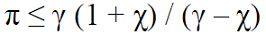[18]

They observe that for Neoclassical economic theory, with a continuum of techniques, this viability condition must hold as a strict equality in order to satisfy the postulate that the wage is equal to the marginal product of labor. Classical economics allows π be equal or less than the right hand side of equation [18]. Therefore, if π < γ(1 + χ)/(γ - χ) for a given economy, then that economy is not working under Neoclassical economics’ assumptions.

With data from twenty-two Organization for Economic Co-operation and Development (OECD) countries from 1965 to 1995, ^{Foley and Michl (1999)} found an overwhelming tendency for π to be less than γ(1 + χ)/(γ - χ). Then developed capitalist economies worked at wage levels above the marginal productivity of labor. ^{Michl (1999)} presents similar results for six developed countries between 1973 and 1992. He found that the right hand side of the viability condition was between 0.52 and 0.72, while profits were one third of income for those countries [note that in ^{Michl (1999)} the viability condition is written as π ≤ γ/(γ - χ)].

In the Neoclassical context, Marx-biased technical change can be viewed as a movement along an isoquant. ^{Zeira (1998)} has recognized the stylized fact that labor productivity tends to grow while capital productivity tends to decrease. For Zeira, the choice of a technique is a standard neoclassical choice along the isoquant, which depends on the relative price of the production factors. A rise in the wage rate relative to the interest rate will generate an increase in labor productivity and a fall in capital productivity. For ^{Michl (1999)}, though the historical data can fit a Cobb-Douglas production function, one cannot assume a continuous and differentiable production function as the viability condition, equation [18], shows.

Theoretical caveats

Both the Duménil-Lévy and the Foley-Michl models, as macroeconomic aggregate models, are subject to at least two critiques. The first one derives from Piero Sraffa’s work. The inverse relationship between the real wage and the profit rate showed in equation [11] and Graph 1 holds for economies with more than one good, but as Sraffa showed, this relationship is no longer linear. Equation [11] is only an approximation of the true real wage-profit rate schedule of economies that produce more than one good. In these economies the phenomenon of technique re-switching appears, i.e. the direct and one to one relation between the level of the wage rate, on the one hand, and labor productivity and capital to labor ratio, on the other hand, does not necessarily hold. ^{Foley and Michl (1999, chapter 3)} and ^{Foley and Marquetti (1999)}, discuss the limits of their economic growth model.

The second critique has to do with the fact that macroeconomic aggregate models cannot take into account the structural changes that are normally at work in a capitalist economy. Technical change increases average incomes, modifies the composition of output and employment, changes the price structure, and transforms demand and consumption patterns (see ^{Pasinetti and Scazzieri, 1987}). In the early stages of economic development, the agricultural sector decreases its share of output in favor of the industrial sector, while in a modern developed economy, the industrial sector itself loses share, and services increase their importance. Therefore, an important composition effect exists behind the changes in both aggregate labor productivity and capital productivity. ^{Kongsamut, et al. (2001)} have underscored these structural changes, which they label Kuznets facts, and attempt to make them compatible with the Kaldor facts within a neoclassical balanced growth model, where the sectors’ shares are changing.

For the Duménil-Lévy and Foley-Michl models, I would argue that at least three limitations should be highlighted. First, the model assumes a closed economy. The presence of an external sector is very important in real economies and for some, such as in Mexico, the weight in gross output of total external transactions should not be disregarded, especially in the expenditure side of the model (i.e. equations [10] and [12] in the Foley-Michl model).

The other limitations are connected with the concept of capital in Marx and with the calculation of the profit rate. On the one hand, the aggregate Duménil-Lévy and Foley-Michl models cannot differentiate between the two categories that form constant capital, in Marx’s terminology: fixed capital (buildings, machinery and equipment) and constant circulating capital (raw and auxiliary materials). Each category has a different turnover time. However, as we will see in the next section, given the way that capital stock, K, is empirically calculated it folds together both types of constant capital. Therefore a crucial point is whether the chosen depreciation rate to calculate K via the perpetual inventory method is really an accurate weighted average of the different kinds of capital stock depreciation rates.

On the other hand, wages are explicitly not included in capital. This implies that workers are paid after production takes place and therefore capitalists do not advance capital to buy labor, which is not the case in real economies. This assumption underestimates the amount of total capital advanced by the capitalists, and increases the profit rate, since K is only composed by constant capital. This problem cannot be solved by adding the wage bill, W, to K, since wages, which are circulating capital, have a specific turnover time, which may be on average different of one year. However, with all these caveats in mind, I believe that the empirical use of these models can shed light on growth tendencies in major Latin American economies, and allows us to compare them with the growth behavior of a developed economy, like the United States economy.

Country selection and database

For this exercise, I selected five major Latin American countries. According to Economic Commission for Latin America and the Caribbean (ECLAC, 2006), these countries concentrate 82 percent of the 2005 gross domestic product (GDP) of Latin America and the Caribbean at constant 2000 dollars. These economies, along with their shares of the Latin America and the Caribbean 2005 GDP, are as follows: Brazil (30.3), Mexico (28.7), Argentina (14.2), Colombia (4.5), and Chile (4.2). I limited the sample to five countries, excluding Venezuela, whose share of the combined GDP of Latin America and the Caribbean is 5.9 percent. This was because Venezuela is the only one of the largest economies whose mining and quarrying sector represents 18 percent of its GDP (the next highest being Chile, at under 7 percent), and also because the oil rent may introduce distortions in its economic performance. The United States is included for the sake of comparison.

Following Adalmir Marquetti’s procedure in his Extended Penn World Tables Version 2.1, EPWT2.1 (^{Marquetti, 2004a}), I recalculated the database for the six selected countries. Marquetti used the Penn World Table Version 6.1, PWT6.1 (in ^{Heston, Summers and Aten, 2002}). I am using the Penn World Table Version 6.2, PWT6.2 (in ^{Heston, Summers and Aten, 2006}) to generate the variables contained in the Foley-Michl growth model, equations [11]-[16] ([12], [13], [14], [15]). For methods of construction of variables in PWT and EPWT, the reader should check the documentation sections in their respective web sites.

All primary variables, except workers share in output, were taken from PWT6.2. They are as follows: population; real GDP per capita (2000 constant international dollars, chain series); investment share of real GDP per capita (2000 constant international dollars, Laspeyres series); and real GDP chain per worker (2000 constant international dollars, chain series), where “Worker […] is usually a census definition based of economically active population.” [See “Data Appendix for a Space-Time System of National Accounts: Penn World Table 6.1 (PWT6.1)” in PWT6.1 documentation].

PWT6.2 contains data for the period 1950-2004 for the countries considered, except for the case of Chile, with data for 1951-2004. The study period is 1963-2003 (1964-2003 for Chile). The number of workers for 2004 cannot be deduced from PWT6.2. The Constant Capital stock variable, K, is calculated using the Perpetual Inventory Method (PIM), with the following formula:

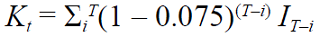
where I is constant gross investment, T = 14 and i = 1, 2,…, 14. See Marquetti’s (2004a) “This dataset was compiled from the Penn World Tables and other sources.” By construction, capital stock series are available for 1963 to 2004 for all the countries, except for Chile, whose capital stock series begin in 1964.

Finally, I took Marquetti’s workers’ share in output, remunerations divided by gross domestic product, in EPWT Version 2.1, which was taken from several issues of the United Nations’, National Accounts Statistics: Main Aggregates and Detailed Tables. I updated this variable with national accounts data from each government’s statistics agency (listed at the end of the bibliography) as follows:

The data set, which is available from the author upon request, contains homogeneous and comparable data of the Foley-Michl growth model variables. In a database with the scope of the EPWT there can be several problems with the quality of the data and the way the variables were constructed. Working with the statistics of only one country in its own monetary unit may allow researchers to avoid the compromises of a database encompassing several economies and to gain accuracy, but it can also preclude comparative analysis of growth performance. ^{Marquetti (2003)} uses EPWT to analyze historical and regional patterns of technical change. For an analysis of Brazil using the Foley-Michl growth model, see ^{Marquetti (2004b)}. Mexico is analyzed in ^{Mendoza (2003)}. The main source for an analysis of the US economy from the perspective of the models presented here are Duménil and Lévy’s papers; see, for example, ^{Duménil and Lévy (2004)}.

There are at least three variables whose construction is perhaps the most problematic: capital stock, K, number of workers, N, and the wage share in output, 1 - π. K includes all net capital, except wages, since it is calculated from total gross investment (fixed gross investment plus inventory changes). Marquetti’s method for estimating the capital stock assumes a uniform depreciation rate of 0.075 for all countries. According to Marquetti, this relatively high depreciation rate underestimates the size of the capital stock and increases the variance of its rate of growth. However, Marquetti assumes that there is not any systematic deviation of these rates of growth. Therefore, because K does not include wages, and because for the included part, it is underestimated, variables in which it enters as divisor will be overestimated (output-to-capital ratio, ρ, profit rate, v).

The number of workers, N, based on the census variable economically active population, encompasses, in the one hand, more than wage earners or productive workers (such as clerks, self-employed, and owners) and, in the other, employed and unemployed people. Therefore, N is likely to overestimate the labor force. In the case of the wage share, as long as there exists, in real economies, aside from capitalists and workers, a group of self-employed whose income is imputed to profits, 1 - π may also be underestimated. ^{Rada and Taylor (2006)} remind us that this problem does not have an easy solution and recount the attempts to solve it by several researchers. One last remark: note that consumption, C, is equal to real GDP less gross investment (C = X - I), and therefore includes the external trade balance.

Behavior of major Latin American countries and the United States, 1963-2003

The economies considered are dissimilar and show different behaviors over time. The absolute value of US labor productivity, x, in 2003 was 67.9 thousand constant 2000 international dollars (see Table 1). In the same year, relative to US, labor productivity was 42.6 percent in Chile, 35.8 in Argentina, 27.4 in Mexico, 22.8 in Brazil, and 20.3 in Colombia. There is a huge labor productivity gap between US and Colombia, but also between Chile and Colombia. The differences in labor productivity (x), the capital-labor ratio (k), and the real wage rate (w), among the five Latin American countries and the US are remarkable.

Table 1: Foley-Michl growth model. Variables evolution by country, 1963-2003 

Notes: * Data for these variables is for the years 1993 and 2003 for Argentina and 1970 and 2003 for Mexico. Mean growth rates were calculated using the available data (see section: Country selection and database). ** Mean value of the variables, i.e. mean growth rates of K and X.

Source: see section: Country selection and database.

Graph 2 plots the evolution of the log of labor productivity for each country. It shows that around 1980 there is a marked change from rapid and relatively stable growth to stagnation, huge backward movements, and high volatility in the cases of Argentina, Brazil, Colombia, and Mexico. In contrast, Chile’s labor productivity behaves inversely: it began with marked cyclical behavior before 1985, and then grew rapidly after that year. The US economy shows a more stable pattern: labor productivity growth is certainly slow during the period, but its falls are short lived and are not deep, the recessions of the mid 1970s and the early 1980s perhaps being the exceptions. Thus, after forty years, labor productivity in Latin American countries has diverged from labor productivity in the US. The percent mean annual growth rates of x in 1963-2003 are: Argentina, 0.8; Brazil, 1.5; Chile, 1.6; Colombia, 1.0; Mexico, 1.0; and US, 1.8.

Source: see section: Country selection and database.

Graph 2: Log of labor productivity by country, 1963-2003 

The output-capital ratio, ρ, also shows a structural breakpoint at the beginning of 1980s in the majority of the countries (see Graph 3). In Argentina, Brazil, and Mexico the relatively long fall of this ratio clearly reverses. In the US (and perhaps in Colombia, but with large swings), where the output-capital ratio was also falling before early 1980s, a certain stabilization occurs. In Argentina, Mexico, and the US, this ratio began to fall again in the mid 1990s. Chile is again the exception, since it presents a growing output-capital ratio through the period 1964-1989 and a falling ratio since 1989.

Source: see section: Country selection and database.

Graph 3: Output-capital ratio by country, 1963-2003 

In Table 1, the period 1963-2003 is subdivided into subperiods of technical change patterns. For each country, a technical change pattern is defined as the segment of time between a trough and a peak, or vice versa, of the output-capital ratio. The technical change pattern is characterized according to the value of the mean annual growth rates of labor productivity (g _x ) and the output-capital ratio (g _ρ). Recall that alternatively a technical change pattern can be characterized by the growth rates of labor productivity (g _x ) and the capital-labor ratio (g _k ), where g _k = g _x - g _ρ. Technical change is defined as Harrod if g _x > 0.0040 and -0.0040 < g _ρ < 0.0040, as Hicks if g _x , g _p > 0.0040, as Marx if g _x > 0.0040 and g _ρ < -0.0040 (Marx), and as crisis if for any value of g _p , g _x < 0.0040.

Subperiods were fairly easy to define for each country, except for Colombia, due to dramatic short-term swings of the output-capital ratio after 1984. Note that in Table 1, aside from the five subperiods of technical change crisis, Marx-biased technical change appears in seven subperiods, followed by Hicks and Harrod with three and two, respectively. Therefore, Marx-biased technical change is not a rarity, and it would be worth analyzing in depth the likely reasons behind this kind of technical change. Taking into account the theoretical relationships in equations [11]-[16], analysis of the evolution of technical and distributive variables can proceed for each country and subperiod.

For the period 1963-2003, Argentina, Brazil and Colombia followed a Harrod neutral growth path. For this period, due to the lack of data, it is not possible to discern distributive variables tendencies for Argentina. For Brazil, the real wage (w) grew more than labor productivity (x), and therefore the wage share (1 - π) increased while the profit rate (v) fell (recall that the growth rate of the profit rate can be written as g _v = g _π + g _ρ). Colombia took the inverse trajectory: the real wage grew less than labor productivity, then the wage share decreased and the profit rate rose.

Mexico and the US followed a Marx-biased technical change in 1963-2003. In both countries, the profit rate fell. In Mexico a stagnant real wage and a falling wage share (data for 1970-2003) did not compensate the fall in the output-capital ratio, and the profit rate decreased. In the US, the real wage grew at a slightly higher rate than labor productivity. Therefore, the wage share saw a small increase, which along with the fall in the output-capital ratio determined the reduction of the profit rate. Finally, in Chile the technical change was of the Hicks type during 1964-2003. The wage rate grew more than labor productivity and the wage share increased, but the strong rise of the output-capital ratio also implied an increase in the profit rate.

For all these Latin American countries except Chile, the final years of the period 1963-2003 were of technical change crisis (stagnant or falling labor productivity) associated with an increase in the output-capital ratio (which reversed in the 1990’s in Argentina and Mexico). In Argentina, after 1994 the fall in labor productivity was very steep and the output-capital ratio began to decrease. These resulted in a simultaneous fall of the real wage and the profit rate. In Brazil, the output-capital ratio grew during 1983-2003. This tendency was reinforced with the fall in the wage share (and the real wage) during 1996-2003, which implied an increase in the profit rate. In Colombia, during 1983-2003 the technical ratios were stagnant and volatile and the increase in the profit rate was due to the reduction of the real wage and the wage share.

In Mexico during 1983-1998 labor productivity fell, but the stagnation of the real wage and the increase in the output-capital ratio allowed an increase of the profit rate. In 1998-2003 the evolution of technical and distributive variables generated a new fall in the profit rate: labor productivity was constant, the capital-output ratio fell and the real wage and the wage share somewhat recovered. In 1989-2003, Chile’s exceptionality in Latin America is clear. This country followed a Marx-biased technical change: rapid rise in labor productivity coupled with a falling output-capital ratio, a combination that produced a fall in the profit rate, a result reinforced with an increase in the wage share (due to a growth rate of the real wage above of the growth rate of labor productivity).

The US followed a Marx-biased technical change pattern during 1965-1982 and 1994-2004, with a higher growth rate of labor productivity and lower (negative) growth rate of the output-capital ratio in the latter subperiod. With a slight increase in the wage share (the real wage increased more than labor productivity) in both subperiods, the profit rate fell. In contrast, during 1982-1994 the US economy shows Harrod technical change, i.e. growing labor productivity and stagnant output-capital ratio. Since the real wage grew less than labor productivity, the wage share fell and the profit rate recovered.

It is remarkable that the economic crisis and the structural breaks of early 1980s were preceded by subperiods of Marx biased technical change with a falling rate of profit for each of the countries considered, except Chile. The fall of the profit rate is clear in the US in 1965-1982, and Colombia in 1973-1984, and a little bit less marked in Mexico in 1963-1983. In Brazil, the technical change in 1973-1983 was of a Marx-type, but even before, with a Harrod technical change in 1963-1973, the profit rate was falling (the profit rate in Brazil passed from its highest point of 60 percent in 1968 to 48 percent in 1975 and then fell to 40 percent in 1985).

The three Hicks subperiods appear in Argentina (1982-1994), Chile (1964-1989), and Colombia (1963-1973). In principle, higher labor productivity and higher output per unit of capital translates in simultaneous increments of the real wage and the profit rate. This was the case for Chile and Colombia (for Argentina there is no data). Hicks’ type of technical change appears to be unusual in real economies. Moreover, in the case of Argentina and Chile, Hicks technical change occurred in the context of either shrinking or sluggish capital stock.

For each country, the last two rows in Table 1 include the mean annual growth rates of capital stock (g _K ) and output (g _Y ). Marx-type technical change implies a growth rate of capital stock greater than the growth rate of output, Harrod technical change yields similar rates, and Hicks technical change produces a greater growth rate of output since by equation [17], g _Y = g _K + g _ρ. Note that in Chile (1964-1989) and in Argentina (1982-1994), each a Hicks technical change subperiod, the capital stock did not grow at all or decreased and that the only subperiod of technical change with a really negligible growth rate of output corresponds to Argentina in 1994-2002.

It is possible to connect the evolution of the growth rate of output (g _Y ) with the evolution of the profit rate (v) via equations [17] and [13]. The latter equation shows that the growth rate of capital stock (g _K ) depends on the profit rate, assuming that the saved fraction of the wealth stock, β, and the depreciation rate, δ, are constant. However β may depend directly on profitability and δ would change with the capital stock composition and technical progress. Therefore, though there are other determinants of the growth rate of output which can be relevant in real economies, this growth rate should somehow track the evolution of the profit rate.

Graph 4 plots the annual growth rate of output and the profit rate by country. Visual inspection shows that both rates tend to follow the same path through time, a path of diminishing profitability and economic growth, with the exception of Chile for both rates and the US for the growth rate of output. However, both variables exhibit high volatility, and perhaps the movement of the profit rate is one or more years ahead of the output growth rate. The growth rate of output is more volatile than the profit rate. During 1963-2003 for the countries with more observations of the profit rate (Chile, Colombia, Mexico and US), the coefficient of variation ranges from 5 percent for Mexico to 24 percent for Chile, while the coefficient of variation of the output growth rate goes from 69 percent for US to 147 percent for Chile. Finally, the growth rate of output and the profit rate are positively correlated in a range between 22 percent for Mexico and 51 percent for Colombia.

Source: see section: Country selection and database.

Graph 4: Output growth rate and profit rate by country, 1963-2003 

Concluding remarks

The Duménil-Lévy and Foley-Michl macroeconomic aggregate growth models, discussed here, are useful for analyzing current structural economic trends. Using these models it is possible to analyze long-term tendencies of capitalist economies, particularly the growth trajectory put forth by Marx. The interaction of technical variables (labor productivity and the output-capital ratio), distributive variables (wage share, profit share and profit rate), and capitalists’ investment decisions, determine the growth path of output and employment.

A trajectory à la Marx is defined by growing labor productivity, descending output-capital ratio, increases of the real wage equal to labor productivity growth, constant profit share and decreasing profit rate. This configuration produces falling rates of growth of the capital stock and output. Other theoretically relevant trajectories are Harrod and Hicks technical change. Harrod’s implies positive and equal growth rate of labor productivity and the real wage and constant output-capital ratio and profit rate. In Hicks, technical change labor productivity and capital productivity grow at the same positive rate, causing both the real wage and the profit rate to grow.

As aggregate macroeconomic models, the models explained here are subject to some criticism. They do not escape the Neo-Ricardian critique of the phenomenon of re-switching and cannot account for structural changes happening in economic growth. Another limitation is their definition of capital, which does not incorporate wages as part of capital and does not distinguish between types of constant capital. Taking into account these theoretical caveats, and with the help of the Penn World Table database for the years 1963-2003, the Foley-Michl model was used to analyze growth patterns (defined by the behavior of labor productivity and capital productivity) in major countries of Latin America and in the US.

The five Latin American economies analyzed (Argentina, Brazil, Chile, Colombia, and Mexico) differ from each other and in relation to the US. Labor productivity in Latin America is diverging from labor productivity in US. Chile’s behavior in general is at odds with that of the other countries. In the early eighties, a structural break took place for the worse in labor productivity in Argentina, Brazil, Colombia, and Mexico. Before 1980, in these countries and the US, Marx-biased technical change was at work, including a falling rate of profit.

The structural break of the 1980s signified the end of a descending output-capital ratio. But Brazil, Colombia, and Mexico entered a period of technical change crisis (growth rate of labor productivity zero or negative). In Argentina, a Hicks type pattern prevailed, but the growth rate of capital stock became negative. In the US, a Harrod type of growth replaced the Marx-type. These changes in the pattern of growth seemed to be directed to recuperate the rate of profit, an idea put forward by Duménil and Lévy. Though profitability was recovered temporarily, in the final years of the 1963-2003 period Latin American economies have either entered into (Argentina) or continued in (Brazil, Colombia, and Mexico) a state of technical change crisis. Additionally, the increase in the output-capital ratio did not last. Meanwhile, Chile and US moved to a Marx-type technical change pattern.

For Latin American economies, and to some extent for US, there are signals that the problems of profitability have returned in the last years. The growth models used in this paper showed that profitability is directly linked to the growth rate of output and employment, via the growth rate of the capital stock. The empirical data also show this link: the profit rate and the growth rate of output move together. As the profit rate has descended through time in Latin American countries, the growth rate of output has also dwindled. Because trajectories à la Marx do take place in real economies, and because the profit rate is an important variable of economic growth, economists must pay more attention to these two issues.