nova página do texto(beta)
 Inglês (pdf)
 Artigo em XML
 Referências do artigo
 Enviar este artigo por email
 Citado por SciELO
  Similares em
SciELO
Similares em
SciELO 
 Permalink
Introduction
Even though programs of debt restructuring took place in the late 1980s and in the early 1990s, the total external debt has increased in most developing regions. Figure 1 shows the sizeable increase of the public and publicly guaranteed debt in all developing economies around the world. From 1990 to 2003, the total external debt (public and publicly guaranteed) increased by 40%, while low income countries experienced an increase of 47% and middle income countries debt increased by 25%. Key debt indicators can be very contradictory and for many developing economies, mainly for middle income economies, one may find relieving situations. Actually, these debt indicators can show decreases in the external debt scaled to exports, and the reason is closely associated with increasing exports led by domestic currency devaluation. As currency crises took place a few years ago one could barely predict some real effect of exchange rate competitiveness on exports to some time ahead. Concerns are addressed about both the rising in the total amount and the way the debt has risen in the last decades.

Source: World Bank (2004a)
Figure 1: Developing countries: public and publicly guaranteed debt, 1990-2003
Let us consider three canonical examples of external debt problems, that is, Brazil, Argentina and Mexico. In Brazil, the external debt increased even though several components of debt had been restructured for a total of US$48 billion, and in Mexico the agreement restructured a total of US$48.2 billion.1 In terms of total debt service to exports, Argentina experienced a significant increase since the Brady deal, from 35 to 71 per cent, in 2001, one year before the default.2 Brazilian indicators presented similar behavior, changing from 36% (1995) to 93% (2000). However, the Brazilian external debt problem has been strongly alleviated since 2004 led by increases in commodities price in the international markets. Since then, even under nominal and real appreciation of the Real, the exports have grown in extraordinary rates, reaching US$118 billion, in 2005. Foreign reserves increased from a critical level, in 2002, to US$70 billion, in 2005. Central Government successfully used foreign reserves to reduce external debt. However, internal debt remains a great concern, especially because of difficulties to lengthen it. Reserves were used to reduce external debt, but sterilization process increased both domestic debt and concentrated short-term real interest denominated debt. It seems like even when external debt problems are overcome, internal debt remains a concern. Moreover, as exports in such countries can be increased due to rises in commodity prices, sudden stop in such markets might take place. Then, all efforts to alleviate external constraints can fall back shortly.
According to Reinhart, Rogoff and Savastano (2003), default became a rule rather than an exception in countries with weak financial intermediation and high tax avoidance. In a very different perspective, Eichengreen, Hausmann and Panizza (2003) associate the problem of the external debt in developing countries with the global imbalance or more properly speaking emerging market economies suffer from the original sin, because they are incapable of borrowing abroad in their own currency, even domestically in long-term interest rate.
Section two summarizes why some countries borrow so much, according to the standpoint of the “debt intolerance” hypothesis. The third section presents a model to analyze sustainability models in a critical condition of external indebtedness. Econometric evidence will be summed up in the fourth section.
Throughout the paper the analysis is conducted towards supporting the idea that external debt dynamics in developing countries remains the same well-known theoretical derivation associated with its profile. This argument is rather associated with the “original sin” than with the debt intolerance approach. Even though the sustainability assessments provided by International Monetary Fund (IMF) are worthy, they need to take into account specific attributes of the debt dynamics.
Why some countries borrow so much?
According to Reinhart, Rogoff and Savastano (2003), the concept of debt intolerance manifests itself under the extreme circumstances many emerging market economies experience in terms of debt level that would seem manageable by advanced country standards. They argue that safe external debt-to-GNP (Gross National Product) thresholds for debt intolerant countries are low and that these thresholds depend on the history of default and inflation. The key finding is that the debt intolerance showed by some countries can be explained by a very small number of variables related to their repayments and inflation history.3
Why does the market repeatedly lend to debt-intolerant countries to a point where the credit risk becomes significant, if serial default is such a pervasive phenomenon? “Part of the reason may have to do with the procyclical nature of the capital market, which has repeatedly lent vast sums to emerging market economies in boom periods (which are often associated with low returns in the industrial countries) only to retrench when adverse shocks occur, producing painful ‘sudden stops’” (Reinhart, Rogoff and Savastano, 2003, p. 7). But, the other part of their answer is associated with the shortsightedness and complacence of both domestic governments and multilateral institutions. In other words, during periods of international liquidity “governments have often been too short-sighted (or too corrupt) to internalize the significant risks that over borrowing produces over the longer term” and “the multilateral institutions have been too complacent (or have had too little leverage) when loans were pouring in” (Reinhart, Rogoff and Savastano, 2003, p. 7).
According to the debt intolerance approach some countries always borrow more than they should and will then suffer domestic fiscal imbalance; as a consequence, if a sudden stop occurs, they will default. And they do this because they do not protect their domestic financial system.4
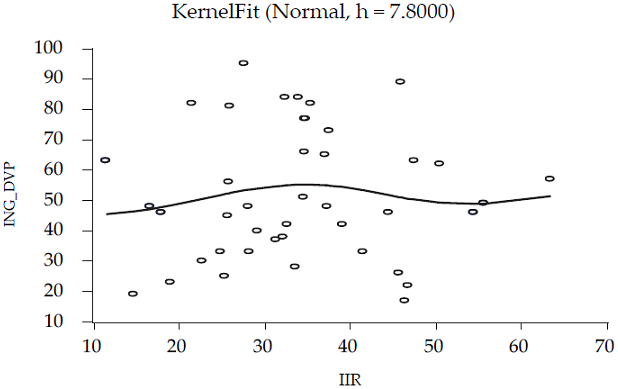
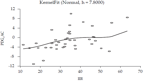
In order to make practical the debt intolerance measurement, Reinhart, Rogoff and Savastano (2003) focused on the indicator of sovereign debt called “Institutional Investor’s Country Credit Ratings” (henceforth IIR) prepared by the Institutional Investor.5 However, according to Figure 2, it is hard to pinpoint the relationship between the key indicator of external debt (PVD_GNI6) and IIR. The correlation coefficient7 between PVD_GNI and IIR is 0.017. But, the correlation between PVD_XGS and IIR is negative and relatively high (-0.23), which definitely does not make sense. That is, it is not expected that low debt indicator is associated with high probability of default on government debt obligation. Consequently, it indicates that it is not easy to define debtor’s club and external debt intolerance regions through only those two variables. Conversely, Figure 3 shows the other way the investors can analyze the country’s sovereign debt focusing on external vulnerability and it is reasonable to think about the positive relationship between high debt and strong external imbalances.
According to the debt intolerance approach, the inflation history is used to predict default. But, the inflation of the last eight years (from 1995 to 2002) is not associated with the IIR. At first glance, there is a very practical reason to believe that there is some relationship between inflation and sovereign risk. Certainly, countries suffering unrelieved inflation show frequently high interest rates and then they become more domestically indebted. Conversely, there is another reason to believe that this has been a phenomenon, at least since 1990s, with low likelihood to be related to increases in the external debt. Figure 4 shows the inflation across regions, and they were reduced to low levels even in developing countries where inflation is more difficult to be controlled.

But, why do countries without history of default attempt to avoid default for such a long period of time? The authors’ answer of the debt intolerance approach is associated with the interest that countries have in protecting their banking and financing system. It means that weak financial intermediation in many serial defaulters is associated with low penalty for defaulting. So, “The lower costs of financial intermediation disruption that these countries face may induce them to default at lower thresholds, further weakening their financial systems and perpetuating the cycle”(p. 13).8
Additionally, do debt-intolerant countries really borrow too much? According to those authors, at least from 1980s and 1990s, evidence shows that external borrowing was often driven by shortsighted governments that were willing to take significant risks to raise consumption temporarily, rather than to foster high-return investment projects. “The fact that the gains from borrowing come quickly, whereas the increased risks of default is borne only in the future, tilts shortsighted governments towards excessive debt”(p. 13).
Summing up, some countries borrow more than they should, and they borrow more because they are unable to find an alternative domestic source to support their imbalance. They also can live borrowing and defaulting as a way of life without focusing attention on protecting their weak banking and financial system. The external debt dynamics over time, specially indexed to foreign currency and international interest rates, is only the expression of the way they can borrow more; international investors lend more during exuberant financial cycles and earn higher returns than they would earn in developed economies.
Reinhart, Rogoff and Savastano (2003) are probably right when they emphasize the fact that default is a cyclical phenomenon and most likely serial defaulters are more prone to default during “sudden stops” in capital flows than the non-defaulters. The perception of the international investors is an important variable and can be expressed in ratings and credit risk measurements. It is also important that the history of inflation matters to build foreign investors’ perceptions.
But, what can be said about the role played by other factors such as the degree of dollarization and the maturity structure of the debt? Do these factors help to build the perception of foreign investors? That is, not only the degree of the external debt, but also its profile can be important to grade countries according to credit risk measurements. Is it fair to relate a country’s debt profile to domestic institutional weakness? In other words, why do some countries borrow the way they borrow?
Debt sustainability analysis
Now it is important to understand the situation that emerging market economies can experience when they are considered debt-intolerant countries and analyze the way they can deal with their debt in order to avoid default.
According to the standard debt sustainability analysis:
 [1]
[1]
where D(t) is the country’s external debt at time t, TB is its trade balance; r is the interest paid by the country on its external debt; g is the economic growth rate. In steady-state one can express the following relationship:
 [2]
[2]
where TB/Y is the steady-state ratio of the trade balance to output needed to stabilize the external debt ratio at D/Y.
To be closer to the recent movement of the external debt, three different changes in the expression [1] can be proposed. First of all, the current account instead of trade balance; second, as the majority of external debts in developing countries are US Dollars denominated, the debt denomination is incorporated in the model. Hence, not only the interest rate matters, but also the United States (US) dollar variability is taken into account in the expression; and, finally, the model weighs the participation of the US Dollar-denominated external debt. Then, the equation [1] can be expressed as:
 [1a]
[1a]
where e is the US exchange rate in terms of an international basket of currencies; W USD is the weight of the US Dollar-Denominated external debt in the total debt, and CA is the Current Account. Figure 5 shows the important role played by this component of the external debt when, in the early 1990s, the US Dollar-denominated debt averaged 40% of the total external debt in developing economies and in 2002 represented more than 60 per cent.

Source: World Bank (2004a).
Figure 5: Developing countries: currency composition of the long-term external debt, 1990-2002
After simple manipulation, the steady-state expression [2] can be written as follows:
 [2a]
[2a]
Taking into account the exogenous shocks, such as confidence, political and terms-of-trade shocks, ζ(t), [2a] can be expressed as a stochastic process as follows:9
 [2b]
[2b]
Figure 6 illustrates both situations for the “standard approach” of the external debt sustainability analysis and the other one added with the problem of foreign currency denomination of the external debt. According to expression [2] some countries can manage their external debt by implementing sustainable current account surplus (relative to Gross Domestic Product, GDP), as shown in the initial equilibrium A. But, once the interest rate is an endogenous variable (the higher the external debt, scaled to GDP or to exports, the higher the interest rate for future debt renegotiations),10 the model states that after the equilibrium A, the higher the debt-to-GDP (or debt-to-exports) is, the higher the interest rate for future payments will be.

The consequence is straightforward: the country must present very high current account surplus related to GDP. However, even if the country can increase its current account to GDP, it will not be insulated from more increases in its external debt, once most of its external debt can be foreign-currency denominated. In this context, there are many mechanisms to be revealed. First, if a country has elasticity to increase the current account,11 maybe because of either trade performance associated with depreciation in the domestic currency, or because the external income has increased faster than the domestic income. Second, and consequently, the international currency denominated external debt would have increased.
This especially dramatic dynamics of the external debt might take place only because the country’s initial level of debt (scaled by GDP or exports) may already have exceeded, or be close to exceeding the D/Y* level. Needless to say, non-anticipated external shocks in the foreign exchange rate and the international interest rate, besides the shocks in term-of-trade and domestic inflation, cause changes in the steady-state equilibrium, from CA/Y* to CA/Y*’, as shown in Figure 5. On the CA/Y*’ curve, with the same initial value of the external debt (D/Y*), the country must have a higher current account surplus, and, it is very likely to move on a steep curve and it therefore has to obtain a much higher current account surplus over time. However, some countries, mainly developing ones, seek more revenue from inelastic sources and they, therefore, borrow more abroad in foreign currency. During periods of exuberating capital flight they can probably finance their external imbalance, but when “sudden stop” takes place they default.
Finally, it is important to consider the rapid growth of the domestic government debt in the 1990s. It is fair to say, according to the experience in Brazil, Argentina and Turkey, that the domestic government debts are denominated either in foreign currencies or in some short-term interest rates. “These trends suggest that domestic debt intolerance can manifest itself in a manner similar to external debt intolerance” (Reinhart, Rogoff and Savastano, 2003, p. 50).
Discussing the effects of debt intolerance for debt sustainability analysis, it is necessary to recognize that the interest rate paid on debt is an endogenous variable, which depends on the debt-to-output (or debt-to-exports) ratio. The interest rate on debt to private creditors can increase with the debt level. Additionally, sustainability analyses need to take into account that the initial level of debt may already have exceeded.
According to this standard debt sustainability model, emerging market economies can experience difficulties in overcoming external imbalances and therefore they default. However, they default not exactly because of their history of default and inflation. They default because of the way they borrow. In a prospective analysis even if they borrow less they can default; even if they present commitment to keep inflation at low levels, they can default; and, finally, even if they defend low exchange rate volatility,12 default can be their destiny.
Econometric findings: a panel model
The panel approach allows for two basic models: fixed and random effect models, both of which admit static and dynamic specifications. The fixed effect model, also known as Least Square Dummy Variable (LSDV), is a generalization of an intercept-slope-constant model for panel analysis, introducing a dummy variable to capture the effects of omitted variables that are constant over time.
In this specification, the individual-effects can be freely correlated with the regressors. Their estimation is, in fact, the own estimation of the model of multiple regressions with binary variables for each one of the n units of the analysis, in such a way that their introduction will cause the intercept of the regression to be different for each one of these variables and pick up the heterogeneity among them. The ordinary least square (OLS) estimator known as LSDV will be consistent and efficient. On the other hand, the random-effect model specification considers the individual-specific effects as random variables, assuming no correlation between the individual effects and the other random variables, where the estimation was pursued by using the Generalized Least Square (GLS).
As first step, the econometric procedures take the following general expression:
 [3]
[3]
where:
Table 2 shows the first empirical results by within transformation, or alternatively called as fixed effects model. The important thing about equation [3] is that the unobserved effect α i has disappeared. It means that equation [3] was estimated by OLS using the time variation in y and x within each cross-sectional observation. Hence, the unobserved α i is a parameter to be estimated for each country i, that is, to be estimated along with the β i .21 We run several variants of equation [3].
Table 2: Empirical results, 1990-20021. Fixed effect model

Notes: 1/ Even though we ran other equations using different methods, only the best results in terms of t-test and/or expected signal are shown. 2/ All estimations were run by using robust standard error. T-test statistics in parentheses. 3/ We reported only Monetary and Financial System, instead of reporting Monetary System and/or Financial System because it was our better result. 4/ Unbalanced panel with 57 individuals, longest time series with 13 and shortest time series with 8 (1990-2002). 5/ Wald (joint) X 2(2). 6/ AR(1) test N(0,1).
First of all, there is strong cross-country evidence, for the period 1990-2002, that high GDP is positively correlated with high external debt; second, even statistically non significant, high growth rates in external debt are related with lowers growth rates in GDP; third, there is no evidence proving any sort of reasonable relation between growth of the external debt and either inflation or the size of the monetary and financial system.22
It is very important to highlight that the same equations were run using different measurements that express the same reasonable idea of monetary policy credibility: the inflation measured by CPI and the variance of inflation measured by five-year moving average and only the best results in terms of t-test statistics and/or coefficient signal were reported. We also preceded exclusion and restrictions tests to evaluate a restrict model against an irrestrict one, according to F-statistic. Variance of inflation was tested because some countries can mantain the high interest rate longer with the intention to build credibility because they recently had undergone hyper-inflation episodes.
Fourth, high current account deficit to GDP ratio is statistically related to changes in the external debt, which suggests that there is some evidence in favor of the external vulnerability as an important sign of highly indebted countries. Taking the debt to GDP ratio, were ran other set of equations. Once more, inflation (or variance of inflation) and the size of the monetary system were not statistically significant at all, what means that countries that have experienced high inflation are not the same as those with high external debt; additionally, the size of the monetary system is not statistically significant, even the negative sign can convey the idea that the country with large monetary system is less indebted.
It was tested if severely indebted countries have experienced pegged exchange regimes and there is no empirical evidence in favor of this idea. It means that the choice of the pegged exchange rate regimes and the subsequent collapse in the developing economies did not help to predict the external debt dynamics, even though it can be narrowly associated with domestic federal debt and default of this debt. Finally, considering the variables that can express the debt profile (maturity structure, interest rate and currency-denomination), it is absolutely fair to say that all those explanatory variables are statistically significant to explain the external debt dynamics during the 1990s in developing countries.
Of course, the within transformation could not be the best estimator, especially when the unobserved effect is uncorrelated with all the dependent variables. In this case, random effect estimators might be more attractive. Then, it is important to know which is the most appropriate model. According to Frees (2003), it depends on the available information and the estimation goals. If, for example, the main concern of the analysis will be to test the effect of the variables where the individuals are classified in groups, then the random effect specification is more appropriate. In Hsiao (1999, p. 42): “The fixed-effects model is viewed as one in which investigators make inferences conditional on the effects that are in the sample. The random-effects model is considered as the one in which one can make unconditional or marginal inferences with respect to the population of all effect.” One way to decide whether to use a fixed effects or random effects model is to test for misspecification according to ratio F or, alternatively, the Hausman Test (see Hsiao, 1999, p. 48).
Thus, the set of equations already reported in Table 2 was run according to a random-effect model23 and the relevant results remained almost the same (see Table 3), except in instance:24 the size and development of the monetary and financial system became statistically significant and with positive signals and these results contradict the debt intolerance approach because it believes in a certain indisposition of the developing countries’ governments to protect their monetary and financial system. That is, the most indebted developing countries are the same with the largest domestic credit provided by banks and the largest market capitalization.
Table 3: Empirical results, 1990-20021. Random effect model

Notes: 1/ Even though we ran other equations using different methods, only the best results in terms of t-test and/or expected signal are shown. 2/ All estimations were run by using robust standard error. T-test statistics in parentheses. 3/ We reported only Monetary and Financial System, instead of reporting Monetary System and/or Financial System because it was our better result. 4/ Unbalanced panel with 57 individuals, longest time series with 13 and shortest time series with 8 (1990-2002). 5/ Wald (joint) X 2(2). 6/ AR(1) test N(0,1).
Consequently, it is fair to remark that:25
If the debt intolerance approach were right, it would be able to see some significant and negative estimated parameters for the inflation, variance of inflation, domestic credit (or scaled by GDP), market capitalization (or scaled by GDP), or interactions of these variables such as the Monetary and Financial System. We know that debt intolerance cannot be reduced to this analysis, but it supports the ideas that debt intolerant countries operate under weak monetary and financial system and under inflation, and that their governments have no concerns about probability to default.
It was not reported any evidence regarding tax systems and most importantly, the debt intolerance approach can be correct about the fact that countries where tax system avoidance is high tend to have greater difficulty to pay the debt. However, if the profile of the external debt is so important, according to the empirical findings, even if the government faces relatively elastic tax sources to honor debt payments, it would not be enough once the developing countries’ debts face high foreign currency volatility and higher international interest rate to pay debts than their domestic interest rate.
So, even with intense effort from domestic authorities of the developing countries in order to improve output growth, building credible monetary policy and/or strengthening the tax system, the external debt dynamics associated with foreign-currency denomination and also concentrated in small number of currencies in short-tem maturity structures may cause default.
Even if we have not directly tested the main original sin hypothesis, that explains why some countries cannot borrow abroad in domestic currency, even domestically for the short term we presented a lot of empirical inquiries concerned with the way developing countries borrow abroad and how important this is for the debt dynamics. It seems that some countries default because of the way they borrow and according to the original sin arguments the way they borrow is strongly associated with the global imbalance and causes, therefore, currency mismatches. In other words, the original sin hypothesis can be considered the alternative to the null hypothesis (debt intolerance).
Finally, Reinhart, Rogoff and Savastano (2003) are apparently right when they argue that there are some critical shortcomings in the standard sustainability exercises and the recognition of other factor, such as the degree of dollarization, short-term interest rates and the maturity structure of a country’s debt are actually different manifestations of the same underlying institutional weaknesses. However, these authors are concerned only about the domestic institutions and differently this article believes that international institutions matter as well.
Final remarks
The empirical evidence presented in this work is comprehensive and straightforward in order to show reservations about the hypothesis supported by Reinhart, Rogoff and Savastano (2003). The inflation (or variance of inflation) and the size of the monetary-financial system barely explain the sovereign debt dynamics since 1990. There is no evidence in favor of the idea that debt intolerant countries are not concerned about their financial system and they are not the same living with high inflation rates, even though developing countries show higher inflation rates than developed ones.
The external debt dynamics preserve the traditional foundations associated with the maturity structure (predominantly short-term debts), interest rates paid to the obligations (most of them are higher than the domestic interest rates) and, last but not least, the foreign-currency denominated debt. As we know the US dollar-denominated debt can reach 80% of the total debt. From this last feature derives the idea that the external debt can not be manageable only by domestic governments. That means directly that even under extraordinary economic growth rates and credible monetary and fiscal policies, developing economies can not avoid US dollar volatility. More than symptoms of the history of default and inflation, the way the developing economies borrow abroad is remarkable. They definitely suffer from the “original sin” since they have inability to borrow abroad in their own currencies.