Introduction

The case of Mexico offers an interesting example in the analysis of the evolution of regional disparities in developing countries that have changed their policies from those of a state-led economy to those of economic liberalization and trade openness in the 1980s. The recurrent economic crises and the transition to economic reform and liberalization have aroused much interest as the gap in per capita GDP (Gross Domestic Product) among regions has risen since the mid-1980s. This problem, moreover, is shared with other developing countries that have undergone transformation in economic policies, for example, China (^{Demurger, 2001}; ^{Fujita and Hu, 2001}; ^{Yao and Zhang, 2001}). In spite of this, Mexico still suffers from a lack of a well-defined and coordinated regional policy as such. Regional policy has been limited to the spatial impact of national policies, which have tended to increase concentration of industry and population in some areas (^{OECD, 1997}).

A number of studies have analyzed the determinants of regional growth in Mexico, focusing on different aspects and using different methodologies (^{Cermeño, 2001}; ^{Chiquiar, 2005}; ^{Costa-Font and Rodríguez-Oreggia, 2005a} and ^2005b; ^{Esquivel, 2000}; ^{Esquivel and Messmacher, 2002}; ^{García-Verdú, 2002}; ^{Messmacher, 2000}; ^{Rodríguez-Oreggia, 2002}). In all cases, the findings show that there is increasing polarization between the Mexican states, richer states becoming richer and experiencing higher growth. One aspect that has not yet been analyzed in detail is the dynamics of the regions in terms of income and growth. ^{García-Verdú (2002)} analyzed the mobility between different levels of income, finding that mobility is low. However, there is a gap in the analysis of the interaction between income and growth and the factors determining such mobility.

The purpose of this paper is to focus on aspects derived from convergence and divergence, determining the dynamics and their determinants among regions in Mexico. In doing so, we shall determine the standard β and σ convergence. Moreover, we go further in the analysis of regional disparities in Mexico and then go on to calculate the transition probabilities between four different categories based on growth and income (winners, falling behind, catching up and losers). We apply a probabilistic model to those categories in order to determine which factors affect such mobility between categories.

Speed of convergence

The work of ^{Barro and Sala-i-Martin (1991}; ¹⁹⁹²; ¹⁹⁹⁵⁾ on the neoclassical convergence of per capita GDP among countries and regions initiated a stream of works investigating the speed at which economies tend to close or increase disparities. Although criticized (^{Quah, 1993a}; ^1993b; ¹⁹⁹⁶), this approach to the evolution of disparities has developed two main measures of long-term growth analysis through the beta and sigma coefficients. To some extent the process of convergence is associated, in general, with recession periods while the divergence is found in periods of economic boom (^{Chatterji and Dewhurst, 1996}). From this, some regions are seen to be winning, while other regions are losing.

Following the work of ^{Barro and Sala-i-Martin (1991}, ¹⁹⁹², ¹⁹⁹⁵⁾ on the patterns of growth at regional levels there have been streams of works interested in investigating the common speed at which economies converge to their own steady state. These ideas were first proposed by ^{Abramovitz (1986)} and operationalized by ^{Baumol (1986)}, and are supported by the neoclassical growth theory under the common assumption of diminishing returns to capital.

The implication behind the latter assumption on neoclassical models is that each addition to capital will generate a more than proportional addition in output when capital is small, and small addition when capital is large. Consequently, if the only difference across economies is the initial capital stock, poor regions (with small capital stock) will grow faster than rich regions (with large capital stock), leading to convergence.

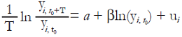
The literature uses the β coefficient to measure the speed of convergence. There is β convergence if, on average, initially poor regions are growing faster than rich regions. The speed of convergence, or beta coefficient, is estimated through the following equation (^{Barro and Sala-i-Martin, 1991}; ¹⁹⁹²; ¹⁹⁹⁵⁾:

[1]

Where the left side is the average annual rate of growth of per capita GDP and the right side the initial level of per capita GDP of a set of regions between time t₀ and t₀+T. The β coefficient is the absolute β convergence coefficient, without conditioning on any other characteristic of states. The model can be modified to include some variables, to control for differences in other characteristics and to calculate conditional beta convergence.

The results are presented in Table 1 using Ordinary Least Squares. It presents regressions for specific time periods, the period 1970-2001 is the whole sample, which is then broken down into two main sub-periods comprising the period before trade liberalization and economic reform, 1970-1985, and the period after these changes, 1985-2001. These two periods will constitute the axis on which the analysis in this paper will be based, as this breakpoint constitutes a structural change in the economy¹ (for example, ^{Lächler and Aschauer, 1998}, using national data found a significant test for structural change in 1985-1986). These periods have been used in order to obtain better results in the analysis as demonstrated in ^{Rodríguez-Oreggia (2002} and ²⁰⁰⁵⁾ and ^{Chiquiar (2005)}. In addition this period covers Mexico’s inclusion in the North American Free Trade Agreement (1994-2001) [NAFTA].

Table 1: Absolute beta convergence 

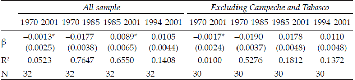
* Not statistically significant at 10%. All sample calculations include a dummy control for Campeche and Tabasco.

We also present the results both with and without the oil states, Campeche and Tabasco, as these experienced very high rates of growth at the end of the 1970s and beginning of the 1980s as a consequence of the oil boom.²

Using either the whole sample or with the exclusions, the overall period 1970-2001 does not show evidence of convergence as the coefficient is not significant.

Dispersion across states

Another important guide to the evolution of regional disparities is how dispersed is the per capita GDP. Dispersion across states is typically measured by the standard deviation of the natural logarithm of the states’ real per capita GDP. This concept is called in the literature sigma and it measures how the distribution of income evolves over time (^{Sala-i-Martin, 1996}), with sigma convergence existing when the coefficient gets smaller. The existence of sigma convergence may imply the existence of beta convergence, but this does not necessarily work the other way around (see for example ^{Sala-i-Martin, 1996}).

To assess the extent to which there has been a σ convergence process across states in Mexico we calculated the standard deviation of the natural logarithm of the real per capita GDP since 1970 as depicted Figure 1. These findings adjust to the beta coefficients, the sigma coefficient decreasing in the period that the beta suggests convergence, while in the period that sigma increases the beta suggests divergence.

Note: The Exc category excludes Campeche and Tabasco.

Figure 1: Sigma convergence 

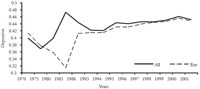
Results are consistent with the findings of ^{Juan-Ramon and Rivera-Batiz (1996)}, who found convergence in the period before 1985 and divergence thereafter. ^{Cermeño (2001)} also found a decreasing per capita GDP rate during the period 1970-1995. ^{Chiquiar (2005)} and ^{Rodríguez-Oreggia (2002)} also confirm those findings. In all cases it is apparent that it will become more difficult to close differences between rich and poor states, as disparities among factors inciding in convergence is also high. For example:

^{Rodríguez-Oreggia and Rodríguez-Pose (2004)} have found that the main reason behind the convergence process before 1985 was the rate of growth of public investment and not the infrastructure created with it, offsetting even the possible impact from human capital; while the reduction in public investment after that period is not significant for regional growth.

If we want to compare with Europe, ^{Boldrin and Canova (2001)} show that a process of convergence occurred there in the period 1950-1973 while in subsequent periods the process stops. They argue that the period of convergence corresponds with an absence of regional policies and with the increase of trade, while after the implementation of regional policies the increase in trade was not accompanied by any reduction in disparities. In the USA the process of convergence experienced throughout the century has halted since 1979, although the reasons are said to be still unclear (^{Bernat, 2001}).

These results are also similar to findings in other developing countries under conditions of economic liberalization and with few areas with strong geographical advantages: for example, in China, where differences between coastal and interior areas increased during the 1980s and especially during the 1990s due to globalization and further economic liberalization, the coastal regions, with the geographical advantage of access to the sea, show a convergence process (^{Demurger, 2001}; ^{Fujita and Hu, 2001}; ^{Yao and Zhang, 2001}).

Dynamics of regional income and growth

However, the traditional work on convergence based on neoclassical assumptions has been, criticized. ^{Quah (1993a}; ^1993b; ¹⁹⁹⁶⁾ suggested that the standard neoclassical models assume exogenous processes, where little could be said. In addition, the neoclassical work tends to cluster around a rate of two per cent, derived from a problem called the Galton’s fallacy when running growth against the mean. Quah, then, proposed the use of Markov chains in order to analyze the dynamics of transition for different levels of income. ^{García-Verdú (2002)} used this technique to analyze the income dynamics of the Mexican regions, showing low mobility between income groups, although this study offered no further analyses of the factors determining such mobility.

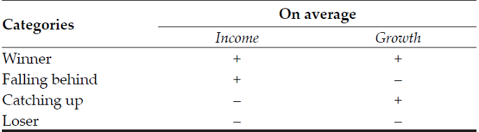
In these sections we will follow the Markov chains methodology, although with a different approach and we shall take it a bit further. We have clustered regions not only according to income but also to growth. In so doing, we have applied four levels or categories. Regions with higher than average growth and higher than average initial per capita GDP can be classified as winners. Regions with less than average initial per capita GDP but higher than average rates of growth are classified as catching-up areas. Regions with less than the average in both variables are losers. Finally, regions with higher than average initial per capita GDP, but lower than average rates of growth can be described as falling-behind regions. To aid understanding, Table 2 displays the categories.

Table 2: Categories of regions 

The Markov chains and transitional probabilities allow one to see the mobility between levels and the methodology can be found in ^{Quah (1993b)} and ^{Ljungqvist and Sargent (2000)}. A Markov Chain is a sequence of events for which the probabilities of outcomes or states depend on a previous action. A transition probability matrix shows the probability of moving from one initial state (rows) to any other state (columns).

We have calculated the transition probabilities for the Mexican regions, presented in the following matrices, for all the states and also excluding the oil regions. Each cell shows the probability that a state starting at one of the levels in the rows, will end at a given level in the column. For example, the 44 in the first matrix indicates that a state being a winner in the first period has a 44 per cent probability of remaining in the same winning position at the end of the period, while the 56 per cent indicates that such a probability is attached to a winning region in the first period moving to a falling-behind condition in the latter period.

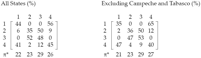
Categories: 1= Winner, 2=Catching Up, 3= Loser, 4=Falling Behind.

Transition probabilities, 1970-2001 

Mobility is low, as can be noted from the high values in the diagonal lines in the matrices. One important point to note is that regions at levels above the average at the beginning tend to remain at such levels, either as winners or falling behind, but they do not move to levels lower than average in income such as losers or catching-up. Regions starting as losers tend to remain at the same level or move to a position of catching-up, but they do not move to higher than average income categories. This means that poor regions tend to remain poor. In addition, regions starting as catching up have a greater probability of moving to a falling behind position (nine or 12 per cent) than to a winner position (six or two per cent). The ergodic distribution (π*) shows that the concentration of regions is approximately equal across the four categories.

In order to depict the evolution of such dynamics we have mapped the categories of the states for two periods. Map 1 presents the distribution of categories in the period 1970-1985.

Map 1: Distribution of income and growth, 1970-1985 

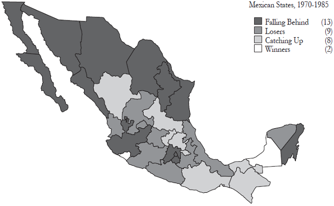
We can note from the map that the northern states, Mexico City and surrounding states fall within the falling behind category, while southern states are in the catching up category. The reason behind poor states were catching up can be found mainly in the growth of public investment mainly in the decade of the seventies and beginning of eighties (^{Rodríguez-Oreggia, 2002}). However, the picture changes drastically when looking at Map 2 for the period after 1985.

Map 2: Distribution of income and growth, 1985-2001 

Map 2 shows the distribution of categories for the period 1985-2001. In this period characterized by trade liberalization and reform, the northern states fall within the winner category, as do Mexico City, Jalisco and Aguascalientes. The southern states now fall within the loser category. This may be happening for several reasons: the fall in public investment from central government (^{Rodríguez-Oreggia and Rodríguez-Pose, 2004}); concentration of public investment in richer regions (^{Costa-Font and Rodríguez-Oreggia, 2005a}; ^{Messmacher, 2000}), and the geographical advantage for trade for some regions (^{Costa-Font and Rodríguez-Oreggia, 2005b}).

Up to this point we have analyzed the mobility between categories, the results of which are in harmony with the findings of ^{García-Verdú (2002)} using only per capita GDP groups without considering growth. However, an interesting question that has been overlooked in previous works is: what factors determine such mobility? The next section will address this issue.

Factors and dynamics

In order to identify the factors that will contribute to regions moving from one category to another, we shall apply a multinomial logit. We briefly summarize the model to conserve space, but a full description can be found in ^{Greene (2003)}. Assuming that each region falls within a category every period, according to a set of factors, the probability that a region i falls in a category j depends on a vector of i’s variables (Z _i ):

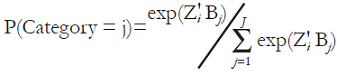[2]

P follows a logistic conditional probability function and β _j represents a Kx1 vector of coefficients for category j. These parameters are estimated using maximum likelihood estimations (^{Greene, 2003}) and they must be read against a base category. The data are from the INEGI database (^{INEGI, 2003}) [Instituto de Estadística, Geografía e Informática), which was published at five-year intervals from 1970 to 1985, then in 1988, and then annually from 1993 to 2001. We have used time spans of five years in order to construct panel data³ and calculated the position of each region in the four different categories used in the previous section.

As we have used four categories, one has to be taken as the base, so here we take the losers position and the coefficients of the other three categories should be read as the probability of that category against the base category.⁴ As explanatory variables we include the initial average years of schooling of the population aged 15 and over (School) taken from the Statistical Annexes to the Presidential Address to the Nation (various years), the initial stock of public capital per capita (Public K) from ^{Rodríguez-Oreggia (2002)}, a dummy for the populist years (1970-1982), a dummy for the NAFTA years (1994 onwards), a time trend, a dummy for Campeche and Tabasco (Oil) and a dummy for Center states.⁵

Results are presented in Table 3 for the different periods, including the sample as a whole as well as that excluding the oil states. The category base is Losers, thus all coefficients should be interpreted compared to that base, i.e. the probability of being in a determined category compared to that same factor in the base category.

Table 3: Multinomial logit. Dynamic of regions between four groups 

Note: * NO-significant at 10%

The coefficients for schooling are highly relevant for mobility, particularly with higher coefficients for the period after 1985 for richer regions, while in the period starting in 1970 the significance is blurred. Why this may happen? A plausible explanation is that skills may work better under a reformed and less regulated environment and then have an impact on growth. According to ^{López, Thomas and Wang (2000)} the policy environment in a country could determine what people do with their education and skills. In a country with reformed policies aimed to improve trade and investment and with reduced distorted prices, returns to education can increase and enhance the impact of education on growth. If we take this as explanation we can find that in the period before 1985 the Mexican economy was highly regulated and protected. After the entrance to General Agreement on Tariffs and Trade (GATT), the country has been one of the more opened to trade in the world, fitting to the suggestion of López et al.

The coefficient for school is still much higher for richer and growing states. This is because of the still higher disparities in terms of education among regions. Although the country in general has experienced remarkable progress in education attainment alongside with income disparities (^{De la Torre, 1997}), the relative position of states regarding such issue may still remain equal (^{PNUD, 2005}).

The coefficients for public capital are highly significant for Winners and Falling Behind categories. There is plenty of evidence of the allocation of public investment for infrastructure benefiting more the richer states (^{Costa-Font and Rodríguez-Oreggia, 2005a}), thus the evidence from Table 3 suggests that public capital measured as the stock of public infrastructure creates a dynamics where there are advantages for richer regions, while the effects of low income states is lower or blurred. These findings reinforce the idea of a core-periphery pattern (^{Krugman, 1991}) for the Mexican regions, as the economic activity has concentrated in the border states, and Mexico City still has an important share of the production. This leads to an increase of disparities among regions, especially if carried out in order to increase interregional transport communication (^{Martin and Rogers, 1995}), which has been the case in Mexico, as the intraregional communication infrastructure has been left aside historically (^{Chias, 1995}).

The period of populism is significant in the models for winners and catching up but not for the falling behind category. This period was characterized by a high level of government spending made without any underlying economic logic (^{Bazdresch and Levy, 1991}). Other studies have found that the growth of such spending clearly affected the rates of growth of the Mexican regions leading to a faster growth for poor regions, but not affecting greatly the quality of the infrastructure (^{Rodríguez-Oreggia, 2002}). Then, the inclusion of this variable partially reflects such effect.

The NAFTA period is important only for the winner category when including the whole sample and in the period 1970-2001. But the same variable is not significant for the period 1985-2001. This would suggest that categories were not effectively influenced by the NAFTA in the liberalization period, the regions for the most part remaining in the same categories since the 1985 structural change. This may be explained in terms of the different levels of specialization of industry in the states, which have displayed a very different pattern over the last few years (^{Messmacher, 2000}). Also, it is likely that the trade openness in the middle of the eighties has had a more important effect on the whole economy than that derived from NAFTA.

Conclusions and discussion

This paper has made further contributions to the analysis of regional inequalities in Mexico. We have used a dataset from 1970 to 2001 and both cross-section and panel data analysis. We examine regional disparities using the standard β and σ convergence analysis and the Markov chains and transition probabilities according to four groups following income and growth (winners, falling behind, catching up and losers) and factors affecting the dynamics of those groups.

Results from the analysis show that the dynamics of disparities among the Mexican states has been propelled especially from differences in the endowments of human capital and public infrastructure, fostering a deepening of a core-periphery pattern rather than increasing the possibilities of the poorest states to catch-up with richer states. The results from this analysis show that public investment fosters the reinforcement of the categories selected, especially for Winners and Falling-behinds which have higher income, i.e. it fosters convergence clubs, in those areas which are also taking most of the benefits from the trade openness. Differences in human capital endowments also foster convergence clubs according to our evidence. Although human capital has taken effect on growth especially after the trade and liberalization period, differences among regions still prevail. However, we only considered a stock of education but not quality, which also could make a difference on the impact on growth. Moreover, it should be noted that poorer states in Mexico have an unequal access to education, especially after secondary levels (^{Salinas and López-Acevedo, 2000}).

The lack of regional policies for Mexico becomes evident. In the European Union, where regional policy is one of the strongest focus of investment, it has been one of the main instrument for redistribution (^{Boldrin and Canova, 2001}). In Mexico, public investment has not been effectively used as an instrument for redistribution or as an engine for regional growth, but more as a pork-barrel devise seeking electoral pay-off (^{Costa-Font, Rodríguez-Oreggia and Luna, 2003}).

In the case of public infrastructure, although the several National Development Plans have set as one of the aims to improve the economic capacity of the states through an increase in the direct implementation of public works of local interest, there is ample evidence of the regressive allocation of such investment. Those Plans also have set as aim to reduce inequalities among regions, and also allocate resources to foster medium-size cities, etc., leading to a lack of a clear-cut objective.

If public policies want to influence the pattern of regional development and reduce disparities and desincentivate the creation of convergence clubs, they first have to set a clear- cut aim for a coordinated regional policy. According to ^{De la Fuente and Vives (1995)}, a regional policy should follow one of three possible criteria: first, need, counterbalancing the disadvantages of poor regions through public investment and increasing human capital, allocating more resources to poor regions but meeting the additional needs from increasing population in richer ones; second, efficiency, aiming to maximize national income, allocating then resources to regions with higher returns to investment, but redistributing ex-post through taxation; or third, a neutral criterion ensuring not to give excessive advantage to any region. Here, the role of the Mexican government is to determine what kind of regional policy should address and to consider, given the evidence presented in this paper on the creation of rich clubs of states whether it is socially, morally or politically unacceptable for different parts of the country to experience large differences in standards of living, and also to consider whether such regional disparities may reduce future possibilities for national growth and larger trade integration with North American countries.