nova página do texto(beta)
 Inglês (pdf)
 Artigo em XML
 Referências do artigo
 Enviar este artigo por email
 Citado por SciELO
  Similares em
SciELO
Similares em
SciELO 
 Permalink
1. Introduction
The current understanding of the structure and evolution of massive stars is based on extensive theoretical models (Brott et al. 2011; Ekström et al. 2012; Heger et al. 2000; Maeder & Meynet 2000; Paxton et al. 2019), which, however, have many tunable parameters (e.g., mass loss rate, mixing length, among others). Constraints on these calculations and additional insights into the stellar structure are gleaned from theoretical atmosphere models from which synthetic spectra are produced and can then be compared with observations (Hillier & Miller 1998; Hillier & Lanz 2001; Puls et al. 2005; Hubeny & Lanz 1995). Through this comparison, fundamental stellar parameters are derived.
An underlying assumption in nearly all theoretical models is that the observed spectrum arises in a spherically symmetric atmosphere and wind. Thus, the spectra of binary systems are generally modeled as the sum of the individual spectra arising in each of the two stars. However, massive stars emit intense ultraviolet radiation that drives a fast and dense stellar wind. If a binary system is composed of two massive stars, their mutual irradiation and wind interactions produce localized emission and absorption. Because an observer’s line of sight to these localized line-emitting regions changes over the orbital cycle, their contribution to the observed spectrum produces orbital phase-dependent variations in the shape of spectral lines. This is referred to as line profile variability which, if significant, introduces uncertainties in the fundamental stellar parameters as derived from fitting spectra of single stars. Particularly noteworthy are the challenges involved in determining the contribution to the spectrum from a wind collision zone (WCZ).
The first observational evidence pointing to the presence of a WCZ in WN binary systems was obtained for V444 Cyg, HD 211853 and HD 90657 by Koenigsberger & Auer (1985). These authors detected orbital phase-dependent variations in the shape of the C IV λ1540 P Cygni, consistent with a WCZ dominated by the WR component of the system. Shore & Brown (1988) used higher spectral resolution UV data of V444 Cyg to reach a similar conclusion. Auer & Koenigsberger (1994) modeled the line profile variability in the N IV λ1718 line in V444 Cyg assuming it was due to wind eclipses, and found discrepancies between the model and the observations attributable to a WCZ. A similar analysis of the P V λ 1117 line observed in the FUV spectrum of HD 5980 led to the conclusion that the WR wind velocity structure is truncated on the hemisphere facing the companion due to the WCZ (Koenigsberger et al. 2006). These studies did not attempt to model the actual emission arising in the WCZ, an issue partially addressed by Luehrs (1997), who assumed that emission line sub-peaks in C III λ5696 observed in the WC7+O5-8 binary HD 152270 could be modeled as two separate emission lines originating in the outflowing WCZ streams. The same geometrical model has been applied to several other binary systems (Hill et al. 2000; Hill 2020; Hill et al. 2018) leading to the conclusion that the excess emission produced in the WCZ is responsible for between 10%-100% of the observed line emission, depending on the spectral line and the binary system. A somewhat different approach was employed by Flores et al. (2001) who analyzed the excess emission over that expected from an unperturbed, spherical wind in the V444 Cyg binary, concluding that the WCZ contributed no more than 12% of the total He II λ4686 line emission. The major deficiency in the simple models is that they rely on the assumption that superposed peaks on a line profile can be attributed uniquely to excess emission. This neglects the possible presence of superposed absorption that can cut into the broad underlying emission, resulting in an appearance that mimics the presence of emission peaks. In addition, in many cases there is no certainty that the underlying stellar wind line profile can be approximated with a stellar wind model line profile unless this profile is computed self-consistently with the perturbations introduced by the collision process.
The collision of two supersonic winds produces a double shock structure between them where radiation is emitted in wavelengths ranging from X-rays to the radio spectral regions (Corcoran 2003; Nazé & Rauw 2017; Pittard 2009; Pittard & Dawson 2018; Russell et al. 2016; Richardson et al. 2017; Lamberts et al. 2012). The shape of the collision region is determined primarily by the mass-loss rates and the wind velocities, and in its simplest representation, the shock region can be thought of as conical, and folded towards the star having the weaker wind momentum (Prilutskii & Usov 1976; Cantó et al. 1996). In reality, however, the geometry and physical conditions within the WCZ are significantly more complex, and require 3D numerical simulations to be understood. Complicating factors include the Coriolis effect which breaks the symmetry of the shock cone with respect to the line connecting the two stars, the UV radiation field from the stellar continua and from the WCZ itself which can alter the pre-shock wind structure, and the cooling efficiency of the shocked gas which determines the thickness and radiating properties of the shocked region. Simulations taking these factors into account show that binary systems having different combinations of wind, stellar and orbital parameters can result in a WCZ that is either a dominant contributor or a relatively minor perturbation (Pittard 2009; Russell et al. 2016; Richardson et al. 2017; Pittard & Dawson 2018). Thus, in a sample of massive binary systems, each binary may have a unique set of parameters, and these result in a WCZ whose emitting properties differ from those of any other binary. This makes it challenging to determine general properties that characterize the impact of a WCZ on the observed spectrum. It is equally challenging to ascertain the relevance of the WCZ on the emission line profiles and their variability.
The close binary system in HD 5980 provides what could be described as nearly laboratory conditions for studying wind-wind collision physics. Specifically, it is a system in which the masses and orbital elements have remained constant during the more than 60 years over which it has been observed but in which one of the components has suffered significant luminosity and wind structure changes. HD 5980 is located in the periphery of the young stellar cluster NGC 346 in the Small Magellanic Cloud, and consists of two binary systems. The first of these displays a nitrogen sequence Wolf-Rayet (WN) type spectrum, indicative of chemical abundances corresponding to an advanced evolutionary state (Koenigsberger et al. 2014; Shenar et al. 2016; Hillier et al. 2019). Its two stars are massive (≈ 60 M⊙), luminous (≈ 106 L⊙), and in a relatively close and eccentric orbit (P =19.3 d, e = 0.3). They are named Star A and Star B. The second binary system displays a late Of-type supergiant spectrum and is in a highly eccentric 97 d orbit with an unseen companion. This system, named Star C, contributed in 1978 approximately 40% of the light to the HD 5980 system (Perrier et al. 2009). There is at present no evidence indicating that both binary systems are gravitationally bound to each other. Hence, we focus hereafter on the Star A + Star B system.
Prior to its confirmation as a binary system, Smith (1968) and Walborn (1977) classified the observed WR spectrum as WN3, with the latter author remarking on the absence of N IV λ4058 in spectra of 1973 and 1977. Curiously, about a decade later Niemela (1988) detected this line, prompting her to propose WN3 and WN4 for Star A and Star B, respectively. Unknown at the time was that the system had initiated in ≈ 1980 a slow brightness increase and that all the WR emission lines, including λ4058, were becoming stronger. In 1993-1994, HD 5980 suffered two sudden and strong eruptive events, expelling ≈ 10−3 M⊙ (Barbá et al. 1995; 1995ApJ...452L.107K). The absence of λ4058 in 1973 and 1977, its presence after that, and the appearance and strengthening of numerous UV Fe V and Fe VI lines leading up to the eruptions prompted Koenigsberger et al. (1995) to propose that the erupting component was the object responsible for the WR-type spectrum. At that time, however, it was believed that the dominant spectrum arose in Star B. However, subsequent RV measurements of these same Fe V/IV features showed them to instead follow the orbital motion of Star A, and Barbá et al. (1995) found indications of a large hydrogen abundance in the post-eruption spectra, not expected to be present in a bona fide WNE type star, as Star B was believed to be. Hence, the eruptive events were associated with an LBV-like process originating in Star A which, at the time, was believed to be an Of-type supergiant.
At the peak of the eruption, the dominant spectral type was WN11, as determined from spectra in the optical range (Heydari-Malayeri et al. 1997) or B1.5Ia+ from UV spectra (Koenigsberger et al. 1996). After that, the brightness declined rapidly until ≈ 1996, remaining at an apparent plateau until ≈ 2002, after which it declined gradually. Currently, the N IV λ4058 emission is still significantly stronger than N V λλ4603-21, indicating a WN6 spectral type. All strong lines follow the orbital motion of Star A.
Moffat et al. (1998) reviewed the behavior of HD 5980 prior to, during, and following the eruption and concluded that Star A must have been an O-type supergiant that through the eruptive process had transitioned to a WN star. They also proposed that the spectrum of this assumed O-type star and of Star B had been drowned out by wind collision emission, and proposed that the WCZ spectrum imitated that of a WN star. Applying the Luehrs method to spectra obtained in 1991/1992, they concluded that the WCZ extended perpendicular to the semimajor orbital axis and that the emission-line RVs could not be interpreted as representing in any way the orbital motion. This conclusion is in stark contrast with the cmfgen radiative transfer model fit obtained to HD 5980’s λλ1200 -10000 spectral energy distribution and emission line intensities observed in 1999 and in 2014 (Koenigsberger et al. 2014; Shenar et al. 2016; Hillier et al. 2019). Thus, the bulk of the emission must arise in the stellar winds which, however, does not exclude the presence of additional emission and absorption arising in the WCZ.
The current scenario for HD 5980 is one in which Star A is a highly unstable hydrogen rich WN star and Star B is a hydrogen poor bona fide WN4 star, and that both objects have evolved quasi-homogeneously from ≈ 100 M⊙ stars (Koenigsberger et al. 2014; Shenar et al. 2016; Hillier et al. 2019). This scenario, however, leaves open the important question as to why Star A is so unstable, a question that is highly relevant to understanding the late stages of the evolution of very massive stars. It also begs an explanation for the peculiar behavior of the N IV λ4058 line in 1973-1983 which would indicate that Star B was also somehow involved in the instability process.
In § 2 we describe the new data, summarize the historic data used in our analysis, and describe the measurements. In § 3 we present an overview of the system, including its known parameters, assumed geometry, and a definition of the orbital phases. In § 4 we present and discuss the radial velocity curves, the full width at half maximum variations in the emission lines and the hydrogen to helium line strength ratios. In § 5 we describe and discuss the line profile variability. The nature of Star B is discussed in § 6. § 7 contains a summary of the observational results and the conclusions.
2. Observational Material
The new data presented in this paper were obtained at the Las Campanas observatories (LCO) with the Magellan Clay and Baade telescopes in 2007-2020 and with the DuPont telescope in 2015-2020. We also revisited all the previously analyzed spectroscopic data. The summary of spectra is listed in Table 1 where Column 1 gives the epoch in years of the observations, Column 2 the telescope or instrument, Column 3 the number of spectra available, Column 4 the type of dispersion (Low, Medium, High), Column 5 the approximate wavelength range covered, and Column 6 the reference where the spectra were first reported.
On the du Pont telescope, the standard setup was using the echelle spectrograph and a 1” slit. The spectral resolution of these data ranges from 0.15 to 0.22 Å (R ≈ 25000) and the wavelength coverage goes from 3500 to 8800 Å. Spectra were reduced with IRAF. The high resolution Clay (Magellan-II) spectra were obtained with the Magellan Inamori Kyocera Echelle spectrograph (MIKE) using a 0.7” slit and applying a 2 × 2 binning to both blue and red detectors. This configuration results in a spectral resolution of ≈ 34000 (FWHM ranging from 0.10 to 0.25 Å).
Reductions were carried out with a combination of specially designed IRAF scripts contained in the ‘mtools’ package developed by Jack Baldwin and available at Las Campanas website, and the usual ‘echelle’ tasks in IRAF.
The instrumental response in the echelle orders needs to be corrected in order to analyze line profile variability. In the case of very weak and narrow lines that lie in orders that are not densely packed with spectral lines, rectification of the echelle orders can be accomplished by fitting a function to the line-free continuum regions in the order. This method was applied to the echelle order containing N V λ4944, using a three to nine order spline function. This method, however, is useless for lines such as He II λ 5411 which occupy at least ≈ 64% of the echelle order, leaving available only very narrow continuum regions near the edge of the order for locating the continuum level. In addition, there is no guarantee that a function fit to the edges of an order will properly represent the continuum near the center. Although several of the LCO spectra were flux-calibrated using nearby standard stars, the continuum level near the edges of the orders generally departs significantly from the straight line expected over the ≈100 Å covered by the order.
The technique we have applied is to choose spectral lines for which adjoining orders are free from major line features and use these as representative of the response function. The best line to apply this technique is He II λ5411, which generally lies on order #35 in our LCO spectra, and for which the two adjoining orders (34 and 36) are feature-free. We thus normalized this He II line on all our du Pontechelle spectra by dividing the counts registered in order #35 by the average counts of orders #34 and #36 for each pixel along the wavelength dispersion direction. This procedure yields a uniformly normalized set of line profiles. An additional advantage of using He II λ5411 is that there are no overlapping transitions from other abundant atomic species that contaminate it in the hot star spectra. Thus, it is a reliable line for probing the processes responsible for the line profile variability and for obtaining automated radial velocity and intensity measurements.
Foellmi et al. (2008) showed that the majority of the He II and He II+H emission lines in the HD 5980 spectrum undergo similar orbital-phase dependent variability. Inspection of our current spectra indicates that this is still the case, so the conclusions derived from the variability of He II λ5411 profiles are applicable to most other lines with the exception of N IV λ 4058. This line is in general narrower and the line profile variability is not as strong. Unfortunately, the echelle order on which it is found and the neighboring orders contain several other strong emission lines, making a reliable normalization in this region very uncertain.
Radial velocity and line strength measurements were performed using two methods. An automated procedure was used on the echelle orders that were uniformly normalized using neighboring orders. This procedure integrates over the emission line intensity above the normalized continuum level to obtain the total line strength and the intensity-weighted line centroid as defined in Koenigsberger & Schmutz (2020). This technique was applied to the He II λ 5411 line. Spectra for which a consistent continuum normalization from spectrum to spectrum is not straightforward were measured individually using the IRAF function that fits one or more Gaussians to a line profile, a method that provided the radial velocity measurements of N V λ4944 listed in Table 10. This line clearly splits into two components at orbital phases of maximum velocity and, because of its small transition probability, must be formed in high density regions such as near the continuum optical depth unity zone of the stellar wind. Hence, it is considered to be possibly the only emission in the optical spectral range that can be used to describe the binary orbital motion. Koenigsberger et al. (2014) measured it mostly on the non-echelle spectra to determine the orbital elements of Star A and Star B. Because this N V line is so narrow (GFWHM ≈ 250 km/s in each star), there are available continuum segments on the echelle order on which it is located that can be used to normalize the spectrum. We have employed a spline function of 5th to 11th order (depending on the spectrum) which has produced a relatively flat continuum in the vicinity of this N V line, which was then measured by using two Gaussians to de-blend the velocity components. We also re-measured consistently the spectra reported in Koenigsberger et al. (2014), all of which were obtained prior to 2013.
The He II λ 4686 and He II+H β (Table 11), and the N IV λ 3483 and N IV λ 4058 (Table 12) lines in the FEROS, HST/STIS, and low-dispersion LCO spectra were also measured, but here using a single Gaussian fit. The corresponding tables list radial velocity (RV), equivalent width (EW), and full width at half maximum intensity (FWHM), and previously determined values listed in Koenigsberger et al. (2010).
A useful matrix of the observed spectra per orbital phase and epoch is given in Table 9, where one can see that a very good orbital phase coverage exists for Epochs 1998-1999 (FEROS) and 2010-2012 (du Pont echelle). In addition, several of the orbital phases obtained at LCO in 2017-2018 overlap with the earlier data allowing a same-phase, epochto-epoch comparison.
Unless noted otherwise, all of the line profiles and radial velocities that are discussed in the text of this paper are corrected for the +150 km/s SMC systemic velocity. This choice of systemic velocity is based on the heliocentric radial velocity +150 km/s that was obtained by Niemela et al. (1986) from the He II photospheric absorption lines of a sample of massive stars in NGC 346.
3. Overview of the System
Table 2 provides a summary of the HD 5980 parameters, with values that have been compiled from the references listed in the last column. Appendix A provides a detailed historical overview and describes the methods used to determine these parameters.
The eruptive variable in the system was named Star A by Barbá et al. (1996) and its close companion is Star B. This nomenclature has been retained ever since. Star A and Star B form an eclipsing system (Breysacher & Perrier 1980, 1991). The orbital phases throughout this paper are determined using the ephemerides of Sterken & Breysacher (1997): T0=2443158.705, P =19.2654d, where T 0 corresponds to primary eclipse (Star A between the observer and Star B).1
Star A and Star B are in an eccentric orbit, and our adopted orbital configuration is illustrated in Figure 1 in a frame of reference with origin in Star B. Orbital phase φ=0 corresponds to the eclipse of Star B by Star A. The second eclipse occurs at φ=0.36 and periastron passage occurs at φ=0.061. The reason for choosing a frame of reference centered on Star B is that all the radial velocity (RV) measurements of the strong emission lines follow the expected orbital motion of Star A, except for a brief phase interval centered around orbital phase 0.36, which will be discussed below. The observer is located at the bottom so that the maximum approaching velocity of Star A occurs in the phase interval ≈ 0.66-0.82 and maximum receding velocity in the phase range ≈ 0.05-0.25. The relative sizes of Star A and Star B that are depicted correspond to the continuum emitting disk, R A and R B based on the results of Perrier et al. (2009) and Koenigsberger et al. (2014).
Fig. 1 Star A + Star B orbital phases in a coordinate system that is centered on Star B and an observer located at the bottom of the plot. Eclipses occur at φ=0 and 0.36, and periastron at φ=0.061, corresponding to ω per =133° (Perrier et al. 2009). The relative radii are drawn to scale, using the values that were obtained by Perrier et al. (2009) and a semi-major axis of the elliptic orbit a=151 R⊙ as derived by Koenigsberger et al. (2014). The color figure can be viewed online.
The spectral energy distribution (SED) of HD 5980 is extremely blue, as is evident in Figure 2, which illustrates the SED at both eclipses and at two different observation epochs separated by 15 years. The observed HD 5980 spectral energy distribution includes the continuum and the photospheric absorption lines from a “third light source”, named Star C. This source was first discovered by Breysacher & Perrier (1980) and currently contributes approximately 30% of the total flux in the visual spectral region. Niemela (1988) showed that the photospheric absorptions remained static over the 19.3 d orbital period. Kaufer et al. (2002) discovered that these absorptions follow a highly eccentric (e ≈ 0.8) orbit with a period PC =97 d. This result was confirmed and refined by Koenigsberger et al. (2014), who also discussed the possible relation between the Star A+ Star B system and the Star C system. It is as yet not clear whether the two binary systems are bound and in a very long-period orbit, or whether it is a line-of-sight coincidence.
Fig. 2 Spectral energy distribution in epochs 1999-2000 (black) and 2014-2016 (red) obtained with HST/STIS showing the changes between the high (black) and low states (red) states. The top panel shows spectra at orbital phase φ=0 and the bottom panel at φ=0.36. The green spectrum in the bottom panel is a CMFGEN model of Star C. The color figure can be viewed online.
The photospheric absorption spectrum of Star C was analyzed by Georgiev et al. (2011) and Koenigsberger et al. (2002), and was shown to have a spectral type similar to that of an O5-7 supergiant. The CMFGEN model that was used in Hillier et al. (2019) to model its SED is illustrated in the bottom panel of Figure 2. The full width at half maximum (FWHM) of Star C’s absorption lines is ≈ 75 km/s and thus easily identified when superposed on the WR emission lines. The secondary component that orbits the supergiant star has remained undetected, thus sparking the speculation that it may be a very rapidly rotating star whose photospheric absorptions are too broad and weak to be detected.
3.1. The High and the Low Activity States
The stellar wind properties of Star A changed significantly between the late 1990s and the current epoch. The most evident change is the diminution in emission line strength, as illustrated in Figure 3 where we plot the integrated intensity of He II λ5411 in the wavelength range λλ5400-5425 in epochs 19982020. Plotted are only data at elongation phases, when eclipse effects are minimized. The “high” state following the 1994 outburst persists in 1998 and 1999, followed by a relatively rapid transition during ≈ 2005-2007 to a “low” state which persisted through ≈ 2010-2017. Light curves obtained during the transition and during the low state are illustrated in the appendix (Figure 24).
Fig. 3 Integrated intensity in the wavelength band λλ5380-5440 in spectra obtained at elongation phases plotted as a function of Julian day. The corresponding epoch in years is listed in the top scale. Orbital phases φ=[0.15, 0.26] are plotted in red and [0.57, 0.80] are plotted in blue. The vertical lines mark the years 2008-2016 which enclose the time interval in which the system was in a low state. The color figure can be viewed online.
Also evident in Figure 3 is an increase in line intensity during 2017-2020, which suggests that the system was in a more active state. The orbital phase-dependent view of the same data is given in Figure 4, which indicates that in 2017-2020 maximum intensity is centered around orbital phase 0.5, very similar to the maximum observed during the high state. Conversely, Figure 4 also shows that during the low state of ≈ 2010-2015, there is a reduced line intensity after orbital phase ≈ 0.5, compared to other epochs. In this orbital phase interval the system is near apastron, and Star A is approaching the observer.
Fig. 4 Integrated intensity in the wavelength bands λλ5400-5425 as a function of orbital phase. The epochs are: 1998-1999 (blue squares), 2005-2009 (black triangles), 2010-2015 (green triangles), 2017-2020 (red squares). The color figure can be viewed online.
The high and low states can also be clearly identified in the HST/STIS spectra which provide the absolute-flux calibrated spectral energy distribution (SED) in the wavelength range λλ1200-10000. Six orbital phases were obtained during the 1999-2000 high state. Unfortunately, only one spectrum at each eclipse during the low state could be acquired. Thus, we can only compare the SEDs for different epochs at eclipse phases. In the low state, both the continuum and the lines are weaker (Figure 2). The diminution in continuum flux at λ5470 is ≈ 27% and is approximately equal at both eclipses. The diminution in emission line flux (above the continuum level) is 20%-68% depending on the line, and differs considerably at primary eclipse compared to secondary eclipse (see Table 3).
4. RV Curves, FWHM Variations and H/HE Line Strengths
4.1. RV Curves
Figure 5 displays the RV measurements of N V λ4944 in the 2008-2020 spectra and the RV curves that correspond to the orbital solution given by Koenigsberger et al. (2014). This line arises from a transition between two excited states and requires a high density region, such as the base of a WR wind, in order to become visible in the spectrum. In a system with an orbital separation such as that of HD 5980, the inner wind region is unlikely to be subjected to perturbations caused by the radiation field of the companion or the wind-collision. Thus, Figure 5 clearly shows that there are two sources of N V λ4944 emission and leaves little doubt that the Star A + Star B system contains two very massive stars in an eccentric orbit, each of which has a wind dense enough to produce this emission.
Figure 5 includes the N IV λ4058 RVs that were measured on spectra of 1994-2020. Its phase dependent behavior is very similar to that of the Star A RV measurements of N V λ 4944, but with a smaller amplitude and larger scatter. N IV λ4058 is plotted once again in Figure 6 (top left) together with N IV λ3483, the latter showing a similar trend despite the scarcity of spectra containing this line. Figure 6 also shows the RV measurements of Hβ (top right) and He II λ4686 (bottom left) which have an even smaller variability amplitude than N IV λ4058.
Fig. 5 Radial velocity of N V λ4944 as a function of orbital phase for epochs 2008-2012 (filled triangles) and 2013-2020 (open triangles), and N IV λ4058 (filled squares). The dash curves indicate the orbital solution given in Koenigsberger et al. (2014). The velocities are corrected for the SMC velocity. The color figure can be viewed online.
Fig. 6 Radial velocities of N IV λ4058 (top left, blue squares, Table 12), N IVλλ3478-3484 (top left, red squares, Table 12, shifted by -80 km/s), Hβ (top right, red squares, Table 11), and He II λ4686 (bottom left, green triangles, Table 11). Black symbols correspond to historic values (Epochs 1955-1995). The bottom right panel shows the intensity weighted radial velocities of the He II λ5411 emission contained within the wavelength band λλ5380-5440. The symbols correspond to: 19981999 (black squares), 2005-2009 (black triangles), 20102015 (green triangles), 2017-2020 (red squares). All RVs are corrected for the adopted +150 km/s SMC systemic velocity. The color figure can be viewed online.
The intensity-weighted RVs of He II λ5411 in the FEROS and du Pont echelle spectra are plotted in Figure 6 (bottom right). This type of measurement differs from that performed on the other lines (Gaussian fits) in that it is automated, does not depend on a chosen continuum level, and the wavelength range over which the centroid is computed remains fixed. Despite the different measuring method, the He II λ5411 RVs have a very similar behavior to those of Hβ and He II λ4686. Noteworthy in the He II lines as plotted in Figure 6 is the lack of negative RVs. The amplitudes and systemic velocities of the RV curves of WR stars can often depend on the line being measured. The differences are related to optical depth effects and the wind ionization and velocity structure. However, the RV curve amplitude of an emission line profile produced in a spherically symmetric, constant, wind should remain constant. In fact, even in the close WN6+O6 binary V444 Cyg (P orb =4.2 d) the He II λ4686, λ5411, N IV λ4058 and N V λλ 4603-19 RV curves have very similar shapes and amplitudes (Münch 1950; Marchenko et al. 1994). Thus, the lack of negative RVs in the HD 5980 He II lines is a significant piece of information, and it leads to the conclusion that these lines arise in both stellar components, although Star A is in general the dominant contributor. This, of course, is not unexpected given the fact that the N V λ 4944 line indicates that both stars possess WR-type winds.
Foellmi et al. (2008) actually observed a resolved blue-shifted emission in N V λ4603 21, He II λ4341, Hγ and other lines at orbital phase φ=0.13. The excess blue emission in N IV λ4058 could also be inferred at φ=0.13, although it is not resolved. Hence, although Star B is clearly associated with WR-type emission lines, the dominant component is Star A. Furthermore, the fact that the He II RV curves have retained the same shape since the 1950s leads to the conclusion that Star A has been the dominant contributor to the emission line spectrum throughout all epochs at which it has been observed. Hence, it was a WR star when the 1993-1994 eruptions took place.
A second conclusion is that the intensity weighted centroids of He II λ5411 in epoch 2017-2020 have a larger positive velocity than other epochs at orbital phases when Star A is receding from the observer, indicating that something has recently changed in the system.
4.2. Full Width at Half-Maximum (FWHM) Variations
An outstanding feature of the HD 5980 emission lines is the high amplitude variation in the full width at half maximum which has been observed since the 1970s (for references, see the historic review in the Appendix). We measured the FWHM in He II λ4686 and Hβ in the majority of our new spectra and complemented these data with measurements of previous observations listed in Koenigsberger et al. (2010) and Perrier et al. (2009) from continuum light curves. Inspection of the Perrier et al. (2009) Figure 4 shows that the eclipse starts at φ ≈ 0.30 and ends at φ ≈ 0.42. As this is a continuum eclipse, the primary source of absorption/scattering of Star A’s continuum photons as they pass through Star B’s wind is electron scattering, which has a relatively small opacity. At spectral line frequencies, however, the opacity is much larger because the boundbound transitions have cross-sections that are orders of magnitude larger than electron scattering. Hence, an occultation caused by wind material at spectral line frequencies takes up a larger fraction of the orbital cycle than the eclipse at continuum frequencies.
The continuum photons from a source that is passing on the far side of a spherically expanding wind are absorbed/scattered in the wind, and the projected velocity field is such that the resulting emission line profile is absorbed at all wavelengths, but given the opacity distribution, the effect is most prominent in the line wings (Auer & Koenigsberger 1994). This leads to a narrower emission line profile during the wind eclipse phases compared to the out-of eclipse phases.
Focusing now on the secondary dip in the FWHM plot, one can see that its descent initiates at φ ≈ 0.3 (similar to the continuum light curves) but the ascent does not end until φ ≈ 0.6. This leads to the conclusion that the envelope around Star B is more extended post-eclipse than pre-eclipse.2 Hence, we interpret this asymmetry to be due to the trailing flow of the wind collision region which, as it passes in front of Star A , has a range of velocity components that provide added absorption to that of the intrinsic P Cyg absorption produced in Star B’s wind. An additional effect could be that Star B’s wind velocity is truncated by the collision with Star A’s wind which would reduce the emission extent on the red side of the line center. Both effects taken together would naturally lead to a narrower emission feature.
We also measured the N IV λ4058 line (Table 12) and we find FWHM ≈ 750 ± 100 km/s in epoch 1998-2000 and FWHM ≈ 850 ± 100 km/s in 2005-2020 with no apparent orbital-phase variations. Koenigsberger et al. (2010) noted that this line underwent a factor ≈ 2 variations in the few spectra in which it was visible during 1955-1965. Given its sporadic appearance during the early epochs, the width variations in this line may have been associated with the WCZ alone.
4.3. Hydrogen to Helium Line Strengths
Foellmi et al. (2003) suggested that most of the WN stars in the SMC were likely to be WNha stars; i.e., a massive stars with a substantial amount of hydrogen in their outer layers and having wind properties intermediate between the Of stars and classical WN stars The fact that CMFGEN models of Star A indicate that its wind contains large amounts of hydrogen is consistent with this idea.
We measured the flux and equivalent width in all the He II and He II+H lines in the HST/STIS spectra at three orbital phases in 1999, and in the HST/STIS observations of 2000, 2014 and 2016. These spectra were chosen for this purpose because they are uniformly flux-calibrated and they contain all He II and H I lines within the λλ1200-10000 wavelength range. Each line equivalent width (EW) was normalized by the continuum flux at λ5000, as in Koenigsberger et al. (1998b). The results are illustrated in Figure 8. Lines containing H are systematically more intense than those without H, consistent with the finding that a significant amount of H is still present in the system. This is similar to the result found by Koenigsberger et al. (1998b) based on observations at a single orbital phase. Here, we can compare the results for several orbital phases. In particular, we find that in 1999-2000 the lines containing H at φ=0.36 (Star B in front) are stronger compared to φ=0 (Star A in front) while the reverse seems to occur in 2014-2016. One interpretation of this result is that the two components have different hydrogen mass fractions, which are reflected as they (partly) eclipse each other. However, the H/He ratios can also be affected by the conditions in the winds and the possible contribution coming from the WCZ, so at this stage we can only point out the phenomenon and await detailed modeling to arrive at an interpretation.
Fig. 7 Full-width at half maximum intensity of He II λ4686 (top) and Hβ (bottom) in epochs 1955-1965 (red), 1990-2000 (green), 2005-2013 (blue rectangles) and 2014-2020 (blue triangles). The color figure can be viewed online.
Fig. 8 Flux contained above the continuum level in lines of He II (black) and HeII+HI (red) in the STIS spectra normalized to the continuum flux at λ5000 Å. Top: Spectra of 1999/2000 at orbital phases 0.15 (crosses), 0.83 (stars), 0.36 (triangles), 0.00 (circles). Bottom: Spectra of 2014 (circles), 2016 (triangles). The color figure can be viewed online.
5. Line Profile Variations and WCZ Signatures
The line profiles in HD 5980 are seldom found with the paraboloid shape predicted for a spherical wind. Its orbital phase-dependent line profile variability was amply discussed by Foellmi et al. (2008) and references therein. Moffat et al. (1989) attributed the UV variability to wind eclipses, and Moffat et al. (1998) and Breysacher & François (2000) discussed the optical lines from a qualitative standpoint, concluding that the line profile variations were dominated by the WCZ emission. However, the variations have never been systematized in the context of the epoch-to-epoch variability of Star A’s wind.
The emission produced in the WCZ is only one of the factors governing the line profile variability. The other factors are wind eclipses, physical occultation of wind and WCZ emission, lack of emission due to the “hole” in Star A’s wind which is filled with Star B’s wind, and absorption along the line of sight arising in the WCZ. The wind eclipses cause an emission line to become narrower and weaker due to absorption by the wind that is flowing both toward and away from the observer (Koenigsberger & Auer 1985; Auer & Koenigsberger 1994). The absorption along the line of sight arising in the WCZ acts in a similar manner, but its velocity field is very different. The asymmetrical configuration of the WCZ and the possibility that it is radiative, added to the other processes that affect the line profiles, require at least a 2D radiative transfer calculation in order to fully understand the line profiles and extract the information which they encode. A first step, however, is to constrain the importance of the non-spherically symmetric contribution in shaping the emission lines.
The focus of this paper is to identify the contribution from the WCZ, for which we will use Figure 9 in order to guide the ideas. This figure is an artistic representation of the WCZ and the assumed wind of Star B that is contained within it. It is based on the following considerations. The wind momentum ratio in HD 5980 is given by η= ṀB VB/ ṀA VA, where ṀB and ṀA are the mass-loss rates of Star B and Star A respectively, and VB and VA are the corresponding wind velocities where the winds collide. The values of Star A’s velocities and of ṀA/ √((ƒ) are available for the years 2000, 2002 and 2009 from Georgiev et al. (2011) and for 2014 from Hillier et al. (2019). The parameter √((ƒ) is the wind filling factor. The wind of Star B is assumed to correspond to that of a WNE star and to remain fairly stable from epoch to epoch. The derived values of η for epochs 2000-2014 are listed in Table 4, and lie in the range 0.13-0.16, confirming that the contact discontinuity of the shocks folds around Star B. Additionally, the WCZ is skewed with respect to the line connecting the centers of the two stars due to the Coriolis effect, which introduces an asymmetry between the leading and the trailing shocks (Gayley 2009; Lamberts et al. 2012).
Fig. 9 Schematic illustration showing some of the sightlines (dash lines) through the wind of Star A and the one crossing Star B + WCZ (green). The assumed hottest shocked regions are yellow-colored. The circles correspond to the continuum-emitting radii of both stars as determined by Perrier et al. (2009) and are drawn to scale with respect to the orbital separation, which is given in R⊙ in the axes. Star B is drawn at the origin of the coordinate system. Each panel represents a different orbital phase as indicated. The observer is at the bottom of the figure. The color figure can be viewed online.
Table 1 Available Spectroscopic Data
| Epoch | Observatory/Instrument | Number | Disp | ≈ ∆λ ˚A | Reference |
|---|---|---|---|---|---|
| 1955-1965 | SAO Radcliff | 22 | L | 4000-4900 | Koenigsberger et al. (2010) |
| 1973 | CTIO | 1 | L | 3300-4800 | N. Walborn (Priv. Comm.) |
| 1977 | CTIO | 1 | L | 3400-4900 | N. Walborn (Priv. Comm.) |
| 1978 | IUE | 1 | L | 1150-2000 | Moffat et al. (1989) |
| 1979-1981 | IUE | 7 | H | 1150-2000 | Moffat et al. (1989) |
| 1979-1981 | IUE | 7 | H L | 1800-3250 | Koenigsberger et al. (2010) |
| 1986 | IUE | 12 | L | 1150-2000 | Moffat et al. (1989) |
| 1991-1992 | IUE | 10 | H | 1150-2000 | Koenigsberger et al. (1994) |
| 1993 | BEFS ORFEUS | 1 | H | 920-1180 | Koenigsberger et al. (2006) |
| 1994 | CTIO IUE | 1 | L | 1170-8000 | Koenigsberger et al. (1998b) |
| 1994-1995 | IUE | 18 | H | 1150-2000 | Koenigsberger (2004) |
| 1998-1999 | ESO 2.1m FEROS | 28 | H | 3900-8500 | Schweickhardt (2000) |
| 1999-2000 | FUSE | 2 | H | 920-1180 | Koenigsberger et al. (2006) |
| 1999-2000 | HST STIS | 6 | H L | 1200-10000 | Koenigsberger et al. (2000) |
| 2002 | FUSE | 8 | H | 920-1180 | Koenigsberger et al. (2006) |
| 2005-2006 | ESO 2.1m FEROS | 13 | H | 3700-9000 | Foellmi et al. (2008) |
| 2009-2010 | LCO IMACS B&C MagE | 6 | L | optical | This paper |
| 2009 | HST STIS | 1 | H | 1200-1700 | Georgiev et al. (2011) |
| 2006-2020 | LCO du Pont echelle | 52 | H | 3480-9500 | This paper |
| 2007-2019 | LCO MIKE | 8 | H | 3330-9150 | This paper |
| 2014, 2016 | HST STIS | 1 | H L | 1200-10000 | Hillier et al. (2019) |
| 2018-2020 | LCO MagE | 10 | M | 3000-9000 | This paper |
Table 2 HD 5980 Parameters
| Parameter | Value | Comment | Reference |
|---|---|---|---|
| PAB [d] | 19.2654 | Orbital period Star A + Star B | Sterken & Breysacher (1997) |
| T0 [HJD] | 2443158.71 | Initial epoch (periastron) | Sterken & Breysacher (1997) |
| i [deg] | 86(1) | Orbital inclination | Perrier et al. (2009) |
| e | 0.314(5) | Orbital eccentricity (photometry) | Perrier et al. (2009) |
| e | 0.297(35) | Orbital eccentricity (RV curves) | Kaufer et al. (2002) |
| e | 0.27(2) | Orbital eccentricity (RV curves) | Koenigsberger et al. (2014) |
| ωper [deg] | 132.5(1.5) | Longitude of periastron (photometry) | Perrier et al. (2009) |
| ωper [deg] | 134(4) | Longitude of periastron (RV curves) | Koenigsberger et al. (2014) |
| aA sini [R⊙] | 78(3) | Star A semimajor axis | Koenigsberger et al. (2014) |
| aB sini [R⊙] | 73(3) | Star B semimajor axis | Koenigsberger et al. (2014) |
| a sini [R⊙] | 151(4) | Orbital semimajor axis | Koenigsberger et al. (2014) |
| MA sin3i [M⊙] | 61(10) | Star A mass | Koenigsberger et al. (2014) |
| MB sin3i [M⊙] | 66(10) | Star B mass | Koenigsberger et al. (2014) |
| rper [R⊙] | 104 | Periastron separation | Adopting e=0.314, a=151 |
| rap [R⊙] | 199 | Periastron separation | Adopting e=0.314, a=151 |
| ρ1 | 0.158(5) | Optically thick Star A relative radius | Perrier et al. (2009) |
| ρ3 | 0.108(3) | Optically thick Star B ” ” | Perrier et al. (2009) |
| ρ2 | 0.269(14) | Optically thick envelope ” ” | Perrier et al. (2009) |
| RA [R⊙] | 24 | Star A radius | From ρ1 and a=151 |
| RB [R⊙] | 16 | Star B radius | From ρ2 and a=151 |
| Renv [R⊙] | 41 | Star B envelope radius | From ρ3 and a=151 |
| lA | 0.398 | Relative light contribution Star A | Perrier et al. (2009) |
| lB | 0.300 | Relative light contribution Star B | Perrier et al. (2009) |
| lC | 0.302 | Relative light contribution Star C | Perrier et al. (2009) |
| PC [d] | 96.56(1) | Orbital period Star C | Koenigsberger et al. (2014) |
| TC [HJD] | 2451183.40 | Initial epoch Star C (periastron) | Koenigsberger et al. (2014) |
| eC | 0.815(20) | Orbital eccentricity Star C | Koenigsberger et al. (2014) |
| ωper [deg] | 252(3) | Longitude of periastron Star C | Koenigsberger et al. (2014) |
Table3 Fluxes and Velocities (IUE And HST)
| Epoch | Phase | ⟨Fc⟩ | F5411 | F3483 | F4058 | Vwind |
|---|---|---|---|---|---|---|
| 1999 | 0.83 | 1.26 | 2.20 | 2.39 | 1.35 | 1770: |
| 1999 | 0.05 | 1.06 | 1.53 | 1.19 | 1.20 | 1380 |
| 1999 | 0.15 | 1.30 | 2.14 | 2.85 | 1.22 | 1350 |
| 1999 | 0.36 | 1.04 | 2.08 | 1.81 | 1.06 | 2500 |
| 1999 | 0.40 | 1.14 | 1.91 | 1.97 | 1.05 | 2100 |
| 2000 | 0.00 | 0.95 | 1.68 | 2.39 | 1.03 | 1500 |
| 2002 | 099 | … | … | … | … | 1860 |
| 2009 | 0.99 | … | … | … | … | 2260 |
| 2014 | 0.00 | 0.70 | 0.94 | 1.46 | 0.54 | 2110 |
| 2016 | 0.36 | 0.74 | 0.89 | 1.45 | 0.34 | 2800: |
Notes: ⟨Fc⟩ is the average flux in the continuum in the wavelength band 5460-5480 A given in units of 10−13 ergs/ (cm2 s Å). Fλ is the integrated flux over the emission line above the continuum level, given in units of 10−12 ergs/(cm2 s). Vwind is an estimate of the wind velocity obtained from the edge of the He II λ1640 P Cygni profile given in km/s; values of 1999-2009 taken from Georgiev et al. (2011); the value of 1993 was measured on the PV 1117 Å line in the ORFEUS BEF spectrum that is reported in Koenigsberger et al. (2006).
Table 4 Wind Momentum Ratioa
| Epoch | ṀA/√((ƒ) | VA | ƒ | η |
|---|---|---|---|---|
| Year | 10-4M⊙yr-1 | km-1 | … | … |
| 2000 | 3.5 | 2000 | 0.025. | 0.13 |
| 2002 | 2.5 | 2200 | 0.025. | 0.16 |
| 2009 | 2.3 | 2440 | 0.025 | 0.16 |
| 2014 | 1.4 | 2100 | 0.010 | 0.15 |
a Assuming Star B has a constant wind, ṀB = 2 × 10⁻⁵ M⊙yr-1, VB = 2200 km/s, ƒ = 0.1.
A more precise shape of the WCZ requires calculations that are beyond the scope of this paper. For example, the shock-heated gas is contained between two shocks located on either side of the CD. Pittard & Dawson (2018) find that adiabatic shocks flare beyond the CD in both the primary and secondary winds by ≈ 20 deg. The CD opening angle of an adiabatic collision can be estimated using the expression given by Gayley (2009) with the modification of Pittard & Dawson (2018): θ=2 tan−1(η1/3). This yields θCD ≈ 54 deg and it then follows that θ2 ≈ 34 deg (Star B’s shocked wind) and θ1 ≈ 74 deg (Star A’s shocked wind). However, Pittard & Dawson (2018) note that the shocks in HD 5980 are most likely to be highly radiative and thus the above approximations may not be valid. Also, the skew angle depends on the orbital motion which, in an eccentric binary such as HD 5980, varies over the orbital cycle, and the wind speed which may be affected in the vicinity of the shock by radiative braking (Gayley et al. 1997). Finally, the wind properties of Star B have only been inferred from the notion that it is a WN4 type star but are not known for certain, and this introduces a major uncertainty into any WCZ calculation.
5.1. The Same Profiles are Observed at the Same Phase in Different Epochs
Given the unstable properties of HD 5980, it is somewhat surprising to find that emission-line profiles obtained at the same orbital phase in different epochs are nearly identical. This is illustrated in Figure 10 where we plot He II λ5411 in the phase bins centered on φ ≈ 0.24 and 0.60. The left panels show that for φ ≈ 0.24 the spectra of 2010 and 2013 are nearly identical and they are very similar to the ones observed in 2017 - 2020. The right panels show that for φ ≈ 0.6, the profiles of 2010 and 2013 are also nearly identical. The more recent spectra (2017-2020), however, differ considerably from those of the earlier epochs in the same phase bin. Specifically, the broad blue-shifted absorption located near line center that is present in the earlier epochs is now replaced by emission, and the line intensity relative to the continuum is stronger. This is consistent with the differences already noted for this orbital phase in Figure 4.
Fig. 10 Left: Line profiles of He II λ5411 in the orbital phase bin 0.24-0.25 in spectra of 2010 (black, top and bottom), 2013 (blue, top), 2017 (red, bottom), 2018 (green, bottom), 2020 (blue dashes, bottom) showing a nearly identical shape. Right: The same line in the phase bin 0.58-0.64 in spectra of 2010 (black, top and bottom), 2013 (blue, top), 2017 (red, bottom) and 2018 (green, bottom) showing a significant change in the 2017 and 2018 profiles compared to 2010-2013. The narrow absorption near line center belongs to the photospheric spectrum of Star C. The color figure can be viewed online.
Inspection of Figure 9 and Figure 1 suggests that the culprit for the absorption during the low state (2010 and 2013) is likely to be the trailing WCZ wake which at the φ ≈ 0.6 orbital phase is in the foreground of both Star A and Star B. The absence of this absorption in 2017-2018 may be due to significantly stronger emission in the trailing wake which drowns out the absorption, or a reduced optical depth along the line of sight to the background continuum sources. A similar inspection applied to the φ ≈ 0.24 bin discloses that the only material in the sightline to Star A is its own wind. The change in the line profile between 2010 and 2020 is minimal. It is surprising that such a minimal difference in line profiles at φ=0.24 (which imply only a small change in wind structure) could have such a large effect on what is observed at φ ≈ 0.6. Thus, if our interpretation is correct, it seems like only a small change in Star A’s wind is necessary to noticeably alter the WCZ emitting properties.
A broad blue shifted absorption that is superposed on HD 5980’s emission lines near line center is a feature that frequently appears. An example can be seen Figure 10. Often, a similar feature is observed on the red side of line center. In both cases, its total width is of the order of 500 km/s and its centroid can be displaced by as much as 1000 km/s from line center which precludes it from being a photospheric absorption. One possible explanation is that it originates at the base of one of the winds, where the initial acceleration takes place. However, this would not explain it when it is red-shifted. Thus, another possible explanation is an eclipse effect, when emitting material that is flowing away from us is occulted (that is, there is missing light within a particular velocity range). Inspection of Figure 9 shows in the top left panel an orbital phase at which Star A would block a fraction of the emission from the receding WCZ, and the bottom right panel shows a phase at which Star B would block a fraction of this light.
5.2. Asymmetric Outflow at Conjunctions
We now turn our attention to the line profiles around the conjunction phases. Figure 11 shows the line profiles obtained within 0.05 in phase after the φ=0.36 eclipse in four epochs between 1998 and 2017. These profiles are compared to those obtained right after the opposite eclipse (φ=0) and clearly indicate that a significant fraction of the He II λ5411 emission arises in material that is flowing toward us when Star B is in front. The profiles when Star A is in front are redshifted, but this is likely due to a combination of the above-mentioned outflow, which at this phase is moving away from us, and the wind eclipse due to Star A’s wind which lies along the sightline to Star B. The relative shift between the maxima in each pair of orbital phases is 229 km/s in 1999, 281 km/s in 2005, 385 km/s in 2010, and 377 km/s in 2017. These epoch-to-epoch variations correlate with the increasing wind speed recorded for Star A based on the UV P Cyg absorption components. They also correlate with the relative intensity of the two maxima at each epoch. Thus, the qualitative nature of the profile variations is the same in all epochs: the line profile is always blue-shifted at φ ≈ 0.36.
Fig. 11 Line profiles of He II λ5411 at post-primary eclipse (red, φ > 0, Star A in front) and post-secondary eclipse (blue, φ > 0.36, Star B in front). Each panel corresponds to a different epoch. The general behavior has remained the same over the time frame 1999-2017. The color figure can be viewed online.
Figure 12 compares the line profiles obtained at orbital phases just before eclipses, φ=0.301-0.305 (Star B in front) and φ=0.985-0.989 (Star A in front) for Epochs 1998-1999 and 2010-2012, the only two epochs for which we have such similar orbital phases. Once again, the most important point to note is that, despite the significant difference in line strengths between the high and the low states, the qualitative nature of the variation is the same. Also noteworthy is that the profiles just prior to φ ≈ 0.36 do not show the prominent blue-shifted emission seen after φ=0.36 but instead have a strong absorption. This now brings us to the role of the leading branch of the WCZ.

5.3. The WCZ Leading Branch
The properties of the WCZ are determined by the velocity of the winds when they collide. The skewed WCZ orientation with respect to the line connecting the centers of the two stars introduces an asymmetry between the leading and the trailing shocks. In the case of an unequal wind momentum ratio, as in HD 5980, Pittard (2009) finds that the emission measure of the WCZ is dominated by the shocked gas of the weaker wind, most of which is in the leading arm. Hence, the relative location of the leading WCZ arm with respect to our sightline to Star A and Star B will determine whether this shocked gas signals its presence as an absorption in the line profile or as an emission. Upon inspection of Figures 9 and 10 we see that right before φ=0.36 the leading arm lies directly between us and Star A and it is flowing almost directly toward us3. Hence, its presence should be evident as blue-shifted absorption. After the φ=0.36 conjunction, the leading branch is still flowing toward us but it is no longer projected onto Star A and hence we should observe it in emission. This behavior is precisely what is observed.
A detailed look at the transition that occurs as the leading WCZ arm passes in front of Star A around φ=0.36 is shown in Figure 13, which illustrates two pairs of profiles obtained in the same orbital cycle. These pairs of profiles show that just prior to eclipse (φ=0.31-0.33) there is a prominent blue absorption that “eats into” the underlying emission, while just after eclipse (φ=0.39) this absorption is replaced by emission. The two pairs of profiles correspond to the two epochs, 2010 and 2013. The absorption in 2010 extends from near line center to approximately 800 km/s, which provides a constraint on the flow velocity of the leading arm in that portion projected onto Star A.
A similar result is found when comparing the preand post-eclipse line profiles of 1999, 2017 and 2018 shown in Figure 14. However, in this case the only available post-eclipse spectra are at phases ≈ 0.41 and pre-eclipse phases ≈ 0.22-0.30. The latter display a different behavior near the base of the line. Specifically, they show the presence of emitting material flowing toward us with projected velocities > 1000 km/s, compared to the post-eclipse profiles which appear more absorbed. This fast emission (compared to the profiles closer to eclipse) is also seen in the earlier epochs as illustrated in Figure 15 where we compare the profiles shown in Figure 13 with profiles obtained further from central eclipse.
Fig. 13 Spectra pre- and post-secondary eclipse for epochs 2010 (left) and 2013 (right) illustrating the absorption caused by the WCZ leading branch as it first passes in front of Star A (red profiles) and the emission that appears shortly thereafter when it is no longer projected onto the Star A bright background continuum. The color figure can be viewed online.
Fig. 14 Spectra pre- and post-secondary eclipse for epochs 1999 (top), 2017 (middle) and 2018 (bottom) illustrating the absorption caused by the WCZ leading branch as it first passes in front of Star A (red profiles) and the emission that appears shortly thereafter when it is no longer projected onto the Star A bright background continuum. The middle panel shows the line profile during eclipse (magenta) which is nearly identical to the post-eclipse profile. Spectra are shifted in the velocity scale to correct for the orbital motion of Star A. The color figure can be viewed online.
Fig. 15 Spectra preand post-secondary eclipse showing that the physical eclipse of the two stars plays little or no role in producing the variability around φ=0.36, but rather it is associated with the WCZ geometry. Epochs 2010 and 2013 are both in the low state. The color figure can be viewed online.
5.4. Line Profiles at Elongations
At elongation phases, the sightline to the close vicinity of Star A intersects only Star A wind, while the sightline to Star B intersects its wind and the WCZ (which includes shock-heated Star A and Star B wind). Depending on the aberration angle, some of the WCZ material may be flowing away from the observer, while some is flowing perpendicular to the sightline and other portions have velocity components toward the observer. Of all this material, that which lies along the sightline to the Star A and Star B cores can produce absorption.
Illustrated in Figure 16 is the profile of He II λ1640 at the two elongation phases observed in 1999, φ ≈ 0.8 (Star A approaching the observer) and φ ≈ 0.1-0.2 (Star A receding). These profiles are shifted in velocity space to correct for Star A’s orbital motion, so any excess in the line profile can be associated with emission arising in Star B and/or the WCZ. There is indeed such an excess redward of line center at φ ≈ 0.7, which is consistent with an origin in or near Star B. This excess emission shows up blueward of line center and around line center at the opposite elongation, when Star B is approaching the observer, and it fills in a part of the intrinsic Star A P Cygni absorption.
Analogous pairs of profiles for He II λ5411 are shown in Figure 17 for epochs 1999, 2005, 2010 and 2018. The same excess red emission at φ ≈ 0.7 is evident in each epoch, but the blue excess at the opposite phase is concentrated at higher expansion speeds, i.e., closer to the base of the broad emission. This is probably only a consequence of the smaller optical depth in He II λ5411 compared to He II λ1640. Interestingly, the pairs of of He II λ5411 profiles show that the amount of excess red-shifted emission scales with the overall line intensity. The smallest amount of excess emission is seen in the 2010 spectra, when line intensities were near their minimum and the system was in the low state.
Georgiev et al. (2011) showed that increasing line emission correlates with increasing visual magnitude and, at the same time, correlates with decreasing wind velocity. If we assume that a smaller Star A wind speed implies that its density is higher, this would mean that the WCZ is being fed with a higher density wind at epochs other than 2010, which would result in a larger emission measure. Following this line of reasoning leads to the conclusion that the excess emission along the line wings of the He II lines originates in the WCZ, and that this shocked region lies in the close vicinity of Star B.
Fig. 16 Line profiles of He II λ1640 obtained in 1999 at elongations in the rest frame of Star A. The color figure can be viewed online.
Fig. 17 Line profiles of He II λ5411 at elongations in the rest frame of Star A. Top: Epochs 1999 (left) and 2005 (right). Bottom: 2010 (left) and 2018 (right). The color figure can be viewed online.
The HST/STIS 2016 observation of HD 5980 (φ=0.36) revealed a very peculiar shape of the C IV λ1550 P Cygni profile: there was notable excess emission blueward of line center extending out to approximately 900 km/s with respect to the HD 5980 rest frame. Because this C IV doublet is a resonance line, any outflowing material lying along the line of sight to either Star A or Star B would appear in absorption, not emission. Given the above discussion and our conclusions from the optical observations, the C IV excess emission must also arise in the uneclipsed WCZ outflow. There is at least one other UV spectrum that shows some C IV λ1550 excess blue emission. It was obtained by IUE in 1981 (SWP15072) at orbital phase 0.80. There are unfortunately no UV spectra obtained during that epoch around φ=0.36 and no recent UV spectra obtained at other orbital phases.
6. On the Nature of Star B
Early studies of HD 5980 introduced the idea that Star B was the WR star in the system. This idea, however, was derived from a noisy RV curve of He II λ 4686 obtained from relatively low resolution photographic spectra. Subsequently, Niemela (1988) obtained RV curves of N IV λ4058 indicating that this line was emitted by Star B. Noteworthy is its absence in the 1973-1977 time frame, a time when HD 5980’s visual magnitude was at a minimum. The appearance of this line in the early 1980s coincides with a declining Star A wind speed. Thus, it appears that the changes in Star A’s properties led to changes in the WCZ that allowed N IV λ4058 to become visible in the spectrum, as we already noted in the previous section.
The P Cygni absorption profiles of resonance lines at orbital phases when Star B is in front always indicate the presence of very fast outflows (≥ 3000 km/s) (Koenigsberger et al. 1998a; Georgiev et al. 2011; Hillier et al. 2019). At other orbital phases, the velocities have generally been slower (≤ 2000 km/s) since the mid-1980s. The very fast wind would be consistent with a WN3/4 or O3 type classification for Star B, and the fact that such a fast wind is not observed at phases other than near φ=0.36 could be explained by a WCZ that truncates the wind long before terminal speeds are attained. However, it is not easy at this time to discard alternative scenarios. For example, Star A’s wind could be non-spherically symmetric such that it is faster in the direction of its companion, or that there is a small population of extremely fast particles produced in the wind-collision process, as found in the hydrodynamic simulations (Pittard 2009) and which would be observable only in the resonance lines.
We currently favor the first scenario because it is simplest and because the N V λ4944 emission clearly splits into two well-defined components during elongations, indicative of orbital motion. This implies an origin in a relatively spherical distribution of gas around Star B. However, if the shocked gas can sustain the conditions to produce emission from this N V line, then Star B could well be an O-type star rather than a WN, and the very fast wind observed around φ=0.36 could be due to one of the other mentioned scenarios.
The radii of the Star A and Star B occulting disks that were deduced from data of the late 1970s indicate that RA > RB. Thus, the φ=0.36 (Star B in front) eclipse is not total. Hillier et al. (2019) demonstrated that assuming the Star B wind can be neglected, the predicted spectrum at φ=0.36 is still that of Star A, including P Cygni absorptions (see Figures 3 and 4 of Hillier et al. 2019). This provides an explanation for why the spectrum at φ=0.36 is, in general terms, so similar to that observed at all other orbital phases, and shows that one cannot adopt the spectrum at this phase as representative of Star B’s spectrum. This again opens the possibility that Star B may not be a WN star.
It is also interesting to note the high degree of rapid polarimetric variability that was observed around φ=0.36 by Villar-Sbaffi et al. (2003). These authors suggested that a very fast rotator model for Star B could at least qualitatively explain the observations, although we speculate that a clumpy WCZ might also lead to variable polarization.
Finally, the presence of a second set of photospheric-like absorptions in the 2018 spectrum opens the possibility of an absorption line spectrum associated with Star B. The spectrum in question was obtained at orbital phase 0.226 and the second set of absorptions has a velocity of 300 km/s (Figure 19), which however is faster than the expected Star B orbital motion at this phase, as deduced from the N Vλ4944 emission. If actually associated with Star B’s photosphere, the absorptions would imply that the N Vλ4944 emission arises mainly near the WCZ vertex that is lifted above Star B’s surface. However, an alternative explanation is that the blue-shifted absorption lines that mimic photospheric absorptions come from a shell of material surrounding the binary, product of an earlier instability that resulted in the ejection of this material (Barbá et al. 1995).
Fig. 18 Line profiles of He II and other lines obtained in 2005 at φ=0.98 (blue) and 0.13 (red) compared to those of 2017 at φ=0.98 (blue) and 0.08 (red). Spectra are shifted in wavelength to correct for Star A orbital motion. The 2005 spectra are shifted vertically for clarity. The arrows point to the blue-shifted excess emission at φ=0.08 in 2005 and absent in 2017. The green curve shows the predicted Star C photospheric absorption spectrum. The color figure can be viewed online.
Fig. 19 MagE spectra at orbital phases 0.641 and 0.226 obtained in 2018 showing what appears to be a second set (blue dashes) of photospheric absorption at 0.226 which is shifted by −316 km/s with respect to the absorptions of Star C (red dashes). The spectrum at φ=0.641 is shifted vertically for clarity in the figure. The wavelength units are Å. The color figure can be viewed online.
7. Discussion and Conclusions
7.1. Summary of Observational Results
In the previous sections we presented the analysis of high resolution spectroscopic observations obtained since 1998, complemented with historic spectra obtained since the 1950s. The summary of the results is as follows:
The integrated emission line intensity in observation epochs 1998-2006 were significantly stronger than in 2009-2016. We define a high state and a low state, corresponding to these two epochs. In the third set of epochs, 2017-2020, the system appears to have been in an intermediate state between low and high.
The entire λλ1200 10000 spectral energy distribution had larger intensities during the high state than during the low state.
In 1998-1999 and 2017-2020, the integrated emission line intensities vary smoothly over orbital phase with a broad maximum centered around φ=0.5-0.6 (apastron). In 2009-2015, the intensities mimic those of 2017-2020 except in the φ ≈ 0.41-0.90 interval, in which they are weaker as a consequence of stronger absorption superposed on the emission, blueward of line center (see Figure 10).
The RV curve of N IV λ4058 from data of 1998-2020 is consistent with that of N V λ4944, the latter currently believed to truly represent Star A’s orbit. The most significant difference occurs in the phase interval 0.1-0.3 which coincides with maximum approaching velocity of Star B. This implies that unresolved N IV Star B emission distorts Star A’s RV curve. However, the strength of this additional emission changes from epoch to epoch, being stronger during the high state.
The Hβ + He II RV curve (data obtained in 1955-2020) display a maximum around the same orbital phase as N IV λ4058, but the peak-topeak amplitude is a factor of ≈ 2 smaller. This implies that there is a significant Hβ + He II contribution arising in Star B and the WCZ. This extra emission is mostly evident around the time of periastron during the high state (see Figure 18). The He II λ4686 line behaves similarly to Hβ + He II, but its RVs show significantly more scatter.
The phase-dependent FWHM variations in He II λ4686 and H β + He II in all epochs (1955-2020) display a nearly identical descent in the phase interval 0.95-0.05. This phase interval corresponds to the physical eclipse of Star B by Star A. The available data indicate that the ascent is equally steep. A second minimum in FWHM occurs in the phase interval 0.3-0.6. The descent here appears to be similar in all epochs but the ascent is epoch-dependent (see Figure 7). The most gradual ascent occurred in 1990-2000, when the system was in the high state pre- and post-eruption.
The emission line profiles of He II λ5411 in spectra obtained in 2010-2020 in the orbital phase bin φ ≈ 0.24 are nearly identical (see Figure 10). This is an unexpected result given the strong variability that has characterized HD 5980.
The differences between the line profiles of He IIλ5411 observed at φ=0.02-0.06 (Star A in front) and at φ=0.36-0.40 (Star B in front) are qualitatively the same in all epochs. In the first of these phases, the line profile is skewed blueward, while in the second of these phases it is skewed redward (see Figure 11). Our recent observations showing this effect (and for which we have spectra at the required orbital phases) were obtained in 1999, 2005, 2010 and 2017. A similar, blueward-skewed profile at φ ≈ 0.4 was observed also in 1962 (Koenigsberger et al. 2010). The only possible explanation for the blue-shifted emission is the presence of material that flows in the direction of the observer at orbital phases when Star B is in front but that, at the same time, is not projected onto either Star A’s or Star B’s continuum emitting core.
Using spectra obtained within the same orbital cycle, we show that the He II line profiles have a strong absorption blueward of line center just before the φ=0.36, and that this absorption is replaced by emission just after this phase (see Figure 13 and 14). We attribute this behavior to absorption in the leading WCZ branch as it passes in front of Star A just prior to conjunction, and emission from this same region once it is no longer along our line of sight to Star A. The velocity range over which the changes occur is approximately -800 to +200 km/s, consistent with the line-of-sight velocities along the wind-collision contact discontinuity that were estimated by Koenigsberger (2004, Figure 20) for the case of a large wind momentum ratio in favor of Star A.
A significant amount of hydrogen is evident in the spectra of 1999-2000 and 2014-2016 (Figure 8). In 1999-2000, the lines containing H are stronger at φ=0.36 than at φ=0.0, 0.15 and 0.83, while in 2014-2016 they are weaker at φ=0.36 than at other phases.
Fig. 20 Historic light curve of HD 5980 in epochs 1987- 2010 illustrating the underlying plateau around the time of maximum. Green dots: visual magnitudes obtained by A. Jones shifted by +0.3 mag, after applying a 9-point boxcar average smoothing. Triangles: mv data listed in Table 6. Black crosses: International Ultraviolet Explorer FES magnitudes (Georgiev et al. 2011). Black dots: Swope, SMARTS, ESO, ASAS-SN and LCOGT photometry listed in Table 5. The color figure can be viewed online.
7.2. Star A has Dominated the Emission-Line Spectrum Since 1955
The evidence leading to this conclusion is the following. First, there has been a persistent presence in all epochs since 1955 of excess blue-shifted emission in He II lines at secondary eclipse (φ=0.36). At this phase, Star B is in front and the excess blue emission can only be interpreted as originating in material flowing toward the observer and which lies outside the line of sight to either Star A or Star B. A wind collision zone that folds around Star B and constrains its wind within it is the most feasible scenario to explain the blue-shifted excess. Second, all strong emission lines have displayed RV variations since 1955 that are consistent with their origin in Star A. This includes N IV λ4058 which is now strong, but in the past was often absent or too weak to be detected (for example, in 1962-1965, 1973, and 1977). N IV λ4058 became prominent in the 1980s at the same time that the UV lines of Fe V, Fe VI and N IV] λ1486 also emerged. These changes coincided with a reduction in the extent of the UV P Cygni absorptions, indicating a slower wind speed.
The fact that the He II λ4686 and Hβ lines approximately followed the orbit of Star A even when N IV λ4058 was weak/absent suggests that the state of Star A during the mid-1970s and before was similar to that of a H-rich WN3 star but which intermittently oscillated between WN3 and WN4 before transitioning through the later sub-types as it brightened and headed for the eruption.
Hillier et al. (2019) noted the similarity in the UV P Cyg line profiles that were observed in the early 1980s and early 1990s with those of 2014-2016 (see their Figure 19). Furthermore, Koenigsberger et al. (2010) showed that the line profile variation in He II λ4686 were qualitatively the same in 1962 and 1999 (see their Figures 8 and 9). Specifically, they have a very narrow and blue-shifted shape when Star B is in front, compared to elongations, just as is currently observed. Finally, the RV curve of He II λ4686 in the early 1980s displayed a systematic blue-shift precisely around the time of secondary eclipse, indicating that the blue-shifted emission was also prominent in 1981-1983 and 1991-1992. This leads to the conclusion that the wind collision region has folded around Star B since the 1960s, if not earlier. Thus, Star A’s wind has always been the dominant wind in the system.
7.3. The Emission Line Profile Variations and the Distorted RV Curves are Consistent with a Skewed WCZ that Folds Around Star B and Provides a Source of Excess Emission and Absorption
The general scenario that emerges is that Star A’s wind produces the majority of the emission at line frequencies, and the region where its wind interacts with Star B produces a secondary set of emission lines. The strength and location in velocity space of these secondary lines depend on Star A’s wind. Thus, the epoch-dependent changes in the WCZ line emission echo the Star A wind variations. This explains the varying amplitude of the RV curves obtained at different epochs, the prime example being the N IV λ4058 RV curve. Weak lines that arise from excited transitions are much less affected, as appears to be the case for the He II λλ6000 - 6200 lines shown in Figure 18.
We are able to identify the effects caused by the leading WCZ branch when it occults Star A at phases just prior to the φ=0.36 eclipse and produces absorption superposed on the He II λ5411 emission line. We then see how it produces excess blue-shifted emission shortly thereafter in the same velocity range as observed previously in the absorption. Around the time of the opposite eclipse, the WCZ emission outflow is directed mostly away from the observer, but is largely eclipsed by Star A’s opaque disk, and radiation transfer effects through Star A’s wind reduce its visibility.
The effects due to the more extended WCZ trailing branch are mostly evident in the photometric eclipse light curves, in the secondary eclipse egress, and in the φ ≈ 0.6 line profiles (see Figure 10).
7.4. The Brightness Increase Around Periastron
The Star A + Star B system is eccentric and the tidal interaction model predicts larger energy dissipation rates around the time of periastron (Moreno et al. 2011). The flux-calibrated HST/STIS spectrum of 1999 at orbital phase 0.15 is ≈ 5% brighter than at orbital phase 0.83. Table 5 shows that the average visual magnitude is often brighter in the φ=0.1-0.2 phase interval, and a brightening at orbital phases after φ ≈ 0.04 was already noted by Sterken & Breysacher (1997).
An alternative interpretation for the continuum brightness increase around periastron is that the wind collision energy is believed to be higher at periastron, which would also lead to a larger brightness at this phase. However, contrary to this expectation, Nazé et al. (2018) found that X-ray maximum occurs close to apastron instead of periastron. This inconsistency between expectations and X-ray observations and the increased brightness around periastron require further investigation.
Table 5 Recent Photometric Data
| Epoch Year | JD start -2400000 | JD end -2400000 | N | φ=0.6-0.8 < mv > | s.d. | N | φ=0.1-0.2 < m v > | s.d. | Source |
|---|---|---|---|---|---|---|---|---|---|
| 2003-04 | 52838.8 | 53288.8 | 33 | 11.130 | 0.025 | 4 | 11.049 | 0.010 | Swope |
| 2005-07 | 53561.9 | 53693.8 | 138 | 11.134 | 0.011 | 12 | 11.069 | 0.006 | Foellmi |
| 2005-06 | 53591.9 | 54092.7 | 44 | 11.132 | 0.032 | 36 | 11.102 | 0.026 | SMARTS |
| 2014/06 | 56809.9 | 57080.5 | 58 | 11.454 | 0.028 | 24 | 11.433 | 0.020 | ASAS-SN |
| 2015/05 | 57152.9 | 57207.8 | 13 | 11.409 | 0.027 | 5 | 11.403 | 0.020 | ASAS-SN |
| 2015/07 | 57222.8 | 57357.6 | 19 | 11.389 | 0.022 | 4 | 11.414 | 0.052 | ASAS-SN |
| 2017/08 | 57982.7 | 57985.9 | 2 | 11.424 | 0.008 | 0 | - | - | ASAS-SN |
| 2017/10 | 58054.5 | 58073.6 | 158 | 11.469 | 0.029 | 12 | 11.472 | 0.020 | LCOGT |
| 2017/11 | 58074.0 | 58087.5 | 190 | 11.527 | 0.015 | 0 | - | - | LCOGT |
| 2017-2022 | 58029.5 | 59626.5 | 290 | 11.37a | 0.04 | 109 | 11.35a | 0.04 | ASAS-SN |
aThese are the average uneclipsed magnitudes obtained in the Sloan g-band between 2017-10-03 and 2022-02-16, and a zero-point shift of +0.14 mag was added to make them consistent with the Johnson V-band magnitudes that were obtained during the same epochs with other instruments.
7.5. The 1993-1994 Sudden Eruptions
The long term brightening of the system that started in ≈ 1980 reached a plateau around the year 2000 where it remained until approximately 2004.
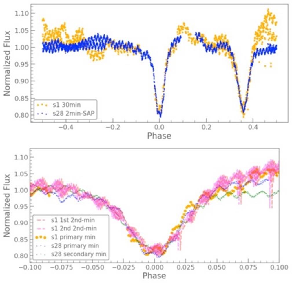
Fig. 21 Normalized TESS photometric data for Sectors 1 and 28 (s1, s28) showing the primary eclipse at phase= 0 and on top of the light curve folded with the period P = 19.2654 d. Clearly seen are the oscillations with a period of Posc = 0.25 d, observed at both eclipses of the Star A + Star B system. Upper pannel: Two secondary and one primary eclipse were observed in Sector 1 and one primary and one secondary were observed in Sector 28. Lower pannel: As above, but the abscissa gives the distance in orbital phase from mid-eclipse of the five eclipses. The color figure can be viewed online.
Then the brightness and emission line intensities declined reaching an apparent minimum in 2010-2013. The sudden outburst occurred in 1994, with a “precursor” in 1993, both prior to the maximum in the long term trend. We illustrate in Figure 20 the visual magnitude evolution of HD 5980 during the time frame 1987-2010. The complete light curve covering epochs 1950-2018 is presented in Figure 22.
Fig. 22 Same as Figure 20, but here containing all the historic photometric data available. The color figure can be viewed online.
One of the possible scenarios that might explain the long-term behavior is that Star A was undergoing an evolutionary transition making it brighter and more extended until it reached a critical radius at which the sudden outburst was triggered. If this were the case, however, it is not clear whether the loss of ≈ 10−3 M⊙ would have been sufficient to slow the expansion and then allow the star to contract once again to its current state. However, luminous blue variables (LBVs) are known to undergo cyclical changes that impact their photospheric and wind properties. If this were the case, then Star A would be the only know LBV with WR spectral spectral characteristics (except possibly the erupting variable in η Carinae).
An alternative interpretation is that the tidal shear energy dissipation in sub-surface Star A layers caused it to slowly expand until it reached a critical condition at which an external layer was ejected, thus liberating the accumulated energy. Tidal shear energy dissipation was shown to be a viable mechanism for bloating a star in the case of the red nova V1309 Sco (Koenigsberger & Moreno 2016). In the case of HD 5980, Toledano et al. (2007) outlined the manner in which an increasing stellar radius would lead to increasing tidal shear, eventually causing the eruption.
A more speculative possibility for the outbursts is that they could have been triggered by unstable accretion of Star A material onto Star B, as it has been proposed for the case of η Carinae (Soker & Behar 2006). Our observational results leave open the possibility that Star B may not be a typical WNE star. The observations indicate that, as Star A’s massloss rate increased, the WCZ emission also increased, implying a denser collision region. Hydrodynamical wind-wind collision studies show that when the wind momentum of one of the stars is significantly larger than that of its companion, a fraction of the shocked wind is accreted (Matsuda et al. 1992; Ruffert & Arnett 1994; Nagae et al. 2004). Under stationary conditions, the accretion rate is (probably) not sufficient to affect the secondary, but if the incoming stellar wind evolves over time becoming denser and slower, then the numerical simulations find that high density clumps produced by the instabilities in the shocks will fall onto the secondary star (Kashi 2020), potentially leading to non-negligible accretion rates. If such a phenomenon occurred in 1992-1994, the violent expulsion of the material accreted onto Star B could have been responsible for the transitory B1.5Ia+ spectrum observed in 1994 and the rapid spectral evolution of the system over the following two years. The persistent underlying WN spectrum at that time (Koenigsberger 2004) would in this case have been that of Star A.
7.6. Future Work
A treasure trove of information is encoded in the line profile variations. Future investigations could make use of the detailed variability of just a single line such as HeII 5411 to constrain the geometrical extent, general physical conditions, and velocity fields in the WCZ, but to do so requires the use of 3D radiative-hydrodynamic simulations and a densely packed (in orbital phase) set of observations over an entire orbital cycle. Though costly in observing time and computational resources, the expected outcome would include very valuable information on the structure of highly radiative shocks, and would yield a deeper understanding of the Star A + Star B interacting system.
Our new RV curves are consistent with those analyzed in Koenigsberger et al. (2014), and thus the derived masses are not expected to change with respect to those obtained previously. Also, the relative continuum luminosities are unaffected by our new results, so the conclusion that both objects are extremely massive and luminous still holds. A possible change lies in what is assumed for the evolutionary state of Star B. Its high luminosity suggests a chemically homogeneous evolutionary path (Koenigsberger et al. 2014). However, if it is not a WN star, then a potentially interesting (speculative) scenario is one in which mass transferred from Star A to Star B via unstable wind accretion has led to sequential violent ejections from Star B’s surface reducing its mass and prolonging its main sequence lifetime. Clearly, this conjecture requires the identification of an instability violent enough to eject the material from Star B’s surface and leave the system. The alternative conjecture, that Star A is the source of the 1993-1994 eruption, also requires further investigation, as no other WNh type star is known to have presented such a violent instability.
The properties of the “third light” source, Star C also merit further studies. Although a well-defined photospheric line spectrum is associated with one of the components in this highly eccentric (e ≈ 0.8, P C =96 d) system, there is no information as yet regarding the nature of its companion, nor whether it is gravitationally bound to the Star A + Star B system. Star C’s high eccentricity, line of sight coincidence to the Star A + Star B system, and brightness make it tempting to suggest that both binaries may be in a very wide orbit around each other.
Finally, it is also interesting to ponder the question of HD 5980’s apparent uniqueness. It may be so only because it is a massive eclipsing system that we have been lucky enough to catch in a very short-lived evolutionary state that many other systems already have or will experience. Given its location in the low-metallicity SMC environment, HD 5980 could be typical of many massive objects yet to be identified in distant extragalactic sources.