


 nova página do texto(beta)
 Inglês (pdf)
 Artigo em XML
 Referências do artigo
 Enviar este artigo por email
 Citado por SciELO
  Similares em
SciELO
Similares em
SciELO 
 Permalink
1. Introduction
Cen X-3 is an eclipsing high-mass X-ray binary system formed by an O-type donor star and a neutron star. Its complex X-ray behaviour makes both its temporal and spectral analysis extremely important to better understand its properties. So far, it is the only high-mass X-ray binary (HMXB) system in the Milky Way where mass transfer onto a neutron star occurs directly from the surface of the donor star (via Roche lobe overflow). The source was discovered in 1967 (Chodil et al. 1967) and Krzeminski (1974) estimated the distance as ≈ 8 kpc. The distance to Cen X-3 obtained from the European Space Agency (ESA) mission Gaia1 Early Data Release 3 (GEDR3) is d(kpc) =
It consists of a neutron star (NS) and a giant star O6-8 III companion called V779 Cen (Hutchings et al. 1979) with mass ≈ 20 M⊙ (van der Meer et al. 2007) and radius ≈ 12 R⊙ (Naik et al. 2011). Rawls et al. (2011) calculated the NS mass by using a Monte Carlo method and assuming a Roche lobe filling factor between 0.9 and 1.0, MNS = (1.35 ± 0.15) M⊙. However, applying another technique based on eclipsing light curve analysis and including an accretion disc around the NS, they derived a final mass for this system of (1.49 ± 0.08) M⊙. The binary orbit is almost circular, eccentricity e < 0.0016 (Bildsten et al. 1997), with an orbital period of ≈ 2.1 days, determined from regular X-ray eclipses (Schreier et al. 1972).
The observed average high X-ray emission ≈ 1037 erg s−1 compared to that observed in windfed accreting systems ≈ 1036 erg s−1 (Martinez-Núñez et al. 2017; Kretschmar et al. 2019) suggests additional structures in the NS environment. Studies of the light curve of Cen X-3 (Tjemkes et al. 1986) and the observed overall NS spin-up trend of 1.135 ms yr−1 with fluctuations on time scales of years (Tsunemi et al. 1996), together with the detection of quasi periodic oscillations (QPOs) from the source (Takeshima et al. 1991; Raichur & Paul 2008b) showed evidences of an accretion disk, due to Roche lobe overflow. Other structures such as an additional gas stream or an accretion wake might also be present in the accretion scenario in this source (Stevens 1988; Suchy et al. 2008).
Thus, variability of model parameters along the orbital phase allow us not only to investigate the characteristics of the circumstellar matter around the NS but also to trace permanent wind structures. Many authors have reported on the iron emission lines of Cen X-3 (Ebisawa et al. 1996; Iaria et al. 2005; Naik & Paul 2012; Rodes et al. 2017; Aftab et al. 2019) around the orbital period. Although MAXI was able to detect the Fe Kα, it cannot resolve it properly. However, changes in the central energy of the iron line with the orbital phase pointed to a coexistence of two iron lines at different energies (Rodes et al. 2017). Therefore, by using ASCA description of the iron emission lines of Cen X-3 we fitted three Gaussian profiles to the MAXI/GSC data, fixing some of the line parameters to estimate their equivalent widths.
In this paper we present the spectroscopic and light curve analysis of Cen X-3 observed with MAXI. MAXI / GSC data covers the entire orbit and extends over more than six years. Orbital phase-averaged and phase-resolved spectroscopy were performed applying several models in the 2-20 keV energy range. Observations and data reduction are described in § 2, timing analysis is presented in § 3, orbital phase-averaged spectrum and orbital phase-resolved spectra results are discussed in § 4, and § 5 contains the summary of the main findings.
2. Observations and Data
MAXI is an X-ray monitor on board the International Space Station (ISS) since August 2009 (Matsuoka et al. 2009). Every ≈ 92 minutes it scans almost the entire sky in each ISS orbit, observing a particular source for about 40 -150 s (Sugizaki et al. 2011) depending on the position of the object. It consists of two types of X-ray slit cameras, the Gas Slit Camera (GSC, Mihara et al. 2011) in the 2.0-20.0 keV, and the Solid-state Slit Camera (SSC, Tomida et al. 2011) operating in the 0.7-7.0 keV energy range. The in-orbit performance of GSC and SSC is presented in Sugizaki et al. (2011) and Tsunemi et al. (2010), respectively.
3. Timing Analysis
Firstly, we have extracted the MAXI/GSC on-demand light curves of Cen X-3 with a time resolution of one ISS orbit in five energy bands, 2.0- 20.0, 2.0-4.0, 4.0-10.0, 10.0-20.0 and 5.7-7.5 keV. To analyse the light curves we used Python and the Starlink software package2.
Secondly, we have used the Lomb-Scargle technique (Press & Rybicki 1989) to determine the orbital period from the original light curve 2.0-20.0 keV and have obtained Porb = 2.0870 ± 0.0005 days (Figure 2), which is comparable to that obtained by Nagase et al. (1992), Raichur & Paul (2010), Falanga et al. (2015) or Rodes et al. (2017). The errors in the periods were estimated using the Peaks tool inside the time-series analysis package Period in Starlink. The effect of the barycentric correction on the light curves was found to be negligible and did not need to be taken into consideration. Then, we folded the light curves with the best orbital period to produce energy-resolved orbital intensity profiles using the ephemeris from Falanga et al. (2015). In Table 1 we compiled the ephemeris data used for timing calculations.
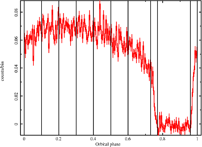
Fig. 1 Background subtracted light curve in 10.0-20.0 keV energy range. The color figure can be viewed online.

Fig. 2 Lomb-Scargle periodogram of the 2.0-20.0 keV light curve. The color figure can be viewed online.
Table 1 Ephemeris Data Used for Timing Calculations
| T0,ecl(MJD) | 50506.788423 ± 0.000007 |
| Porb (d) | 2.08704106 ± 0.00000003* |
| Ṗorb/Porb (10−6yr−1) | −1.800 ± 0.001 |
As a sample, the resulting orbital light curve between 10.0-20.0 keV is plotted in Figure 1 where the strongest changes are observed as the NS ingresses and egresses from eclipse. We defined ten orbital phase bins corresponding to phase intervals [0.0-0.1] (post-egress), [0.1-0.2], [0.2-0.3], [0.3-0.4], [0.4-0.5], [0.5-0.6], [0.6-0.73] (pre-ingress), [0.73-0.77] (ingress), [0.77-0.96] (which corresponds to the total eclipse) and [0.96-1.0] (egress).
Another two maximum peaks were present in the Lomb-Scargle periodogram. The first one with a power of 430.03 corresponds to a period of 220 ± 5 days, which might be consistent with the superorbital period of 93.3-435.1 days reported by Sugimoto et al. (2014). The second one with a power of 422.48 corresponds to a period of ≈ 1.04 days, which is a harmonic of the orbital period. In addition, around the superorbital period, there are a few more peaks that can be interpreted as QPOs (Figure 3), as also pointed out by Raichur & Paul (2008a), Raichur & Paul (2008b), Takeshima et al. (1991) and Priedhorsky & Terrell (1983).

Fig. 3 Zoom of the QPOs in the original 2.0-20.0 keV light curve. The color figure can be viewed online.
It is expected that HMXBs show strong absorption at low energies (below 4 keV), complex iron emission lines between 6.4 keV and 7.2 keV and an energy cutoff at high energies (greater than 10 keV). In order to analyse the light curves variability the MAXI/GSC energy range (2.0-20.0 keV) has been divided into 2.0-4.0 keV (low energy), 4.0-10.0 keV (medium energy), 5.7-7.5 keV (iron complex emission lines) and 10.0-20.0 keV (high energy) bands. Therefore, we have calculated the hardness ratio defined as H/S, where H are the net counts in the hard band and S are those obtained in the soft band, between the light curves: (5.7-7.5 keV) / (2.0-4.0 keV), (4.0-10.0 keV) / (5.7-7.5 keV), (10.0-20.0 keV) / (5.7-7.5 keV), (10.0-20.0 keV) / (2.0-4.0 keV), (10.0-20.0 keV) / (4.0-10.0 keV) and (4.0-10.0 keV) / (2.0-4.0 keV).
From the folded light curve, the hardness ratio measurements obtained for each pointing along the orbit had large error bars. Therefore, they were averaged over 150 points and the uncertainties were estimated using error propagation. The overall profile shape was quite similar and consistent with a constant value, so we could not identify any morphology or tendency (see Figure 4, top panel). Figure 4, bottom panel, shows the hardness ratio using a weighted average over 150 bins. The hardness ratio is consistent with a constant (HR ≈ 0.75) for the out of eclipse indicating there is no significant change in the spectral shape. On the other hand, during the eclipse the brightness of Cen X-3 is also consistent with a constant value (HR ≈ 0.3) but 2.5 times lower than out of eclipse. Both the drop in brightness at eclipse ingress and the rise in brightness at eclipse egress are quite sharp.
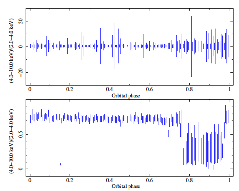
Fig. 4 Hardness ratio H/S = (4.0 − 10.0 keV)/(2.0 − 4.0 keV). Top panel: using simple average. Bottom panel: using weighted average. The color figure can be viewed online.
The process to obtain the hardness curves (H S)/(H + S) is the same used to calculate H/S, where H = 4.0-10.0 keV and S = 2.0-4.0 keV (Figure 5). The general trend of the hardness curve is very similar to that of the hardness ratio, although the decrease and increase before and after the eclipse is smoother. Moreover, as can be seen in Figures 14 (equation 2) and 15 (equation 5) it is consistent with the behaviour of the unabsorbed flux variation.

Fig. 5 Hardness curve (H − S)/(H + S) using weighted average, where H = 4.0 − 10.0 keV and S = 2.0 − 4.0 keV energy bands. The color figure can be viewed online.
During an orbital period of Cen X-3, MAXI/GSC can perform up to 33 observations of the object (an example is shown in Figure 6). However, for individual point X-ray sources, the MAXI/GSC detector has very short exposures of about 60 s fifteen times a day which is not long enough to extract orbital phase-resolved spectra. As a consequence, it is necessary to accumulate observations in each orbital phase to obtain spectra with a good signal-to-noise ratio.

4. Spectral Analysis
4.1. Orbital Phase Averaged Spectrum
We have extracted the orbital phase averaged spectrum of Cen X-3 (see Figure 7) with MAXI/GSC using the MAXI on-demand processing3, carefully excluding any contamination by nearby brighter sources. For spectral analysis we used the XSPEC fitting package, released as a part of XANADU in the HEASoft tools. We tested both phenomenological and physical models commonly applied to accreting X-ray pulsars and rebinned all extracted spectra to obtain spectral bins by Gaussian distribution.
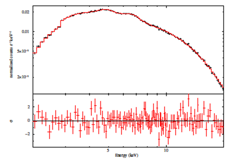
Fig. 7 Orbital phase averaged spectrum of Cen X-3 in the 2.0-20.0 keV band. Top panel: data and best-fit model described by equation (2). Bottom panel: residuals between the spectrum and the model. The resulting fit parameters are reported in Table 2. The color figure can be viewed online.
Absorbed Comptonisation models have been successfully applied to HMXBs in the 2.0-20.0 keV energy range covered by MAXI/GSC, such as Vela X-1 (Doroshenko et al. 2013), 4U 1538-52 (Rodes-Roca et al. 2015) and Cen X-3 (Rodes et al. 2017). We started to describe the orbital phase-averaged spectrum using a simple partial absorbed Comptonisation model modified by a Gaussian absorption line at 5 keV to compensate the incompleteness of the MAXI/GSC response (Nakahira private communication). An iron fluorescence emission line present in the spectrum is modelled with a Gaussian component, Fe Kα at 6.4 keV. This model is described by equation (1).
where, in terms of XSPEC, pcfabs is a partial covering fraction absorption that affects only a fraction f of the model component multiplied by it, gabs is the Gaussian absorption line component, compST is the Comptonisation of cool photons on hot electrons (Sunyaev & Titarchuk 1980), and the Gaussian line is added to describe the Fe Kα line. The absorption cross sections were taken from Verner & Yakovlev (1995) and the abundances were set to those of Wilms et al. (2000).
Although this model describes the averaged spectra between 2.0-20.0 keV well (χr2 = 1.09), it cannot offer a good statistical and/or physical solution for all orbital phase-resolved spectra. For example, fitting the eclipse spectrum, i.e. when the direct X-ray emission is totally blocked by the companion, we obtained that the covering fraction factor was f ≈ 0. Model parameters were also not well constrained. As the aim was to satisfactorily describe both the aver aged spectrum and the orbital phase-resolved spectra with the same model, it was decided to reject it.
Recently, Aftab et al. (2019) and Sanjurjo-Ferrín et al. (2021) carried out spectral analysis of XMM-Newton data in the eclipse and out-of-eclipse phases in the energy band (0.8-10.0 keV). They obtained best fits by combining blackbody and power-law components and used them to describe both eclipse and out-of-eclipse spectra. In addition, Wojdowski et al. (2001) argued that the stellar wind in the system is smooth and concluded that the wind is most likely driven by X-ray heating of the illuminated surface of the companion star as proposed by Day & Stevens (1993). Compared to previous studies, thanks to MAXI/GSC’s observation strategy, a large number of complete orbits have been observed and divided into 10 orbital phase intervals. According to the previous discussion, finally, models including either a blackbody component (bbody in XSPEC) or a Comptonisation component (compST in XSPEC) have been combined to describe the average spectrum.
Interstellar medium (ISM) absorption and local absorption components have been included by means of a partial covering fraction defined through the parameter C. The tbnew4 component is a recent version of the Tübingen-Boulder absorption model which updates the absorption cross sections and abundances (Wilms et al. 2000); the gabs factor has been described above; po is a simple photon power law consisting of a dimensionless photon index (Γ) and the normalisation constant (K), the spectral photons keV−1 cm−2 s−1 at 1 keV; bbody corresponds to a blackbody model whose parameters include the temperature kTbb in keV and the normalisation norm, defined as L39/D2, where L39 is the source luminosity in units of 1039 erg s−1 and D2 is the distance to the source in units of 10 kpc. This model is given by equation (2).
where GL represents the Gaussian functions added to account for the emission lines. Here, parameters derived from ASCA data by Ebisawa et al. (1996) were used to describe the Fe Kα complex.
Fitted parameters for the continuum model are listed in Table 2 where it is also included the equivalent width (EW) of the Gaussian emission lines. Figure 7 shows the data, the best-fit model described by equation (2), and residuals as the difference between observed flux and model flux divided by the uncertainty of the observed flux.
Table 2 Best-Fit Model Parameters for the Averaged Spectruma
| Component | Parameter | Value |
|---|---|---|
| P.c.f. | C | 0.71 ± 0.08 |
| tbnew | N1H [1022 atoms cm-2] | 19+4-3 |
| N2H [1022 atoms cm-2 | 2.5+6-0.5 | |
| gasb | E[keV] | 5.12 ± 0.05 |
| σ [keV] | 0.02 (frozen) | |
| line depth | 0.7+0.14-0.4 | |
| Power law | Photon index Γ | 2.16 ± 0.15 |
| norm [keV-1 s-1 cm-2] | 0.44+0.14-0.11 | |
| body | kT [keV] | 3.46 ± 0.04 |
| norm [L39 / D210] | 0.0171+0.0021-0.0018 | |
| Fe Kα | Line E[keV] | 6.42 (frozen) |
| σ [keV] | 0.01 (frozen) | |
| EW [keV] | 0.023 ± 0.004 | |
| norm [10-4 ph s-1 cm-2] | 8.0 ± 1.13 | |
| Fe XXV | Line E[keV] | 6.69 (frozen) |
| σ[keV] | 0.01 (frozen) | |
| EW [keV] | 0.025 ± 0.004 | |
| norm [10-4 ph s-1 cm-2] | 8.4 ± 1.3 | |
| Fe XXVI | Line E[keV] | 6.99 (frozen) |
| σ[keV] | 0.01 (frozen) | |
| EW [keV] | 0.025 ± 0.004 | |
| norm [10-4 ph s-1 cm-2] | 8.4 ± 1.3 | |
| Χ2r | Χ2r / (d.o.f.)=115 / 106 = 1.1 | |
aParameters for equation (2). P.c.f. is the partial covering fraction. EW represents the equivalent width of the emission line. Uncertainties are given at the 90% (∆χ2 = 2.71) confidence limit and d.o.f is degrees of freedom.
Since the surface luminosity of a blackbody only depends on its temperature, it is possible to calculate the radius of the emitting region, Rbb, by using the expression:
where D is the distance to the source in kpc, Fbb is the unabsorbed flux in erg s-1 cm-2 in the energy range 2.0-20.0 keV, Tbb the temperature in keV. Taking into account the distance to the source given by GAIA (E)DR3 d(kpc) =
The intrinsic bolometric X-ray luminosity is a key parameter to infer the stellar wind parameters and the details of the accretion processes. It is usually estimated from the measured X-ray flux of the source by using equation (4). Although the accretion flow is not expected to be as isotropic as the stellar wind, here, it is assumed that the system is emitting isotropically. A few cautions should be kept in mind when using this assumption: in accreting neutron stars, the bulk of the x-rays are produced in the accretion columns near the two magnetic poles; the emission profiles of these regions are not well known; the bolometric flux is measured on a small energy band and derived from phenomenological rather than physically justified models (see Martínez-Núñez et al. (2017) for a review of stellar winds from massive stars).
where LX is the X-ray luminosity, D is the distance to the source and ƒno_abs is the unabsorbed flux in the 2.0-20.0 keV energy band. We obtained LX =
From the bbody normalization, L39 / D210, a value of
Another model has been also tested by replacing the blackbody by a Comptonisation model, maintaining the rest of the components unchanged. This model is described by equation (5).
Best-fit model parameters are listed in Table 3 and Figure 8 shows the averaged spectrum. From the model, the inferred unabsorbed flux was (3+6-1) × 10−9 erg s−1 cm−2 in the MAXI/GSC energy band, corresponding to an X-ray luminosity of LX = (2+3-1) × 1037 erg s−1 which agrees completely with the previous result.
Table 3 Best-Fit Model Parameters for the Averaged Spectruma
| Component | Parameter | Value |
|---|---|---|
| P.c.f. | C | 0.80+0.09-0.08 |
| tbnew | N1H [1022 atoms cm-2] | 15+4-3 |
| N2H [1022 atoms cm-2 | 1.9+6-0.5 | |
| gabs | E[keV] | 5.12 ± 0.05 |
| σ [keV] | 0.02 (frozen) | |
| line depth | 0.5+0.8-0.3 | |
| Power law | Γ | 2.6+0.8-0.5 |
| norm [keV-1 s-1 cm-2] | 0.3+0.05-0.1 | |
| compST | kT [keV] | 3.935 ± 0.009 |
| τ | 18.6+0.08-1.0 | |
| norm | 0.08+0.03-0.02 | |
| Fe Kα | Line E[keV] | 6.42 (frozen) |
| σ [keV] | 0.01 (frozen) | |
| EW [keV] | 0.035 ± 0.004 | |
| norm [10-3 ph s-1 cm-2] | 1.05 ± 0.11 | |
| Fe XXV | Line E[keV] | 6.69 (frozen) |
| σ [keV] | 0.01 (frozen) | |
| EW [keV] | 0.016 ± 0.004 | |
| norm [10-4 ph s-1 cm-2] | 4.8 ± 1.1 | |
| Fe XXVI | Line E[keV] | 6.99 (frozen) |
| σ[keV] | 0.01 (frozen) | |
| EW [keV] | 0.021 ± 0.004 | |
| norm [10-4 ph s-1 cm-2] | 5.2 ± 1.1 | |
| Χ2r | Χ2r / (d.o.f.)=115 / 106 = 1.1 | |
aParameters for equation (5). P.c.f. is the partial covering fraction. EW represents the equivalent width of the emission line. Uncertainties are given at the 90% confidence limit and d.o.f is degrees of freedom.

Fig. 8 Orbital phase averaged spectra of Cen X-3 in the 2.0-20.0 keV band. Top panel: data and best-fit model (equation (5)). Bottom panel: residuals between the spectrum and the model. The resulting fit parameters are reported in Table 3. The color figure can be viewed online.
The Comptonisation parameter y = kTτ2 / (me c2), where k is the Boltzmann constant, T is the temperature, τ is the optical depth, me is the electron mass and c is the light speed, determines the efficiency of the Comptonisation process (Titarchuk 1994; Prat et al. 2008), and its value from the averaged spectrum y =
The iron fluorescence emission line shows an interesting evolution along the orbital phase: it is centred at 6.4 keV out-of-eclipse but it is shifted to 6.7 keV at the ingress suggesting the coexistence of two iron lines at different energies (Rodes et al. 2017). Sensitive X-ray observatories such as ASCA and XMM-Newton have detected and resolved the Fe complex in Cen X-3 (Ebisawa et al. 1996; Sanjurjo-Ferrín et al. 2021, respectively). In contrast, MAXI/GSC is not able to resolve it and therefore the values obtained for these lines by Ebisawa et al. (1996) have been used to fit them. For this purpose, all their parameters except the line intensities were fixed (see Tables 2 and 3). The line flux ratio [Fe XXVI] / [Fe XXV] can be used to estimate the ionisation state of the emitting plasma.
The results obtained in the averaged spectrum for both models were 0.6 ± 0.3 (equation 2) and 1.1 ± 0.5 (equation 5), respectively. Assuming that this procedure is an approximation of the ionisation state of the system, these average values point to a highly ionised plasma with log ξ ≈ (3.4 - 3.8), according to the ionisation parameter calculated by Ebisawa et al. (1996, their Figure 8, upper panel).
Since the partial covering fraction modifies the continuum at low energies, two hydrogen column components were applied: one to describe the ISM towards the system, N2H, and the other to describe the ISM plus local absorption, N1H. The mean value of the Galactic column density of hydrogen NH,tot in the direction of Cen X-3 is 1.16 × 1022 cm−2 (Willingale et al. 2013). Valencic & Smith (2015) reported an ISM absorption towards this source of (1.6 ± 0.3) × 1022 cm−2. The column N2 derived from both models are compatible taking into account its uncertainties.
4.2. Orbital Phase Averaged, High and Low States Spectra with MAXI/GSC
As a consequence of the large variability of the light curve, high and low states have been defined. Thus, the good time intervals (GTIs) of both states have been identified in the energy range 2.0-20.0 keV and their respective averaged spectra have been extracted. In this analysis, we fitted the high and low states spectra with the same models as we used in the orbital phase-averaged spectrum, except that only a single here. Gaussian has been included The fits are shown in Figures 9 and 10; meanwhile, the best-fit model parameters are listed in Tables 4 (equation 2) and 5 (equation 5).
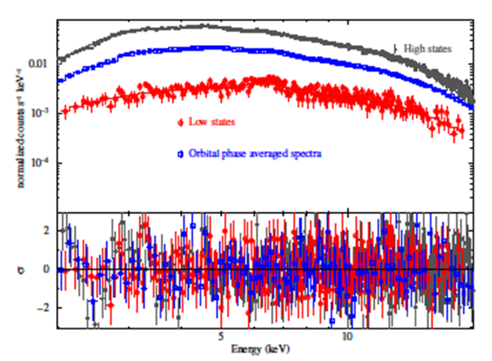
Fig. 9 Orbital phase averaged, high states and low states spectra of Cen X-3 in the 2.0-20.0 keV band. Top panel: Data and best-fit models defined by equation (2). Bottom panel: residuals for the model. The resulting fit parameters are reported in Table 4. The color figure can be viewed online.
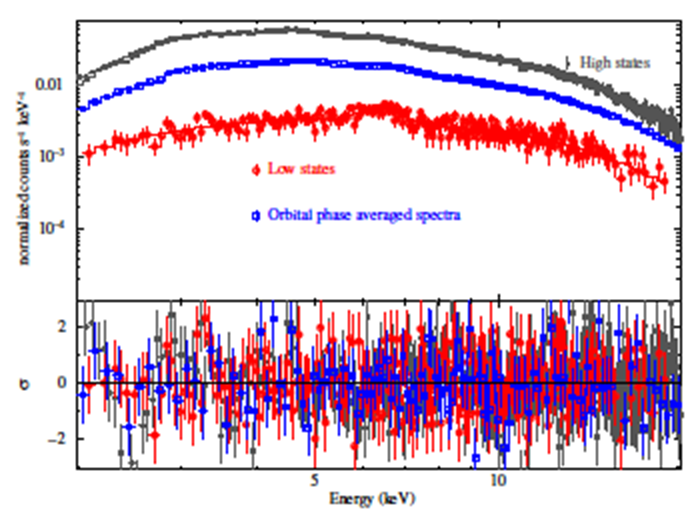
Fig. 10 Orbital phase averaged, high states and low states spectra of Cen X-3 in the 2.0-20.0 keV band. Top panel: Data and best-fit models defined by equation (5). Bottom panel: residuals for the model. The resulting fit parameters are reported in Table 5. The color figure can be viewed online.
To determine the periods of high and low activity we established a number of counts greater than ≈ 0.5 photons s−1 cm−2 and less than ≈ 0.3 photons s−1 cm−2, respectively. Then, more than 100 bins (one bin ≈ 0.1 MJD) were accumulated to calculate the low-activity intervals and grouped 10 bins by 10 bins for the high-activity events.
The unabsorbed fluxes of the orbital phase-averaged, high and low activity spectra in units of erg s−1cm−2 are (1.72 ± 0.03) × 10−9, (4.1+1.3) × 10−9 and (5.4+1.5−1.2) × 10-10, respectively. For such fluxes, the radius of the blackbody emitting area is found Rbb = 0.71+0.07-0.06 km (averaged spectra), Rbb = 1.6 ± 0.5 km (high states) and Rbb = 0.36+0.12−0.10 km (low states). All values are on the order of 1 to 2 km which is compatible with a hot spot on the NS surface (Sanjurjo-Ferrín et al. 2021).
Using the definition of the bbody normalization, L39/D210, we have derived its value in the three spectra: 0.04+0.08−0.07 (averaged spectra), 0.1 ± 0.3 (high states) and 0.009+0.019−0.016 (low states). These values are consistent with the experimental ones, taking the uncertainties into account (see Table 4).
Table 4 Best-Fit Model Parameters For The Averaged, High States And Low States Spectraa
| Component | Parameter | Value |
|---|---|---|
| P.c.f. | C | 0.809 ± 0.003 |
| tbnew | N1H [1022 atoms cm-2] | 18.8 ± 0.06 |
| N2H [1022 atoms cm-2] | 2.57 ± 0.07 | |
| gabs | E[keV] | 5.12 (frozen) |
| σ [keV] | 0.02 (frozen) | |
| line depth | 0.7 (frozen) | |
| Power law | Γ | 2.184 ± 0.009 |
| norm [keV-1 s-1 cm-2] | 0.405 ± 0.006 | |
| bbody | kT [keV] | 3.4628 ± 0.0023 |
| norm [L39 / D210] | 0.01527 ± 0.00014 | |
| Fe Kα | Line E[keV] | 6.67 ± 0.05 |
| σ [keV] | 0.28+0.07-0.08 | |
| EW [keV] | 0.070 ± 0.004 | |
| norm [10-3 ph s-1 cm-2] | 1.98 ± 0.12 | |
| Χ2r | Χ2r / (d.o.f.)=115 / 108 = 1.1 | |
| P.c.f. | C | 0.800 ± 0.003 |
| tbnew | N1H [1022 atoms cm-2] | 63+17-11 |
| N2H [1022 atoms cm-2] | 6.9 ± 0.05 | |
| gabs | E[keV] | 5.12 (frozen) |
| σ [keV] | 0.02 (frozen) | |
| line depth | 0.07 (frozen) | |
| Power law | Γ | 2.65+0.22-0.21 |
| norm [keV-1 s-1 cm-2] | 3.8+1.2-0.9 | |
| bbody | kT [keV] | 2.87+0.09-0.18 |
| norm [L39 / D2 10] | 0.033 ± 0.004 | |
| Χ2r | Χ2r / (d.o.f.) = 452 / 351 = 1.3 | |
| P.c.f. | C | 0.80 ± 0.03 |
| tbnew | N1H [1022 atoms cm-2] | 18+7-5 |
| N2H [1022 atoms cm-2] | 1.4+0.09-0.07 | |
| gabs | E[keV] | 5.12 (frozen) |
| σ [keV] | 0.02 (frozen) | |
| line depth | 0.69 (frozen) | |
| Power law | Γ | 2.55 ± 0.018 |
| norm [keV-1 s-1 cm-2] | 0.071+0.020-0.016 | |
| bbody | kT [keV] | 3.67+0.18-0.17 |
| norm [L39 / D2 10] | 0.0050+0.0004-0.0003 | |
| Fe Kα | Line E[keV] | 6.31 ± 0.10 |
| σ [keV] | 0.22+0.19-0.22 | |
| EW [keV] | 0.22 ± 0.04 | |
| norm [10-3 ph s-1 cm-2] | 1.6 ± 0. | |
| Χ2r | Χ2r / (d.o.f.) = 206 / 220 = 0.9 | |
aParameters for equation (2). P.c.f. is the partial covering fraction. EW represents the equivalent width of the emission line. Uncertainties are given at the 90% confidence limit and d.o.f is degrees of freedom.
The Comptonisation parameter y (see Table 6) shows an efficient process that corresponds to a moderate accretion rate if we take into account the uncertainties.
Table 5 Best-Fit Model Parameters for the Averaged, High States And Low States Spectraa
| Component | Parameter | Value |
|---|---|---|
| P.c.f. | C | 0.813 ± 0.004 |
| tbnew | N1H [1022 atoms cm-2] | 15.9 ± 0.05 |
| N2H [1022 atoms cm-2] | 2.22 ± 0.08 | |
| gabs | E[keV] | 5.12 (frozen) |
| σ [keV] | 0.02 (frozen) | |
| line depth | 0.5 (frozen) | |
| Power law | Γ | 2.612 ± 0.023 |
| norm [keV-1 s-1 cm-2] | 0.323 ± 0.011 | |
| compST | kT [keV] | 3.90 ± 0.04 |
| τ | 19.26+0.24-0.23 | |
| norm | 0.0709 ± 0.013 | |
| Fe Kα | Line E[keV] | 6.65 ± 0.04 |
| σ [keV] | 0.28 ± 0.07 | |
| EW [keV] | 0.074 ± 0.004 | |
| norm [10-3 ph s-1 cm-2] | 2.04 ± 0.12 | |
| Χ2r | Χ2r / (d.o.f.)=111 / 107 = 1.0 | |
| P.c.f. | C | 0.840+0.012-0.11 |
| tbnew | N1H [1022 atoms cm-2] | 66+4-3 |
| N2H [1022 atoms cm-2] | 6.87+0.12-0.11 | |
| gabs | E[keV] | 5.12 (frozen) |
| σ [keV] | 0.02 (frozen) | |
| line depth | 0.05 (frozen) | |
| Power law | Γ | 2.603±0.012 |
| norm [keV-1 s-1 cm-2] | 3.42 ± 0.07 | |
| compST | kT [keV] | 2.85±0.005 |
| τ | 48+8-6 | |
| norm | 0.23+0.006-0.005 | |
| Χ2r | Χ2r / (d.o.f.) = 452 / 350 = 1.3 | |
| P.c.f. | C | 0.80+0.04-0.03 |
| tbnew | N1H [1022 atoms cm-2] | 18+7-5 |
| N2H [1022 atoms cm-2] | 1.1+0.9-0.7 | |
| gabs | E[keV] | 5.12 (frozen) |
| σ [keV] | 0.02 (frozen) | |
| line depth | 0.5 (frozen) | |
| Power law | Γ | 2.37 ± 0.17 |
| norm [keV-1 s-1 cm-2] | 0.055+0.015-0.012 | |
| compST | kT [keV] | 3.7 ± 0.03 |
| Τ | 43+22-9 | |
| Norm | 0.0026+0.0014-0.0013 | |
| Fe Kα | Line E[keV] | 6.31 ± 0.10 |
| σ [keV] | 0.22+0.17-0.22 | |
| EW [keV] | 0.22 ± 0.03 | |
| norm [10-3 ph s-1 cm-2] | 1.61±0.23 | |
| Χ2r | Χ2r / (d.o.f.) = 206 / 219 = 0.9 | |
aParameters for equation (2). P.c.f. is the partial covering fraction. EW represents the equivalent width of the emission line. Uncertainties are given at the 90% confidence limit and d.o.f is degrees of freedom.
Table 6 X-Ray Luminosity (1037 ERG S−1) and Comptonisation Parameter
| Orbital phase | Lx (equation 2) | Lx (equation 5) | y = k Tτ2/(me c2) |
|---|---|---|---|
| Averaged | 1.9+0.4-0.3 | 1.9+0.4-0.3 | 2.83 ± 0.10 |
| High states | 6.3 ± | 6.3+1.3-1.0 | 13+5-3 |
| Low states | 0.40+0.18-0.15 | 0.40+0.18-0.15 | 13+15-7 |
During the high state, when LX is close to 1038 erg s−1, the Fe Kα is not present in the spectrum. Moreover, the EW of the Fe Kα is three times higher during the low states than that in the averaged spectra. These facts suggest that the strong x-ray radiation may mask the possible presence of iron emission lines.
The unabsorbed flux is found to vary with a similar trend for both models. In fact, the X-ray luminosity is the same, taking the uncertainties into account (see Table 6, Column 2 corresponds to equation 2 and Column 3 corresponds to equation 5). On the one hand, it indicates (for averaged spectra and high states) that the accretion mode is not only due to the stellar wind (> 1036 erg s−1) but should also be enhanced by disk accretion or gas stream accretion. On the other hand, the luminosity indicates that the accretion mode in low states spectra is due to stellar wind. Therefore, the difference in X-ray luminosity between the high and low states can be attributed to a decrease in the accretion rate rather than an overall rise in absorption.
Tables 7 and 8 show the unabsorbed flux and the luminosity of each model component (equations 2 and 5, respectively) as well as the total unabsorbed fluxes and luminosities whose values agree with those given in Table 6.
Table 7 Unabsorbed Flux (10−9 ERG S−1 Cm−2) and Luminosity (1037 Erg S−1)*
| Component | Unabs. flux (equation 2) | LX (equation 2) |
|---|---|---|
| Power law | 1.72 ± 0.03 | 0.95+0.19-0.15 |
| bbody | 1.72 ± 0.03 | 0.95+0.19-0.15 |
| Fe Kα | 0.0343 ± 0.0005 | 0.019+0.004-0.003 |
| Total | 3.47 ± 0.06 | 1.9+0.4-0.3 |
| Power law | 7.3+2.3-1.7 | 4.1 ± 2.0 |
| bbody | 4.1+1.3-1.0 | 2.2+1.1-0.9 |
| Total | 11+4-3 | 6 ± 3 |
| Power law | 0.16 ± 0.04 | 0.9+0.04-0.03 |
| bbody | 0.54+0.15-0.12 | 0.30+0.14-0.11 |
| Fe Kα | 0.26+0.007-0.006 | 0.014+0.007-0.005 |
| Total | 0.73+0.20-0.17 | 0.40+0.19-0.15 |
*For the model components for the averaged, high states and low states spectra.
Table 8 Unabsorbed Flux (10−9 erg s−1 cm−2) And Luminosity (1037 erg s−1)*
| Component | Unabs. flux (equation 5) | LX (equation 5) |
|---|---|---|
| Power law | 0.676 ± 0.023 | 0.37+0.08-0.07 |
| compST | 2.67 ± 0.09 | 1.5 ± 0.3 |
| Fe Kα | 0.0353 ± 0.0012 | 0.020+0.004-0.003 |
| Total | 3.38 ± 0.11 | 1.9 ± 0.4 |
| Power law | 7.49 ± 0.15 | 4.2+0.8-0.7 |
| compST | 3.94 ± 0.08 | 2.2 ± 0.4 |
| Total | 11.43 ± 0.023 | 6.4+1.2-1.1 |
| Power law | 0.17+0.05-0.04 | 0.29+0.13-0.10 |
| compST | 0.52+0.14-0.11 | 0.30+0.14-0.11 |
| Fe Kα | 0.26+0.007-0.006 | 0.014+0.007-0.005 |
| Total | 0.72+0.20-0.17 | 0.39+0.18-0.14 |
*For the model components for the averaged, high states and low states spectra.
4.3 Orbital Phase-Resolved Spectra with MAXI/GSC
Previous studies following this direction of analysis have been performed in one or two orbits (Nagase et al. 1992; Suchy et al. 2008) or over shorter orbital phases (Ebisawa et al. 1996; Audley et al. 1996; Wojdowski et al. 2001; Aftab et al. 2019; Sanjurjo-Ferrín et al. 2021). We have obtained orbital phase-resolved spectra of the HMXB pulsar Cen X-3, accumulating the 60 s duration scans into ten orbital phase bins covering entirely its orbit (Rodes-Roca et al. 2015).
Based on the results from § 4.1, we fitted the orbital phase-resolved spectra with the same two models as we used in the orbital phase-averaged spectrum. Both models gave acceptable fits to observational data and the results are shown in Figures 11 and 12 for selected orbital phase-resolved spectra.

Fig. 11 Orbital phase-resolved spectra of Cen X-3 in the 2.0-20.0 keV band. Top panel: Selected spectra and best-fit models defined by equation (2). Bottom panel: residuals for the model. The color figure can be viewed online.

Fig. 12 Orbital phase-resolved spectra of Cen X-3 in the 2.0-20.0 keV band. Top panel: Selected spectra and best-fit models (defined by equation (5)). Bottom panel: residuals for the model. The color figure can be viewed online.
The degeneracy between the properties of the accretion rate and the physical parameters of the NS in all available models produces a certain degree of degeneracy between fit parameters. The behaviour of different parameters of the model described by equation (5) towards eclipse suggests degeneracies between them. To better explore the photon index variation, we constrained its value to the interval obtained between orbital phase 0.0 to 0.6, i.e. 1.90 < Γ < 2.85, and fitted the spectra of pre-ingress, ingress, eclipse and egress orbital phases again. The errors were obtained with the error task, provided by XSPEC, and with propagation of uncertainties. The new values obtained by this procedure differed only slightly from the previous values within errors. However, the photon index was not well constrained and exhibited relatively large errors. Our results are marked with open blue circles in Figures 14-18 and 20, where filled red squares represent the initial parameter values. The possible degeneracy between the spectral photon index Γ and absorption spectral parameters is known. Therefore, we produced χ2 contour plots of Γ and N1H for both models (see Figure 13). It is clear from this figure that the value of N 1 is moderately correlated to that of Γ as expected. However, the narrow energy band of MAXI/GSC as well as the observational mode makes it extremely difficult to remove this degeneracy through spectral fitting. In the following, we discuss the orbital phase spectral variation of the model parameters described by equations (2) and (5).
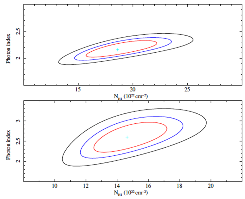
Fig. 13 The ellipses are χ2-contours for two parameters (N1H and Γ). The contours are 68%, 90% and 99% confidence levels for two interesting parameters. Top panel: averaged spectrum fitted by equation (2). Bottom panel: averaged spectrum fitted by equation (5). The color figure can be viewed online.
In Figures 14-18 and 20-21, we show the evolution of the relevant parameters of both models throughout orbital phase. The temperature of the blackbody is almost constant, decreasing drastically in the eclipse and increasing in the eclipse-egress. That implies that the emission zone of this component should be large. The normalisation of the black-body component shows a smooth decrease, which could be compatible with a constant value, reaching the minimum value at eclipse (Figure 14). The radius of the emission zone is of the order of 1 to 3 km whereas in eclipse it is about 9 ± 3 km (Figure 14). This fact could suggest soft X-ray reflection from the inner accretion disk region and agree with that reported by Sanjurjo-Ferrín et al. (2021).
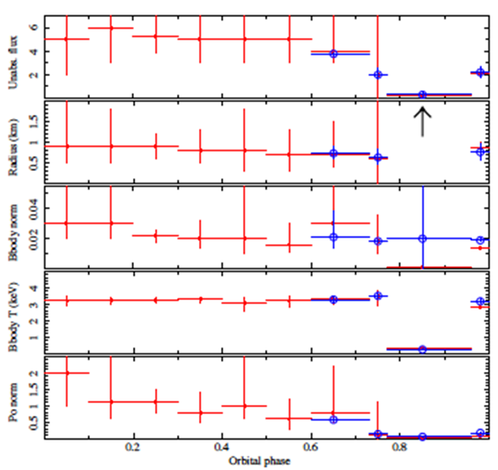
Fig. 14 Evolution of some parameters of the model described by equation (2). Unabsorbed flux is in units of 10−9 erg cm−2 s−1. Bbody norm is in units of L39/D210. Power-law normalization is expressed in units of keV−1 s−1 cm−2. Filled red squares: initial values. Open blue circles: values obtained by constraining the range of values of the photon index (pre-ingress, ingress, eclipse and egress). The color figure can be viewed online.

Fig. 15 Evolution of some parameters of the model described by equation (5). Unabsorbed flux is in units of 10−9 erg cm−2 s−1. Power-law normalisation is expressed in units of keV−1 s−1 cm−2. Filled red squares: initial values. Open blue circles: values obtained by constraining the range of values of the photon index (preingress, ingress, eclipse and egress). The color figure can be viewed online.
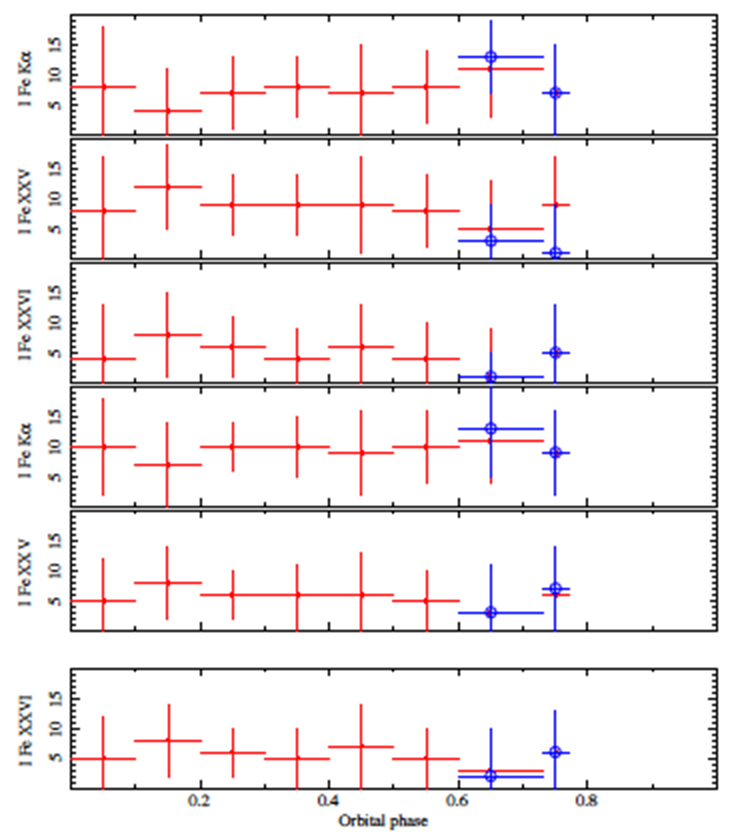
Fig. 16 Evolution of the Gaussian intensity of the Fe emission lines with orbital phase. Top, second and third panels: model described by equation (2). Fourth, fifth and bottom panels: model described by equation (5). The unit of the line flux I is 10−4 photons s−1 cm−2. Filled red squares: initial values. Open blue circles: values obtained by constraining the range of values of the photon index (pre-ingress, ingress, eclipse and egress). The color figure can be viewed online.

Fig. 17 Evolution of the equivalent width (EW) of the Fe emission lines with orbital phase. Top, second and third panels: model described by equation (2). Fourth, fifth and bottom panels: model described by equation (5). EW is in units of keV. Filled red squares: initial values. Open blue circles: values obtained by constraining the range of values of the photon index (pre-ingress, ingress, eclipse and egress). The color figure can be viewed online.

Fig. 18 Evolution of the partial covering fraction C and line intensity ratio Fe XXVI/Fe XXV. Top and second panels: model described by equation (2). Third and bottom panels: model described by equation (5). Filled red squares: initial values. Open blue circles: values obtained by constraining the range of values of the photon index (pre-ingress, ingress, eclipse and egress). The color figure can be viewed online.
When the neutron star is embedded into the stellar wind of the donor, the hydrogen column density shows a modulation along the orbit. Therefore, besides the interstellar medium absorption component (consistent with a constant value), we also allowed for the presence of a local absorber, modulated by a partial covering fraction that acts as a proxy for some features of the stellar wind of the donor star or the surroundings of the compact object.
For the model defined by equation (2), the normalisation of the power law decreases smoothly during out-of-eclipse before reaching a minimum during pre-eclipse, eclipse and eclipse-egress (Figure 14). The power-law photon index is rather stable during all orbital phases (Γ ≈ 2.1), but it drops to ≈ 1.3 in the eclipse-egress ([0.96-1.0]) (Figure 20, top panel).
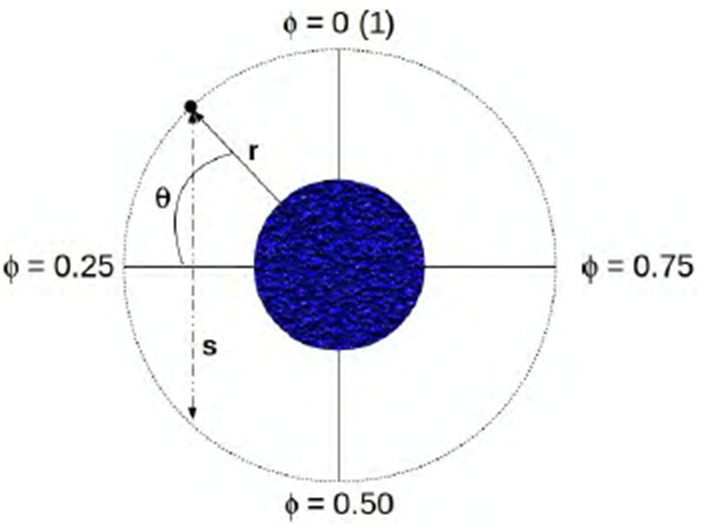
Fig. 19 Schematic view of the binary system. For simplicity we have assumed a circular orbit whose parameters r, s and θ are shown. We note that in this sketch the orbital phase 0 (1) is centred on the mid-time of eclipse. The color figure can be viewed online.

Fig. 20 Evolution of the photon index Γ and absorption columns N1H and N2H. Top, second and third panels: from equation (2). Fourth, fifth and bottom panels: from equation (5). Filled red squares: initial values. Open blue circles: values obtained by constraining the range of values of the photon index (pre-ingress, ingress, eclipse and egress). The color figure can be viewed online.
For the model defined by equation (5), the normalisation of the power law (Figure 15) shows a similar pattern to that of the photon index (Figure 20, fourth panel), showing a flat behaviour outof-eclipse, increasing as ingress takes place and decreasing at egress. Apparently, the evolution along the orbit of the power-law parameters seems to be different. However, if the range of photon index is constrained, the values obtained with the new fits become consistent with each other taking into account the uncertainties. This would suggest that there is a certain degree of degeneracy between model parameters. The orbital variation of temperature and Comptonisation normalisation have two local peaks and the lowest value occurs at the eclipse.
The orbital evolution of unabsorbed flux for both models shows a very similar trend. In fact, the corresponding X-ray luminosities are the same taken into account uncertainties (see in Table 9, Column 2 corresponds to equation 2 and Column 3 corresponds to equation 5). The unabsorbed flux is consistent with a constant value, except for eclipse and eclipseegress. Although for an almost circular orbit and disc accretion no orbital modulation in the amount of material to accrete is expected, variations of the flux can be due to local absorption produced by an emerging accretion stream (eclipse-egress), probably corotating with the compact object, and/or a decrease in the accretion rate, most likely associated to instabilities at the inner edge of the disc interacting with the neutron star magnetosphere.
Table 9 X-Ray Luminosity (1037 erg s−1) and Comptonisation Parameter
| Orbital phase | Lx (equation 2) | Lx (equation 5) | y = k Tτ2/(mec2) |
|---|---|---|---|
| Post-egress | 3+14-2 | 2.9+1.8-1.5 | 2.7 ± 0.7 |
| [0.1 − 0.2] | 3+6-2 | 3 ± 3 | 2.5 ± 0.7 |
| [0.2 − 0.3] | 2.9+1.6-1.2 | 3+2-3 | 2.7+0.7-0.6 |
| [0.3 − 0.4] | 3+3-2 | 3.0+2.3-1.7 | 1.8 ± 0.8 |
| [0.4 − 0.5] | 3+6-2 | 3.0+1.8-2.1 | 2.4 ± 0.7 |
| [0.5 − 0.6] | 3+3-2 | 2.6 ± 1.8 | 2.3 ± 0.6 |
| Pre-ingress | 2+4-1 | 2.3+1.2-0.9 | 1.6 ± 0.6 |
| Ingress | 1+11-1 | 1+7-1 | 3.2+0.9-0.8 |
| Eclipse | 0.10+0.03-0.02 | 0.10 ± 0.03 | 3.7 ± 0.7 |
| Egress | 1.2+0.3-0.2 | 1.2+0.3-0.2 | 3.98 ± 0.16 |
The X-ray continuum is modified by a partial covering fraction where the column N2 H corresponds to the ISM towards the source and N1H represents the ISM plus the circumstellar environment absorption (Figure 20). We have depicted the variation of the covering fraction measured from our models in Figure 18. It is seen that the covering fraction tends for most of the orbit to have values lower than 0.8, 0.4 < C < 0.9, which means that there are large inhomogeneities in the stellar wind of the giant star. Although both models seem to follow the same trend in the covering fraction, the orbital variation of C, given by equation (5), shows a certain modulation while the error bars obtained in equation (2) prevent us from confirming this orbital modulation. Nevertheless, taking into account uncertainties, most data points are consistent with 0.8 in both models. The covering factor variation from 0.76 to 0.9 is compatible with the compact object being deeply embedded into the stellar wind of the companion according to Sanjurjo-Ferrín et al. (2021). From the long-term observations used here C > 0.8 at orbital phases [0.2-0.3] and eclipse.
4.4 Iron Line Complex
The spectral resolution of MAXI/GSC is not good enough to resolve the iron line complex, i.e. fluorescence emission lines (Fe Kα at ≈ 6.4 keV, Fe Kβ at ≈ 7.1 keV) and recombination emission lines (Fe XXV at ≈ 6.7 keV and Fe XXVI at ≈ 6.9 keV). From MAXI/GSC observations, the iron line feature is found to peak, in general, at ≈ 6.5 keV in the out-of-eclipse phase and peak at higher energies ≈ 6.7 keV in the ingress phase. This suggests the presence of both Fe Kα and recombination lines. The high spectral resolution provided by other missions such as ASCA, XMM-Newton or Chandra, proved to be instrumental in resolving these emission lines, if present (Ebisawa et al. 1996; Aftab et al. 2019; Sanjurjo-Ferrín et al. 2021). Other sources where this dichotomy has been reported are Vela X - 1 (Martínez-Núñez et al. 2014; Doroshenko et al. 2013; Malacaria et al. 2016), 4U 1538 - 52 (Rodes-Roca et al. 2011, 2015) and GX 301 - 2 (Fürst et al. 2011; Islam & Paul 2014). Therefore, to describe the Fe complex, values obtained from ASCA observations were adopted and used to fit our orbital phase-resolved spectra (Ebisawa et al. 1996), where the energies and line widths were fixed and the line intensities were left as free parameters in the fit.
Unfortunately, none of the iron emission lines could be detected by MAXI/GSC, neither in the eclipse nor in the egress phases (Figure 16).
All free parameters, line intensities, equivalent widths and line intensity ratio Fe XXVI/Fe XXV (Figures 16, 17 and 18, respectively) were found consistent with constant values within errors out-of-eclipse.
4.5 The Stellar Wind in Cen X-3
Thanks to our orbital phase-resolved spectroscopy, we can study the properties of the stellar wind in Cen X-3 by analysing the variation of the hydrogen column N1H along the orbit. As a first step, we have applied a simple spherically stellar wind model to describe our observational data. This simple model reproduced the observed shape of the absorption curve along the entire orbit in the wind-fed HMXB 4U 1538-52 (Rodes et al. 2008) and it is consistent with the stellar wind description of Cen X-3 reported by Wojdowski et al. (2001).
The radial flow velocity takes the form (Castor et al. 1975; Abbott 1982):
where v∞ is the terminal velocity of the wind, Rc is the radius of the companion star, r is the distance from the centre of the companion star and α is the velocity gradient.
Conservation of mass requires:
where ṀC is the mass loss rate from the primary and nH is the wind density. Combining equations (6) and (7) and integrating the wind density along the line of sight to the X-ray source, it is possible to find a model which properly describes the variation in NH with orbital phase. Defining s as the distance through the stellar wind along the line from the compact object toward the observer (see Figure 19), we have:
The angle θ is related to the orbital phase and equation (8) can be rewritten as:
As we have mentioned before, N1H represents the ISM plus the environment that surrounds the star. The stellar wind model is described by means of the following equation:
where XH, the hydrogen mass fraction which is equal to 0.76, mH is the hydrogen atom mass, ṀC the mass-loss rate, v∞ is the terminal velocity of the wind in the range [1 000-3 000] km s−1 (Falanga et al. 2015) and r represents the binary separation. At-tempts were made to fit the local absorption N1H using equation (10). A smooth wind model could possibly describe the behaviour of our data, although the large uncertainties prevent us from drawing strong conclusions from this result.
The evolution of the absorption column for both models is shown in Figure 20, and it is consistent with a constant value. The variation of the N1H columns have been plotted together against the orbital phase in Figure 21. As can be seen from the graph, both values are consistent within errors and the fit has been represented by a dotted line. Suchy et al. (2008) studied Cen X-3 over two consecutive orbits with observations taken by the RXTE observatory. They found that NH increased near eclipse-ingress and egress during both orbits. However, during the second orbit, NH was relatively constant prior to mid-orbit and rose continuously afterward. They also interpreted the small increase in NH seen in the orbital phase [0.3-0.4] as a bow shock in front of the accretion stream. The two-dimensional numerical simulations performed by Blondin et al. (1991) provided the variation of the absorbing column of material, NH, as a function of orbital phase. The dependence on binary separation showed a double-peaked structure, with one peak occurring slightly before orbital phase 0.5 and the second somewhat after (see their Figure 2). On the other hand, the orbital phase dependence of NH taking the tidal stream and accretion wake into account showed small peaks associated with clumps in the wind and a strong jump at orbital phase 0.6 (see their Figure 8). They also plotted the column density of the undisturbed wind model showing a concave shape below the full simulated models. Blondin et al. (1990) also showed in their simulations that the column density throughout the orbit changes between consecutive orbits due to variability in the accretion flow. We have not found this behaviour in our long-term MAXI/GSC observations, although a small enhanced in N1H could be present in the orbital phase [0.4-0.5] (see Figure 20). However, it cannot be directly probed within the context of our MAXI/GSC analysis, which only allows inferring the long-term properties of the source averaged over several orbital phase bins. To sum up, the models carried out by Blondin et al. (1991) do not describe well the observed behaviour for Cen X−3.
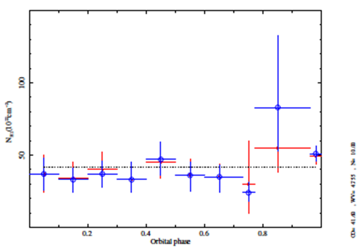
Fig. 21 Evolution of the absorption column N1H (ISM plus local absorption). Red filled squares: from equation (2). Blue open circles: from equation (5). The dotted line represents the fit to a constant. A better fit could be obtained by applying equation (10), but the large uncertainties prevent us from draw by firm conclusions. The color figure can be viewed online.
5. Summary and Conclusions
We have investigated the long-term variation of spectral parameters exploiting the continuous monitoring of Cen X-3 with MAXI/GSC and its outstanding spectral capabilities. From the analysis of the MAXI/GSC light curve, we estimated the orbital period of the binary system, Porb = 2.0870 ± 0.0005 days, which agrees with the value given by Nagase et al. (1992) and Rodes et al. (2017), and we also noticed the presence of a superorbital period of Psuperorb = 220 ± 5 days which is included in the interval [93.3-435.1] days reported by Sugimoto et al. (2014), who detected it by using a power spectrum density technique.
We have described the X-ray spectra of Cen X-3 by two models consisting of a blackbody plus a power law and a Comptonisation of cool photons on hot electrons plus a power law, both modified by an absorption covering fraction factor and Gaussian functions, and have performed detailed spectral analysis (orbital phase-averaged and phase-resolved, in the 2.0-20.0 keV range). Our results can be summarised as follows:
- The blackbody emitting area has an averaged radius of 0.71+0.19-0.16 km and its size varies from 1 or 3 km out-of-eclipse, which is consistent with a hot spot on the NS surface, to 9 ± 3 km in eclipse, covering a much larger area.
- From the unabsorbed flux, the total X-ray luminosities in the 2.0-20.0 keV were found to be (1.9+1.0-0.8) × 1037 erg s−1 (equation 2) and (2+3−1) × 1037 erg s−1 (equation 5) on average. This high luminosity in the long term, one order of magnitude larger than that for wind-fed X-ray binaries, indicates that accretion must be enhanced by other mechanisms. In the case of Cen X-3, this should be due to an accretion disc, matter co-rotating with the compact object and/or soft X-ray reflection from the inner accretion disc region. In addition, the out-ofeclipse X-ray luminosity was 10-30 times higher than in eclipse.
- From the comparison of the high-state, low-state and averaged spectra, it has been deduced that the emission region is compatible in size and consistent with thermal emission produced at the NS polar cap. The values obtained for the high and low state luminosities suggest that the difference can be attributed to a drop in the accretion rate rather than an overall enhancement of absorption.
- The column density of absorbing matter has two components: N2H ≈ (2 - 7) × 1022 cm−2 which represents the ISM towards the system and N1H ≈ (2 - 8) × 1023 cm−2, and both models yield similar column densities estimates within errors.
- The spectra show the iron fluorescence line at ≈ 6.4 keV which is detected by MAXI/GSC but it cannot resolve recombination iron lines. The description of the iron line complex adopted in this work suggests the presence of both near neutral iron line (Fe Kα) and highly ionised species (Fe XXV and Fe XXVI) except in the eclipse and egress spectra, where none of the emission lines are detected. No modulation along the orbit is seen in the line intensities.
- The orbital dependence of the column density was compatible with a constant value within errors. The large value of the column density N1H ≈ 4 × 1023cm−2 strongly favours a highly inhomogeneous surrounding environment. To better constrain the Cen X-3 stellar wind properties it is necessary to improve uncertainties of the parameters, especially the column density and EW of iron emission lines, for probing the geometry and distribution of circumstellar matter around the compact object. Numerical simulations performed by Blondin et al. (1991) were not able to well describe the observed behaviour for Cen X−3.

