


 nova página do texto(beta)
 Inglês (pdf)
 Artigo em XML
 Referências do artigo
 Enviar este artigo por email
 Citado por SciELO
  Similares em
SciELO
Similares em
SciELO 
 Permalink
1. INTRODUCTION
V563 Lyr (BD+40 3480, NSV 11321, NSVS 5499431, TYC 3122-495-1) was discovered by Hoffmeister (1965) as one of his many variables. It was later listed in the NSVS (Kukarkin & Kholopov 1982). There were 44 visual minimum estimates performed between 1995 to 1997 (Beltraminelli and Dalmazio 1999), and Beltraminelli et al. (1999) then obtained three new photoelectric minimum timings, thereby refining the period. The latter also obtained photoelectric observations in B and V; displayed the light curves in V and B-V, and concluded that the system was a contact binary belonging to the W UMa type. Based on the B-V colour index, they estimated the spectral type to be F5.
After that there were many eclipsing timings reported in the literature, and Akerlof et al. (2001) indicated that the system was part of the ROTSE survey (Akerlof et al. 2000).
V563 Lyr was included in the multi-paper DDO radial velocity studies (Pribulla et al. 2009). However, they noted difficulty owing to the system’s faintness (10.96 to 11.47 magnitudes in V) which resulted in “noisy spectra”. Further, they were able to obtain spectra at only the first quadrature (with a single exception); hence a spectroscopic mass ratio was not determinable. However, they did identify a third component in the spectra with velocity RV3 ≈ 14 km/s and ‘roughly’ estimated a mass ratio of 0.37. They also noted that the J-K index (0.216) was more indicative of a spectral type F2-3 and that the (anomalously higher) B-V index of 0.456 was likely due to interstellar extinction.
As there is no report of a Roche-based study involving both photometric and spectroscopic observation in the literature, this study was undertaken.
2. Period Variation
An eclipse timing difference (O−C) plot is reproduced in Figure 1. The reader will notice a large scatter in the timings from cycle -4000 (1997) to 4000 (2008) which is puzzling, as all the timings but one are either photoelectric (PE) or CCD. After 2008, the period appears to be constant, but at a higher value. A few of the data points with errors > 0.005 days have been removed at the request of the referee.
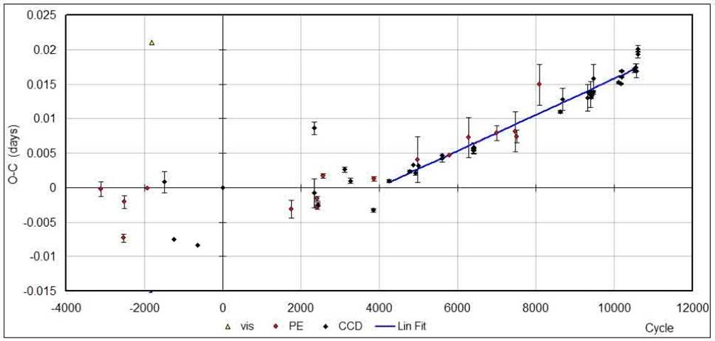
Fig. 1 The eclipse timing difference (O−C) plot for V563 Lyr. Open (yellow in the online version) triangle - visual; open (red) circle - photoelectric; black diamond - CCD. The elements used for phasing were [24 52500.2746, 0.5776412]. The data range is from 1997 to 2018. The colour figure can be viewed online.
The weighted least-squares best fit for the data after cycle 4000 yielded the following elements in equation 1, used for all phasing.
An Excel worksheet containing all available timing data is available online at Nelson (2019 and 2020a).
3. Spectroscopic Observations
This observer obtained in 2016, 2018, 2019, and 2020 a total of 20 medium-resolution (R ≈ 10 000) spectra at the Dominion Astrophysical Observatory (DAO) in Victoria, British Columbia, Canada using the 1.83-m Plaskett telescope. Windows software RaVeRe, written by the author and available at (Nelson 2013, Nelson 2020a), was used for reduction. The radial velocities (RVs) were determined by the broadening functions (BF) routine (Ruciński 1992, 2004; Nelson 2010) as implemented in the Windows-based software Broad (Nelson 2013, 2020a). See Nelson (2020b) for further details. The elements used for all the phasing are given in equation [EQ1] above.
A log of observations and the derived heliocentric radial velocities (RV1,2,3) is presented in Table 1.
Table 1 Log of DAO Observations and Results
| DAO Image # | Mid-Time (HJD-2400000) | Exposure (sec) | Phase at Mid-exp | RV1 (hel) (km/s) | RV2 (hel) (km/s) | RV3 (hel) (km/s) |
|---|---|---|---|---|---|---|
| 20-19141 | 59090.7 | 3000 | 0.159 | -127.0 (3.7) | 238.1 (3.6) | 6.1 (3.2) |
| 20-19449 | 59098.8 | 3000 | 0.162 | -107.4 (7.2) | 240.0 (5.1) | 16.7 (3.6) |
| 18-5459 | 58241 | 2750* | 0.170 | -97.7 (3.8) | 229.7 (3.6) | 27.9 (3.2) |
| 19-16500 | 58737.8 | 3000 | 0.181 | -111.0 (8.3) | 238.4 (8.1) | 17.0 (7.6) |
| 20-19574 | 59101.7 | 3000 | 0.182 | -118.0 (3.6) | 256.1 (3.2) | 13.8 (4.0) |
| 16-9400 | 57647.8 | 3600 | 0.218 | -131.3 (5.5) | 265.5 (4.1) | 11.6 (2.1) |
| 20-19396 | 59097.7 | 3000 | 0.274 | -113.5 (3.8) | 265.6 (8.9) | 17.7 (3.4) |
| 16-9347 | 57646.7 | 3600 | 0.288 | -129.1 (3.8) | 269.6 (3.9) | 11.9 (1.6) |
| 18-5305 | 58233 | 3000 | 0.309 | -130.2 (7.7) | 267.6 (2.4) | 8.1 (4.8) |
| 20-19583 | 59101.8 | 3000 | 0.342 | -97.6 (4.2) | 249.7 (5.7) | 24.2 (3.4) |
| 16-9365 | 57646.9 | 3600 | 0.647 | 159.1 (3.9) | -181.7 (3.3) | 23.6 (4.8) |
| 18-5384 | 58234.9 | 3000 | 0.651 | 144.0 (3.3) | -190.8 (4.0) | 15.1 (3.8) |
| 18-5489 | 58241.9 | 1798* | 0.704 | 150.0 (2.3) | -216.1 (3.3) | 17.6 (3.6) |
| 16-9299 | 57645.8 | 3600 | 0.717 | 155.1 (3.1) | -212.7 (5.1) | 21.8 (3.5) |
| 16-9473 | 57652.7 | 3600 | 0.728 | 169.6 (6.1) | -220.0 (4.2) | 29.6 (5.2) |
| 20-19485 | 59099.7 | 3000 | 0.742 | 159.3 (6.5) | -217.5 (7.3) | 25.8 (4.4) |
| 18-5495 | 58241.9 | 3000 | 0.799 | 156.1 (4.8) | -206.9 (3.4) | 22.3 (5.4) |
| 20-19487 | 59099.7 | 3000 | 0.803 | 164.4 (7.3) | -199.4 (3.1) | 27.6 (4.4) |
| 20-19050 | 59088.8 | 3000 | 0.810 | 147.5 (6.7) | -192.7 (2.0) | 22.7 (4.0) |
| 19-16544 | 58745.6 | 2400 | 0.815 | 147.6 (9.0) | -192.5 (9.4) | 14.6 (9.1) |
*Clouds caused the exposure to be terminated early.
The calibrated one-dimensional spectra, sorted by phase, are presented in Figure 2.
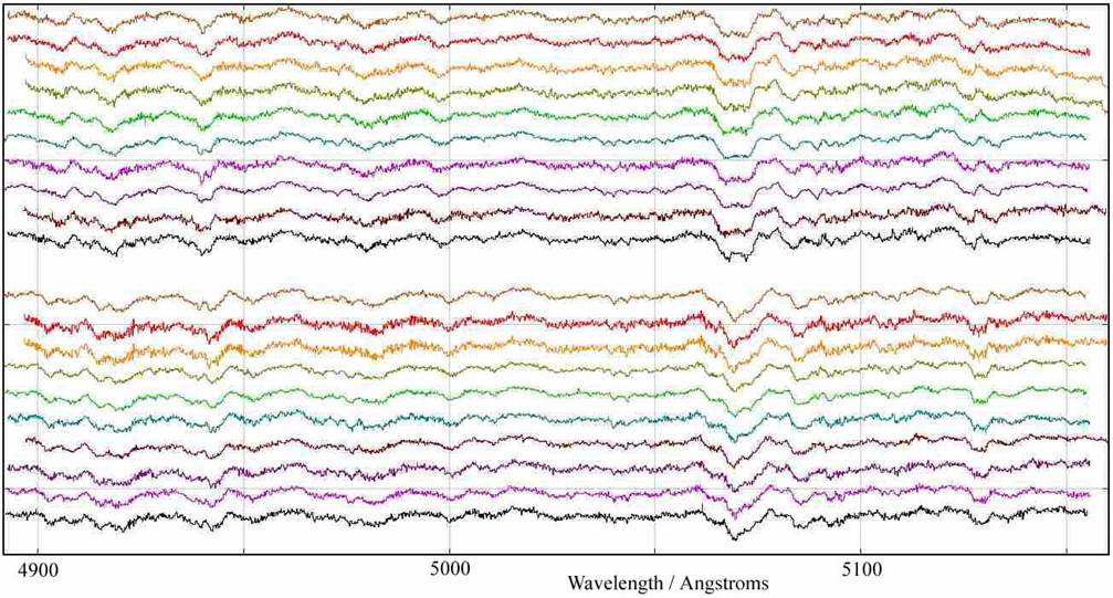
Fig. 2 V563 Lyr spectra, offset for clarity. The vertical scale is arbitrary. The phases (from top to bottom) correspond to those in Table 1, top to bottom. The colour figure can be viewed online.
As noted above, RV determination was by the broadening function method due to Rucinski. In most previous light curve modelling papers by this author (for example, Nelson 2017, Nelson 2020b), broadening functions were also used, and radial velocities extracted by smoothing the broadening function to remove noise, then centroiding the peaks that ensued. In the case of V563 Lyr, smoothing the peaks and centroiding is not appropriate owing to the likely presence of a third star, whose peak is obvious in the broadening functions, and which would contaminate the broadening functions from the other stars.
To disentangle the components, Gaussian profile curve fitting was developed in Excel (and later added to software Broad). The Gaussian profile for each of the three stars required three parameters: central velocity v 0, amplitude A, and ‘width’ w (the actual full width at half maximum of the Gaussian profile being 2 · w · ln{21/2}). The modified form of the standard Gaussian function is given in equation 2 (where i denotes the star index number i = 1-3).
The sum of the three functions was then taken as the theoretical curve, labelled in Figures 3-5 as ‘sum’, and the observed BF values, displayed as dots. The individual Gaussian components are also displayed. The sum of the differences squared (between the observed and theoretical values) was then optimized by adjusting the nine parameters. In Excel, the ‘Solver’ facility (which uses the Generalized Reduced Gradient code) was used, whereas software Broad uses the Levenberg-Marquardt (L-M) algorithm. (The former method is quite stable and almost always finds a solution, but may not be a relevant one, depending on the initial parameters, whereas the second requires a more critical choice to avoid crashes.). To avoid nonsensical results, care was taken to cut off computation at certain lower and upper velocities. These cutoff values were usually set manually at the points where the observed BFs would first cross the x-axis (or nearly so) upon descent from the central peaks. (For example, in Figure 3, the lower limit was -220 and the upper, +260 km/s.). The results were found to be very insensitive to the choice of cutoff values, and any differences that resulted (typically 1 or 2 km/s) were well within error limits.
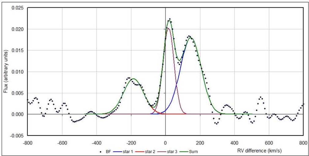
Fig. 3 Broadening function for V563 Lyr at phase 0.654 and the fitted Gaussian profiles. The standard spectrum is 18-5223 (HD 126053) and the program spectrum, 18-5384. The colour figure can be viewed online.
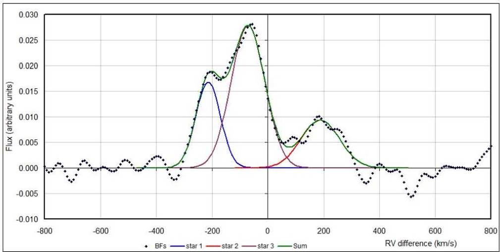
Fig. 4 Broadening function for V563 Lyr at phase 0.311 and the fitted Gaussian profiles. The standard spectrum is 18-5178 (HD 114762) and the program spectrum, 18-5305. (This corresponds to the third data line in Table 2). The colour figure can be viewed online.
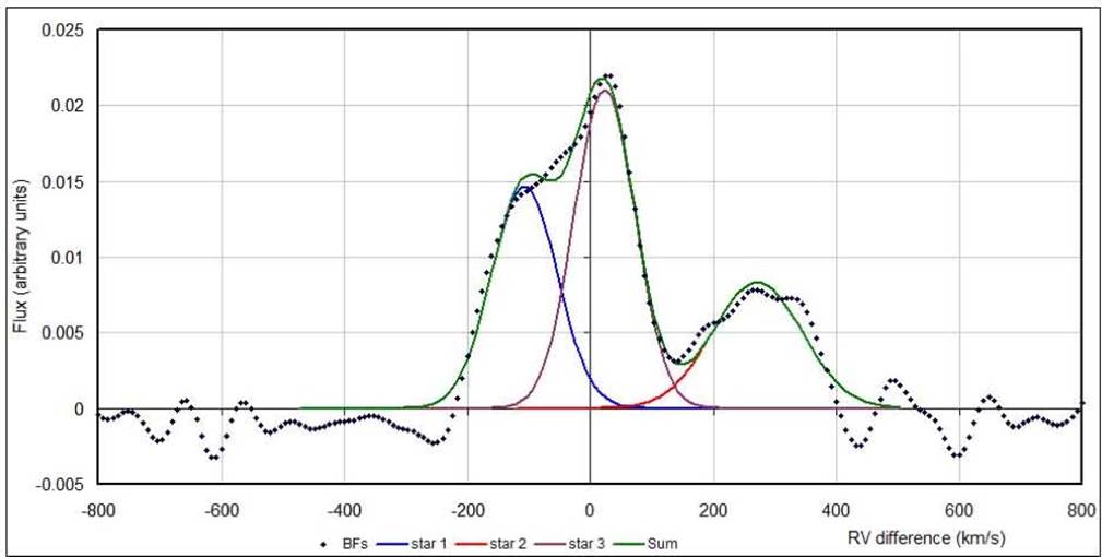
Fig. 5 Broadening function for V563 Lyr at phase 0.311 and the fitted Gaussian profiles. The standard spectrum is 18-5258 (HD 187691) and the program spectrum, 18-5305. (This corresponds to the sixth data line in Table 2). The colour figure can be viewed online.
Note that, in Figure 3, the BF for the particular combination of comparison and program spectra, at phase 0.654, shows a clear separation of peaks. Note also the slight ‘peak pulling’ on the profile for Star 1 (on the right) due to the presence of the third star. Had the peak centroiding method been used, a distorted value for RV1 would have ensued.
In view of the relatively long exposures relative to the period, a phase smearing correction was applied in each case. For details of, and a mathematical justification for, this procedure, the reader should consult Alton et al. (2020).
Figures 4 and 5 display the situation for the previous night when the opposite phases were experienced. Both are for the same program spectrum but use two different comparison spectra. For Figure 4, peak centroiding could again have been used, but again with peak pulling for Star 1.
In Figure 5 a different comparison spectrum was used but this time there is no definite peak for Star 1. One might wonder about the validity of the profiling method in this case. To compare results, we present in Table 2 the data for the one target spectrum and all seven different comparisons for that reduction.
Table 2 The BF Profile-Fitting Results for Program Spectrum 18-5305*
| Std File# | RV std name | RV1 (Hel) km/s | RV2 (Hel) km/s | RV3 (Hel) km/s |
|---|---|---|---|---|
| 18-5167 | HD 089449 | -125.2 | 263.6 | 9.9 |
| 18-5172 | HD 102870 | -130.6 | 263.9 | 10.2 |
| 18-5178 | HD 114762 | -141.8 | 263.4 | 9.2 |
| 18-5184 | HD 140913 | -121.4 | 261.3 | 14.3 |
| 18-5233 | HD 126053 | -122.3 | 260.1 | 12.2 |
| 18-5258 | HD 187691 | -119.1 | 259.0 | 13.6 |
| 18-5261 | HD 154417 | -129.7 | 257.9 | 8.6 |
*Converted to heliocentric RVs. The last column con- tains the RVs for the putative companion star. (See later discussion).
The means and standard deviations for RV1, RV2, and RV3 in this table are -127.2 (7.7), 261.3 (2.4), 11.1 (2.2) km/s, respectively. Note the very small scatter in RV2 and RV3. The scatter in RV1 is, in the experience of this observer, not excessive, but clearly the proximity of the stronger and sharper BF due to Star 3 complicates matters.
The reader will also note that, between Figure 4 and 5, the widths of the Gaussian functions for RV3 are significantly different. This is somewhat troubling, as the heights and widths of the broadening peaks should reflect some physical values. The differences are likely due to the same errors in the Gaussian fitting approach-which rightly ought to be investigated thoroughly-but which would be better suited to a separate paper. In any case, the results seem reasonable.
Our mean value for RV3 (for this target spectrum) is virtually consistent with the value (, no error estimate) provided by Pribulla et al. (2009).
In § 5, we will need the ratio of the flux from Star 3 compared to the total flux (at phases 0.25 and 0.75). As the BF process is linear (Rucinski, undated private communication), we may obtain an estimate of the flux from a given component by taking the area under its Gaussian profile, which is proportional to amplitude Ai times width wi as defined in equation 2; thus we have flux Fi = k · Ai · wi where k is a constant that drops out when ratios are taken. The fraction of the flux contributed by the third star is then F3 / (F1 + F2 + F3) = 0.29 (7) in this case, averaged over the entire dataset (the figure in brackets is the standard deviation in units of the last digit). This value will be compared with the results from the photometric analysis which, of necessity, involves third light. The relevant photometric passband would be V, as it most closely approximates the wavelength range over which the spectra were taken.
The derived (heliocentric) RV values are listed in Table 1 along with the error estimate for each, the latter being the standard deviation of values from the different comparisons as presented above. The overall (i.e., through all phases) heliocentric radial velocity of the third star was RV3 = 18.8 ± 6.7 km/s. This is compatible with the centre of mass RVγ of the eclipsing pair (see later discussion).
4. Photometric Observations
Photometric observations were carried out at Desert Blooms Observatory in 2019 (April-May). Obtained were a total of 742, 743, and 744 observations in B, V, and Ic respectively. The telescope is a 40 cm Schmidt-Cassegrain optical assembly operating at f/6.8; data acquisition was by a QSI 683 CCD camera (see Nelson 2020b for more details).
In Table 3, the coordinates for the stars of interest are presented, taken from the Tycho-2 Catalogue (Høg et al. 2000). The magnitudes are taken from the AAVSO Photometric All-Sky Survey (APASS, DR9; Henden et al. 2009). The colour index of the comparison was higher than one would like; however, most of the possible candidates in the field had similar values. The star chosen for the comparison had the advantage of close proximity and being close in brightness to the program star. (But see § 7 for a further discussion of comparison selection.) For all the runs, the difference C - K was observed to be constant to within ≈ 0.01 magnitude, with no systematic variation.
Table 3 The Variable, Comparison and Check Stars for V563 Lyr Photometric Observations
| Object | TYC/GSC | RA (J2000) | Dec (J2000) | Spec. | V (mag)* | B-V) (mag)* |
|---|---|---|---|---|---|---|
| Variable | 3122-495-1 | 18:45:06.6 | +40:11:11.5 | F5 | 11.112 (20) | 0.282 (20) |
| Comparison | 3122-1487 | 18:44:53.5 | +40:10:03.5 | - | 11.944 (20) | 1.147 (20) |
| Check | 3122-2865 | 18:45:16.7 | +40:12:26.9 | - | 12.128 (20) | 0.749 (20) |
*The APASS catalogue provided no error estimates, so 0.020 mag was assumed (in view of the faintness of the stars).
As described in Nelson (2020b), automatic focusing was required to accommodate the large swings in temperature throughout each night.
The usual bias and dark subtraction, and flat fielding, as well as aperture photometry was accomplished with MIRA (by Mirametrics).
5. Light Curve Analysis
Curve fitting was undertaken with the 2003 version of the Wilson-Devinney (WD) light curve and radial velocity analysis program with the Kurucz atmospheres (Wilson and Devinney 1971, Wilson 1990, Kurucz 1993, Kallrath et al. 1998, Kallrath & Milone 2009) as implemented in the Windows front-end software WDwint56c (Nelson 2013). RV and light curve data from the this paper were used in a simultaneous fit.
As mentioned above, the classification of Beltraminelli et al. (1999) was F5. Also, the 2MASS catalogue (Skrutskie et al. 2006) yielded values J = 10.286 (26) and H = 10.120 (31) so then J - H = 0.166. Reference to interpolated tables from Cox (2000) as augmented with infrared data from Mihalas and Binney (1981) confirmed the designation. The tables of Pecaut and Mamajek (2013) yielded a temperature T = 6510 (120) K, and a log g = 4.355 (8) (cgs) where the errors correspond to the differences over one spectral subclass. An interpolation program by Terrell (1994, available from Nelson 2013) gave the Van Hamme (1993) limb darkening values; and finally, a logarithmic (LD=2) law for the limb darkening coefficients was selected, appropriate for temperatures > 8500 K (ibid). The limb darkening coefficients are listed below in Table 4. Values for the gravity darkening exponent g = 0.32 and albedo A = 0.5 were chosen, appropriate for convective stars (Lucy 1967 and Ruciński 1969, respectively).
Table 4 Limb Darkening Values from Van Hamme (1993) Based on Spectral Type F5, F5-6 For Stars 1 and 2 Respectively*
| Solution 1 | Solution 2 | |||||||
|---|---|---|---|---|---|---|---|---|
| Band | x1 | x2 | y1 | y2 | x1 | x2 | y1 | y2 |
| B | 0.806 | 0.813 | 0.233 | 0.213 | 0.835 | 0.841 | 0.153 | 0.129 |
| V | 0.710 | 0.723 | 0.275 | 0.269 | 0.756 | 0.767 | 0.240 | 0.223 |
| Ic | 0.553 | 0.567 | 0.276 | 0.271 | 0.601 | 0.612 | 0.254 | 0.242 |
| Bol | 0.639 | 0.640 | 0.241 | 0.234 | 0.646 | 0.648 | 0.214 | 0.203 |
*The same coefficients are listed for Solution 2 (discussed later) where the estimated spectral types are G1 and G4.
Based on the shape of the light curve, Mode 3 (overcontact binary) was selected. Initially, convergence by the method of multiple subsets was reached in a relatively small number of iterations. The subsets were: (a, Ω1, L1), (i, T2, q), (T2, Ω1), (T2, q), and (a, Vgam, φ). In view of the fact that a companion was known to be present (from the spectra), it was appropriate to add third light (and also necessary to reach a solution). Therefore EL3 was a parameter, as was also a spot, added to Star 1. However, the correct choice of EL3 proved to be elusive, as the fit (as indicated by the sum of residuals squared) proved to be a weak function of the EL3 values selected, and differential corrections was unable to provide meaningful corrections. To overcome this problem, for each band, a value for EL3 was selected and the fit optimized by altering the other parameters (especially T2, q, and inclination i). Next, a new value for EL3 was chosen and the fit optimized again. In this way, the optimum value of EL3 for that band was determined. The procedure was then applied to the remaining bands.
In the original solutions there was a problem (picked up the referee) in that the values of EL3 were inconsistent with the ratio of fluxes derived from the broadening functions (see § 3), being an order of magnitude too low. This was despite the fact that the solution minimized the residuals and appeared to give a good fit visually. Thereafter, higher values of flux quantity EL3, starting with ≈ 0.2 for each band, were used in renewed modelling, and a grid search was followed, as above, to find a solution. The final values were EL3 = 0.257 (3), 0.256 (3), 0.245 (3) for B, V, Ic respectively. In determining the luminosity L3 of star 3, one needs to assume that it radiates isotropically. If that assumption is made, we may take L3 = 4 π EL3 (Wilson and van Hamme 2013). The values for third light (luminosity) ratio L3/(L1 + L2 + L 3) are listed in Table 5 and repeated in Table 7 along with those for the other components.
Converting the EL3 (B) and EL3 (V) flux values to magnitudes and carrying through the errors rigourously, we have B - V = 0.004 ± 0.036 mags. With the estimated B - V colour index of the third star at hand we have, using the tables of Pecaut and Mamajek (2013) we estimate the spectral type of Star 3 as A0 ± 1 spectral subclass. Note that the above derivation neglects interstellar absorption.
The above solution so achieved is presented in Table 5 as Solution 1.
Table 5 Wilson-Devinney Parameters for the Best-Fit Solution for V563 Lyr. Solution 2 is to be Preferred (See Discussion)
| WD Quantity | Sol’n 1 | Sol’n 2 | WD Quantity | Sol’n 1 | Sol’n 2 |
|---|---|---|---|---|---|
| Temperature T1 (K) | 6510* | 5837* | L1/(L1+L2) (B) | 0.634 (4) | 0.646 (4) |
| Temperature T2 (K) | 6385 (7) | 5689 (3) | L1/(L1+L2) (V) | 0.628 (4) | 0.637 (4) |
| q = m2/m1 | 0.583 (14) | 0.563 (28) | L1/(L1+L2) (Ic) | 0.622 (3) | 0.629 (3) |
| Potential ω1 = ω2 | 2.797 (71) | 2.797 (155) | L3/(L1+L2+L3) (B) | 0.276 (3) | 0.276 (3) |
| Inclination i (degrees) | 79.2 (2) | 78.2 (1.1) | L3/(L1+L2+L 3) (V) | 0.271 (3) | 0.271 (3) |
| Semi-maj. axis, a (R⊙) | 4.61 (5) | 4.61 (6) | L3/(L1+L2+L3) (Ic) | 0.259 (2) | 0.259 (2) |
| Centre of mass RVγ (km/s) | 26.6 (1.8) | 26.6 (9) | r1 (pole) (orbital radii) | 0.442 (14) | 0.442 (14) |
| Fill-out factor f1 | 0.685 (32) | 0.685 (32) | r1 (side) (orbital radii) | 0.478 (20) | 0.478 (20) |
| Spot co-latitude (deg) | 38 (2) | 36 (2) | r1 (back) (orbital radii) | 0.531 (31) | 0.531 (32) |
| Spot longitude (deg) | 173 (1) | 173 (1) | r2 (pole) (orbital radii) | 0.354 (15) | 0.354 (16) |
| Spot radius (deg) | 20.5 (2) | 20.7 (5) | r2 (side) (orbital radii) | 0.378 (20) | 0.378 (20) |
| Spot temp. factor | 0.852 (1) | 0.846 (1) | r2 (back) (orbital radii) | 0.454 (49) | 0.454 (50) |
| Σω2res | 0.23058 | 0.24186 | - | - | - |
*Held fixed.
Pribulla et al. (2009) estimated the luminosity ratio L 3/(L1+L2) = 0.15 (presumably in the V band). Taking the value in Table 5 of L3/(L1+L2+L3) (V) = 0.271 (3) and using simple algebra we have L3 / (L1 + L2) = 0.371 (4). The cause of the discrepancy between the two corre- sponding values is not clear.
The light curves, computed light curves and the residuals in the sense data-computed are plotted in Figure 6.
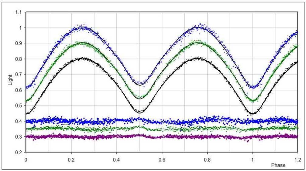
Fig. 6 V563 Lyr light curves and the WD results, separated by fixed offsets (0.1 light curve units). Plotted are, top to bottom: B, V, Ic. At the bottom of the figure, the differences in the sense observed-calculated; the order is the same as for the light curves. The colour figure can be viewed online.
Next, the radial velocity data and solutions are plotted, starting with the RVs from this paper, in Figure 7. A simple double-sine fit yields values K1 = 147.4 (2.1) km/s and K2 = 247.1 (1.1) km/s, and RVγ = 22.5 (1.5) km/s). The spectroscopic mass ratio is qsp = M2/M1 = K1/K2 = 0.596 (8). Note that the mass ratio in Table 5 derived from combined (RV + LC) fitting differs somewhat from the spectroscopic mass ratio calculated from the ratios K1/K2. This is normal; however, the former is considered more reliable as it is derived from all the data (Wilson 1990). In any case, the error bars virtually overlap.
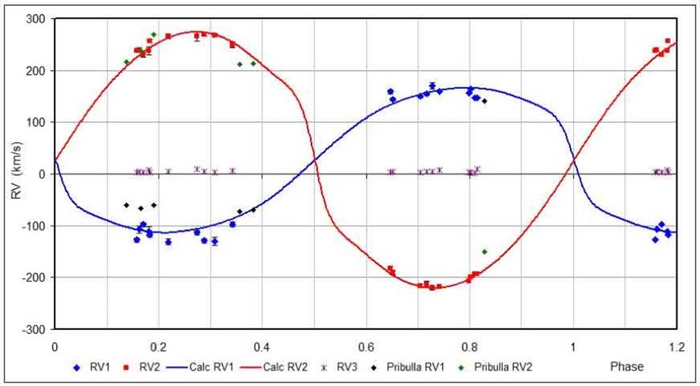
Fig. 7 V563 Lyr radial velocities and WD solution. The radial velocities of the third star appear near the x-axis. The RV1 and RV2 values from Pribulla et al. (2009) appear as the (black) and (green) diamonds, resp. From [ibid] there is a single point in the second half of the cycle. The colour figure can be viewed online.
A word about error estimation is appropriate here (all error values in this paper are one sigma). For the errors in K1 and K2, the reader should consult Alton et al. (2020). For the individual RV data points in the present dataset, each RV is the mean of values obtained from eight different standards; the error estimate is simply the standard deviation of the group. Actual errors from systematic effects are obviously larger but not directly calculable. That is why the sample standard deviation (i.e., sigma divided by root n) is not used, as it would imply a greater precision than what is experienced.
The visual representation of Binary Maker 3 (Bradstreet 1993) is presented in Figure 8.
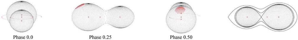
Fig. 8 V563 Lyr three-dimensional representation from Binary Maker 3, at the phases indicated, and the surface potentials. The colour figure can be viewed online.
The WD output fundamental parameters and errors are listed in Table 6. Most of the errors are output or derived estimates from the WD routines. These are statistical errors and known to be smaller than total errors because the latter contain systematic errors not readily available.
Table 6 V563 Lyr Fundamental Parameters. Solution 2 is to be Preferred (See Later Discussion)
| Solution 1 | Solution 2 | |||
|---|---|---|---|---|
| Quantity | Star 1 | Star 2 | Star 1 | Star 2 |
| Spectral type | F5 | F5-6 | G1 | G4 |
| Temperature, T (K) | 6510* | 6385 (7) | 5837* | 5689 (3) |
| Mass, (M /M⊙) | 2.49 (4) | 1.45 (4) | 2.49 (4) | 1.45 (4) |
| Radius, R (R⊙) | 2.23 (2) | 1.81 (2) | 2.23 (2) | 1.81 (2) |
| M bol (mags) | 2.52 (3) | 3.06 (3) | 3.00 (3) | 3.56 (3) |
| Log g (cgs units) | 4.14 (1) | 4.08 (1) | 4.14 (1) | 4.08 (1) |
| Luminosity, L (L/L⊙) | 7.73 (68) | 4.70 (41) | 4.97 (44) | 2.96 (26) |
In the last few light curve modelling papers by this author, it has been the norm to use differential photometry, the Gaia distance (Luri et al 2018), the interstellar absorption Av, and the bolometric corrections (BCs) to estimate the luminosities. This independent calculation of the latter serves as a check on the spectral type and hence the effective temperature of the more luminous component. We shall do so now. The calculation proceeds as follows:
Differential photometry at phases 0.23-0.27 and 0.73-0.77 (when both stars were visible broad-side) yielded the following instrumental differential magnitudes: ∆b = bvar − bcomp = −1.800 ± 0.001 mag and ∆v = vvar − vcomp = −0.995±0.006 magnitudes.
The standard formulae for transformation from instrumental to Johnson magnitudes are given in equations 3 and 4 (Henden and Kaitchuk 1982):
where ε = - 0.032 ± 0.001 and µ = 1.086 ± 0.010 are the transformation coefficients for the camera + filter setup at DBO (Alton 2017). Operating differen- tially, the trailing constant ς drops out, and substi- tuting equation 4 into 3 (and simplifying some sub- scripts) we have equation 5:
where Vc = 11.944 ± 0.020 mags given in Table 3. Combining terms (with the errors added in quadrature) one obtains V = 10.977 ± 0.012 mags.
Next, the presence of third light must be addressed. According to Wilson and van Hamme (2013), if one assumes that the third star emits light isotropically, one may write equation 6:
where l3 is the same as EL3 used in the WD code and used above. Note that Wilson and van Hamme point out that simply listing EL3, as what one might want to do, is meaningless unless one also specifies the L1 and L2 values. As a result, we list L3 /(L1 + L2 + L3) in Table 7.
Table 7 Relative Luminosities of the Three Components (Assuming a Third Star, and If so, that the Latter Emits Isotropically)
| Band | L1 / (L1+L2 + L3) | L2 / (L1 + L 2+L3) | L3 / (L1+L 2+L3) |
|---|---|---|---|
| Blue, B | 0.459 (3) | 0.265 (1) | 0.276 (3) |
| Visual, V | 0.458 (2) | 0.272 (1) | 0.271 (3) |
| Infrared, Ic | 0.461 (2) | 0.280 (1) | 0.259 (2) |
Using the computed luminosity ratios L1 / (L1+L2+L3) and L2 / (L1+L2+L3) for the V band, one finds the individual magnitudes V1 = 11.825 (21), and V2 = 12.392 (21) by using equation 7.
where i = 1, 2. Determination of the interstellar extinction was from the formulations of Amôres and Lepine (2005), and depending on the model, one obtains values of Av = 0.275, 0.248, and 0.124 mags with a mean value of 0.216 (71) mags, where the error is the sample standard deviation of the three values.
Then, using the standard formula (equation 8) applied to each star we have equation 8:
whence the individual values for each star are Mbol,1 = 2.994(31) mags and Mbol,2 = 3.556 (37). Converted to luminosities using the standard formula and making use of the bolometric magnitude of the Sun as Mbol,Sun = 4.74 mags (Cox 2000) we have the photometric luminosities L1 = 5.0 (1.3) L⊙ and L2 = 3.0 (9) L⊙ where the largest error source is from the Gaia distance. These values, are significantly lower than the WD output in Table 6.
Despite the rather large errors in the photometric luminosities, it seemed important to adjust the effective temperature T1. This is especially true because the spectral classification of Beltraminelli et al. (1999) was based on the colour index (B - V) and, as we have seen, the flux received is contaminated by the significant contribution of the hot third star (spectral type ≈A0). Making use of the well-known black body law of equation 9
we may write equation 10
This is significantly lower than the original value and places the spectral type for Star 1 at ≈ G1. Continuing on, and using this lower value for T1, a revised solution was derived in a relatively few steps. The final value for T2 was 5689 K which would place the spectral type as ≈ G4. The results are listed in Tables 5 and 6 as Solution 2.
6. Evolutionary Status
It is possible to investigate the evolutionary status of this system with the aid of data from Yakut and Eggleton (2005), who collected data for some 72 close binary systems for which reliable data existed. Types included were low-temperature overcontact binaries, near-contact binaries and detached close binaries. Figure 9 reproduces their plot of log L vs Log T, with the zero-age main sequence (ZAMS) values for isolated stars from Cox (2000), and the terminal-age main sequence (TAMS) values from the evolutionary tracks of the Geneva Group (Schaller et al. 1992) for Z = 0.02 (solar).
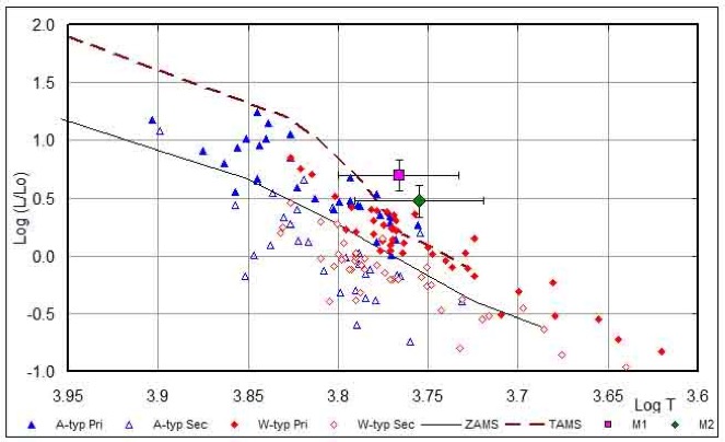
Fig. 9 Log L vs Log T plot for EW-type binaries from Yakut and Eggleton (2005). The ZAMS (solid line) and the TAMS are from the evolutionary tracks of the Geneva Group (Schaller et al. 1992) for Z = 0.02 (solar). The results from Solution 2 have been added: the large square (pink in the online version) is for Star 1 while the large (green) diamond is for Star 2. The (half) width of each error bar is the standard deviation of the values for log T1,2 and log L1,2 from each solution. The colour figure can be viewed online.
This plot suggests both stars have evolved and might be past the TAMS. As a referee from a previous paper has noted, one should regard plots of this type with much caution, as we do not know the metallicity, and in any case there is a fairly large degree of uncertainty with the temperatures and luminosities for this system. The error bars hint at that uncertainty. What is needed is an analysis of a classification spectrum that would decompose the component spectra.
7. Discussion
Further to the use of Gaussian profile fitting for extracting RVs from the broadening functions (rather than smoothing and peak centroiding), it has been found that, even for the detached peaks noted in Nelson (202b), profile fitting gives more consistent results, and is now used on a regular basis by this observer for all RV determinations.
The matter of choice of the comparison star selection bears discussion. In light curve analyses, one rarely has the ideal comparison star which would be: (a) close in brightness, (b) close in spectral type, and (c) in close proximity in the image frame. If condition (a) is not followed and the stars are, say, more than a magnitude different in brightness, excessive shot noise will result because one of the stars will be underexposed. If condition (c) is not followed, less than ideal sky conditions may result in significant systematic deviations from the unaffected light curve from time to time, owing to significant variations in sky transparency over the sky area covered by the chip. For this observer, condition (b) is the one most readily relaxed. In answer to concerns by the referee of a previous paper regarding the choice of spectral type-matching of the comparison star, tests were rerun with a different comparison considerably closer in colour; there were no significant differences in the final parameters resulting from Wilson-Devinney modelling. Hence-within the limits of this test-the spectral-type matching of the comparison star would appear to be a non-issue.
Initial modelling runs of this system, as is so often the case for many overcontact systems, led to an early solution. However, the presence of spots and third light complicated matters (especially the latter), requiring many runs to achieve a convincing solution. Modelling with a bright spot at the back of Star 2 was attempted but gave poor results. The ready adoption of a solution that seemed to represent a minimum but for which there was an inconsistency between the strength of the third star BF and the weakness in the early adopted third star fluxes EL3 (for the phases 0.25 and 0.75) was problematic. Clearly the first solution was a local minimum; The takeaway from this is that modellers need to be aware that local minima exist and may not be represent consistency between all the observables. The lowest sum of residuals squared is not the only criterion.
The solution to the EL3 inconsistency was to start with some more realistic values (EL3 = 0.2) and do a grid search to find the optimum values; this was done and reasonable agreement between RV and photometric results was achieved. As noted above, the mean radial velocity (through all orbital phases of the eclipsing pair) of the putative third star (RV3 = 18.8 ± 6.7 km/s) and that of the centre of mass for the eclipsing pair (RVγ = 22.5 ± 1.5 km/s) are mutually consistent. At first glance, one might think that the third star would be in a mutual orbit with the eclipsing pair at inferior or superior conjunction, and therefore physically connected. How- ever, based on the relative luminosities, it is likely a fairly early spectral type, estimated as A0 ± 1 spectral subclass. Therefore its flux (were it at the same distance as the eclipsing pair, and a main-sequence type) would dominate that of the other two (G1 and G4). This was not observed. Therefore (Milone 2022) we are forced to the conclusion that the star is at a greater distance and therefore an accidental double. A high S/N classification spectrum at medium resolution might permit a disentangling of the spectral components which would settle the matter.
8. Conclusion
New radial velocity and photometric data for the overcontact binary V563 Lyr have been obtained and analysed with the 2003 version of the Wilson-Devinney code. Analysis of the radial velocity curves by fitting double sinusoidal curves yields values K1 = 147.4 ± 2.1 km/s, K2 = 247.2 ± 1.1 km/s, RVγ = 22.5 ± 1.5 km/s, and qsp = 0.596 ± 0.008. A third component has been identified, with radial velocity RV3 = 18.8 6.7 km/s which is in agreement with the findings of Pribulla et al. (2009) who found RV3 ≈ 14 km/s for the companion. Assuming an effective spectral type of F5, the following values for the masses, radii and luminosities of the eclipsing pair were obtained: M1 = 2.49(4) M⊙, M2 = 1.45(4) M⊙, R1 = 2.23(2) R⊙, R2 = 1.81(2) R⊙, L1 = 7.7(7) L⊙, and L2 = 4.7(4) L⊙. This has been labelled in Tables 5 and 6 as Solution 1.
However, a direct calculation of luminosities using photometry, the Gaia DR3 distance, the bolometric corrections, and estimated values for the interstellar extinction resulted in much lower luminosity values which were inconsistent with the values stated above (computed from WD modelling). As estimates of the spectral type of the companion were ≈ A0 and the fact that its contribution to the overall flux were comparable to that of Star 2, that would imply that the spectral types of the eclipsing pair were much later than the F5 value of Beltraminelli et al. (1999) - that is, to make the average spectral type appear to be F5. An estimate of the corrected value for T1 (based on the black body law) was 5837 ± 333 K, which would correspond to a spectral type of G1. Revised modelling with this lower T1 value resulted in the revised luminosities of the eclipsing pair: L1 = 5.0 (4)L⊙, and L2 = 3.0 (3)L⊙.
Inserting the derived parameters of the eclipsing pair into a log (L) - log (T eff) plot for each star using data from Yakut and Eggleton (2005) suggests that both stars are over-luminous and evolved to, and perhaps past, the terminal age main sequence.
The companion (Star 3) is estimated to have a spectral type A0 ± 1 spectral subclass. If it were gravitationally bound, the flux from a main sequence A0 type would dominate the light curves and broadening functions, so that cannot be. Simple computations reveal that a white dwarf (WD) would contribute only a very small flux-too small for what was observed. In any case, the broadening functions from a WD would be much wider than what was observed (Milone 2022). Possibly, the companion could represent an optical double, and therefore be at any distance (Milone 2022).
A high S/N classification spectrum at medium resolution might permit a de-convolution of the spectral components which would settle the matter as to its nature.

