


 nueva página del texto (beta)
 Inglés (pdf)
 Artículo en XML
 Referencias del artículo
 Enviar artículo por email
 Citado por SciELO
  Similares en
SciELO
Similares en
SciELO 
 Permalink
1. Introduction
Precise determination of stellar radial velocities is always affected by the superposition of convective blue- and redshifts in the upper stellar photosphere. Several authors (Dravins et al. 1981; Dravins 1990; Gray 2009) have addressed this issue, suggesting a method which, in principle, makes it possible to separate the contributions from convective velocities and the overall motion of the star. The key parameter is line depth: shallow or weak absorption lines originate in deeper layers where convective upwelling is fast, being more blueshifted than stronger lines which come from near the surface, where buoyancy disappears and gravity decelerates the convection. The result is a diagonal distribution of the line cores, which for the sun is quite narrow (Gray & Oostra 2018) with a velocity scatter between 50 and 100 m/s. If the granulation diagram of a star features a similar narrow diagonal, the standard solar curve, or a theoretical model curve (Ramírez et al. 2010), may be superposed on it, giving a trustworthy value for the stellar velocity and, as a bonus, an estimate of the strength of convection currents in the star.
Typically, such diagrams have a velocity scatter of about 200 m/s (Allende Prieto et al. 2002; Ramírez et al. 2010) which is shown by these authors to be of the same order of magnitude as the calibration plus reduction errors.
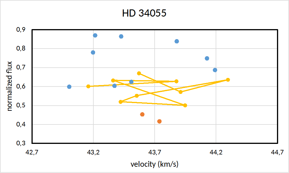
In cool giants, however, this explanation may not be sufficient, as can be seen, for example, in Gray & Pugh (2012). Sometimes the granulation diagrams show a broad distribution of line cores, with no consistent shape or slope (like the star HD34055 in Figure 6).
Besides measurement errors, several causes have been hinted at, correlating with line strength, excitation potential and wavelength region (Dravins et al. 1981). Here we explore another reason: observed wavelength shift may depend on the chemical species. This effect can be seen in Gray & Pugh (2012). We show that, in some stars, Ti I lines are systematically redshifted with respect to Fe I lines, and discuss the probable reason.
2. Data
2.1 Data Sources
We use spectra acquired with the UVES spectrograph (Dekker et al. 2000) and published under the Paranal Observatory Project POP (Bagnulo et al. 2003); this library offers a large sample of stellar spectra, distributed over a major part of the HR diagram, each covering the visible and near infrared at a resolution of 8 x 10⁴ and a sampling frequency of 49 data points per Å in our chosen wavelength range from 7400 Å to 7500 Å. For comparison with higher resolution data, we also use the Hinkle & Wallace spectral atlas of Arcturus (Hinkle et al. 2000), which features a resolution of 150000 and a sampling rate of 112 pixels per Å.
For line identification and rest wavelengths we use the VALD-3 database (Ryabchikova et al. 2015) from which we also extracted synthetic line depths for several stellar recipes.
2.2 Selection of Stars
The stars were selected from the Paranal Observatory Project (POP) database seeking to cover uniformly several photometric groups. As this source offers only the observed V magnitude, we checked SIMBAD (Wenger, M. et al. 2000) for parallax and multiband magnitudes, to locate the stars on the HR diagram (Figure 1). Three parallaxes reported in SIMBAD are from the revised Hipparcos data (Van Leeuwen 2007); the other ten are from Gaia EDR3 (Vallenari et al. 2021). We divided our sample into several groups according to the location on the HR diagram without any allusion to evolutionary status; in particular, the stars labeled “Red Clump” are not necessarily helium-burning stars.
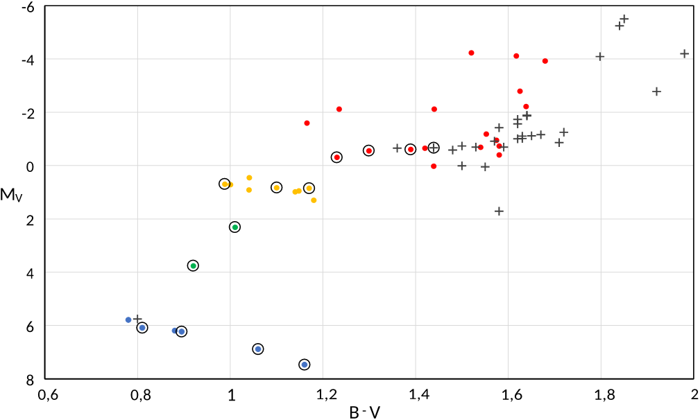
Fig.1. Shown are all K stars (dots) and M stars (crosses) included in the POP survey. The stars used in the present work are circled. We classify the K stars according to their location. Blue: main sequence. Green: subgiants. Yellow: red clump. Red: red giant branch. The color figure can be viewed online.
We chose four main sequence dwarfs, two subgiants, three red clump giants, and four stars on the red giant branch, three of which are classified as spectral class K and one as type M. For the RGB star Arcturus we use both the UVES and Hinkle spectra, to assess the effect of spectral resolution.
2.3 Choice of Line Sample
We chose our wavelength range to avoid TiO and telluric bands. In the present study we pursue the relation between iron and titanium lines, so we exclude other elements. Only on the diagrams we left the core positions of two Cr lines, which are the deepest lines in this range and provide a visual reference.
Our 9 Ti lines were taken from the VALD database and selected for absence of blends. For Fe we chose the 16 Fe lines marked by Nave et al. (1994) as A-quality, but took the wavelength data from VALD for consistency. Five of these had to be discarded due to blends, leaving us with 11 Fe lines (Table1).
Table 1 List of studied lines. The “Thermo” numbering is explained in § 5
| Species | λ air (VALD) | χ (eV) | log gf | Thermo |
|---|---|---|---|---|
| Fe I | 7401,6849 | 4,1864 | -1,599 | |
| Fe I | 7411,1544 | 4,2833 | -0,299 | |
| Fe I | 7418,6674 | 4,1426 | -1,376 | |
| Fe I | 7440,911 | 4,913 | -0,573 | |
| Fe I | 7443,0224 | 4,1864 | -1,82 | |
| Fe I | 7445,7508 | 4,2562 | -0,102 | |
| Fe I | 7461,5206 | 2,5592 | -3,58 | |
| Fe I | 7473,5539 | 4,607 | -1,87 | |
| Fe I | 7476,3747 | 4,7955 | -1,68 | |
| Fe I | 7491,6468 | 4,3013 | -0,9 | |
| Fe I | 7495,0674 | 4,2204 | 0,052 | |
| Ti I | 7424,5858 | 0,8259 | -3,48 | 6 |
| Ti I | 7432,6704 | 1,4601 | -2,87 | 9 |
| Ti I | 7440,5765 | 2,2556 | -0,86 | 1 |
| Ti I | 7456,5841 | 0,8181 | -3,46 | 5 |
| Ti I | 7469,938 | 0,836 | -3,26 | 4 |
| Ti I | 7471,2131 | 0,8129 | -3,76 | 8 |
| Ti I | 7474,8944 | 1,7489 | -2,18 | 7 |
| Ti I | 7489,578 | 2,2492 | -0,91 | 2 |
| Ti I | 7496,102 | 2,2363 | -1,06 | 3 |
3. Techniques
We flux-normalize the spectra with a third-grade polynomial. For the positions of the line cores we draw bisectors, which, additionally, give information on the line formation in deeper layers of the photosphere, and also serve as a quality test of the line, signaling eventual blends (Gray 2009).
3.1. Bisector Extraction
The most straightforward way of drawing bisectors is to interpolate between the data points, using linear segments or some type of spline, and to compute the bisector of this interpolated curve. Applying this method, the bisectors we obtain from the Arcturus-Hinkle spectrum are quite wavy (Figure 2a) and much more so in the Arcturus-UVES spectrum (Figure 2b); this renders the core positions ambiguous. We attribute this to the resolution and/or sampling: UVES resolution is 8 × 10⁴, while 3 × 10⁵ is recommended for line asymmetry analysis, and 1 × 10⁵ is considered a minimum (Dravins 1990; Landstreet 2017).
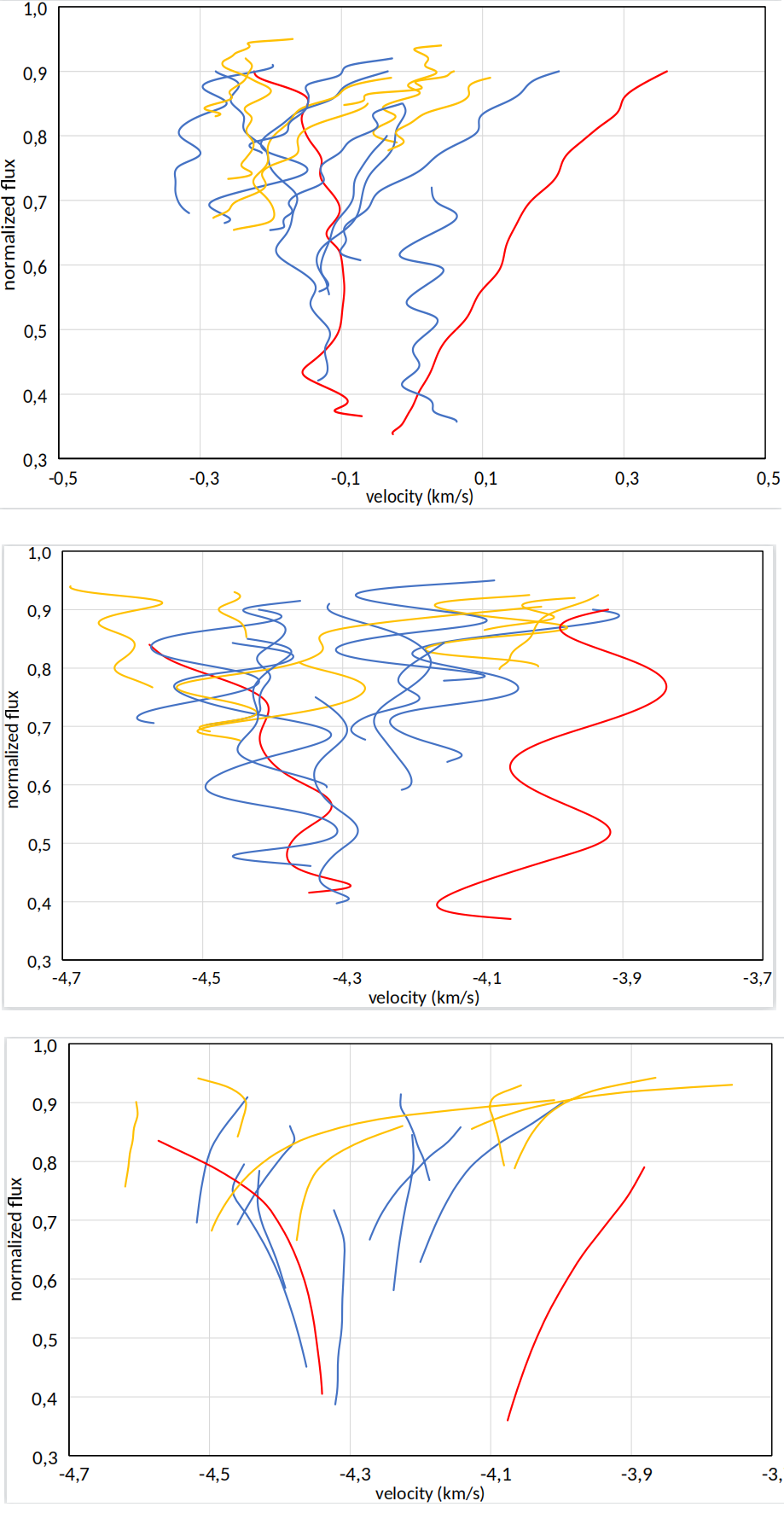
Fig. 2 (a) Bisectors from Arcturus-Hinkle in the range 7400 Å - 7500 Å, using the usual method of interpolating cubic splines between data points. Blue = iron, green = titanium, red = chromium. (b) Bisectors from Arcturus-UVES, with the same details as in Figure 2a. (c) Bisectors from Arcturus-UVES, with the method of adjusting a single polynomial to each spectral line. The color figure can be viewed online.
However, line asymmetry is measurable in UVES spectra (Dravins 2008) so we still use bisector tracing, but with a different technique. We fit a sixth-grade polynomial to each line profile, including as many data points as possible without impairing the quality of the fit (typically some 15 points), and draw the bisector from this polynomial. This method gives smooth bisectors (Figure 2c), which allow unequivocal positioning of the cores.
The number of data points to be included must be optimized for every line (Figure 3b); the correlation coefficient R 2 has a (slight) local maximum. If many more points are included, the polynomial is clearly incapable of modelling the line profile (Figure 3a); and if many fewer points are used, the point-to-point noise becomes noticeable (Figure 3c). Of course, when including n+1 data for a grade-n polynomial, the fit is “perfect” but does not filter out the random flux errors, and noise deformations are evident.
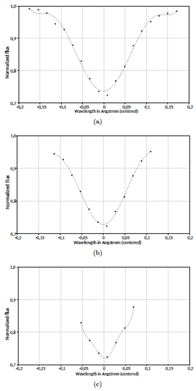
Fig. 3 (a) Profile of the 7489 Å Ti line in the UVES spectrum of HD209100, including 18 data points. The horizontal axis shows a relative wavelength scale in Å, and the dotted line is a 6th grade polynomial. The fit is inadequate because the number of points is too large. (b) The same as Figure 3a but including only 12 data points; this is the optimal number in this case. (c) The same as before but including only 7 data points; the fit is exact but the deformations are evident.
To estimate the uncertainty of the measured velocities, we varied the order of the polynomial and the number of data points included in the fit. Additionally, we compared for our 22 lines the velocities obtained from Arcturus-UVES with those from Arcturus-Hinkle. The differences have a standard deviation of 120 m/s. But this scatter is not random; it is the sum of a random error and a systematic error due to the difference in resolution of the two instruments. Plotting the difference in velocity against the slope of the bisectors, we find that the former has a spread of 65 m/s and the latter, spanning about 100 m/s, may be modeled and corrected.
3.2. Quantification of the Observed Redshift
To quantify the differential redshift of the Ti lines, we define the Mean Differential Redshift (MDR) for each star as the average velocity of the Ti lines minus the average of the Fe lines, divided by the standard deviation of the Ti velocities:
The reason for the “normalization” is that, when the Ti lines are more disperse, any shift of their average position is less significant statistically. For the mean velocities we use the simple average.
We compute the uncertainty of the MDR as the combination of the random uncertainties for the individual lines, which amount to 65 m/s. For NFe iron lines and NTi titanium lines, we get
Our line sample includes 9 Ti lines and 11 Fe lines; however, for computing MDR we exclude two high-redshift Ti lines (7432 Å and 7471 Å) which are illegible in some stars and blended in others; omitting them in all stars allows a more balanced comparison. Basically, then, NFe = 11 and NTi = 7; but these values may vary in some stars due to illegible lines. On the plots (Figures 4 to 7), all legible Ti lines are included, joined by line segments in a specific order as explained in § 5.
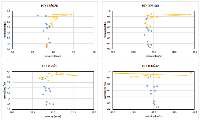
Fig. 4 Granulation diagrams of four MS stars. Ti lines are plotted in yellow, Fe lines in blue, and Cr lines in red. The excess redshift of titanium is evident, as is its gradual decrease. All our granulation diagrams cover a velocity range of 2 km/s. The large dispersion of Ti lines in HD 100623 may be caused by measurement errors due to their small depth. The color figure can be viewed online.
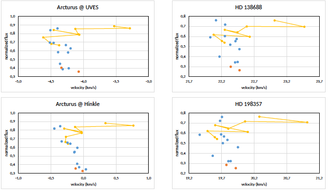
Fig. 5 Granulation diagrams for four RGB stars, including two from Arcturus. The smaller dispersion of the Fe lines in the Hinkle spectrum might be attributed to its higher resolution; but it is similar to the Fe distributions in the UVES spectra of the dwarf stars. The color figure can be viewed online.
4. Results
Due to our definition of MDR, the values may give the impression that the effect is smaller than it really is, for two reasons: We eliminated the two Ti lines with the largest redshift, thus reducing 〈VTi 〉; and the deepest Fe lines are redshifted by granulation (particularly in Arcturus-Hinkle), increasing 〈VFe 〉. For this reason, we show all the granulation diagrams.
4.1. Main Sequence
The clearest example of Ti redshift is the K5 dwarf HD 156026. From there, climbing the main sequence, the effect weakens gradually. The line with the largest shift in HD 209100 is at 7471 Å; this is due to a blend in some stars; it is excluded from the MDR computation in all stars. The granulation diagrams are shown in Figure 4. All results are summarized in Table 2.
Table 2 Measured redshit of Ti Lines*
| HD | Spectrum | B-V | MV | MDR | ΔMDR | |
|---|---|---|---|---|---|---|
| Dwarfs | 100623 | K0 V | 0,81 | 6,081 | -0,146 | 0,052 |
| 10361 | K2 V | 0,89 | 6,231 | 0,483 | 0,104 | |
| 209100 | K5 V | 1,06 | 6,885 | 0,608 | 0,267 | |
| 156026 | K5 V | 1,16 | 7,467 | 1,329 | 0,306 | |
| SG | 23249 | K0 IV | 0,92 | 3,759 | 0,220 | 0,065 |
| 138716 | K1 IV | 1,01 | 2,313 | 0,081 | 0,067 | |
| RC | 99322 | K0 III | 0,99 | 0,693 | 0,152 | 0,056 |
| 110458 | K0 III | 1,10 | 0,826 | -0,016 | 0,054 | |
| 140573 | K2 IIIb | 1,17 | 0,852 | 0,074 | 0,082 | |
| RGB | 124897-H | K1,5 III | 1,23 | -0,307 | 0,068 | 0,269 |
| 124897-U | K1,5 III | 1,23 | -0,307 | 0,162 | 0,141 | |
| 138688 | K2/4 III | 1,30 | -0,556 | 0,221 | 0,152 | |
| 198357 | K3 III | 1,39 | -0,608 | 0,166 | 0,130 | |
| 34055 | M4 III | 1,44 | -0,663 | 0,283 | 0,082 |
*Two MDR values are reported for HD 124897 (Arc-turus): The first is from the Hinkle spectrum, the second from UVES.
4.2. Red Giant Branch
The three K-type RGB stars are HD124897 (Arcturus), HD138688, and HD198357; for Arcturus we have two redshift data. The granulation diagrams are shown in Figure 5.
Our only M-type RGB star is HD 34055; its granulation diagram is presented in Figure 6. Here we clearly see the change of spectral class: Ti lines are deeper than Fe lines.
4.3. Red Clump and Subgiants
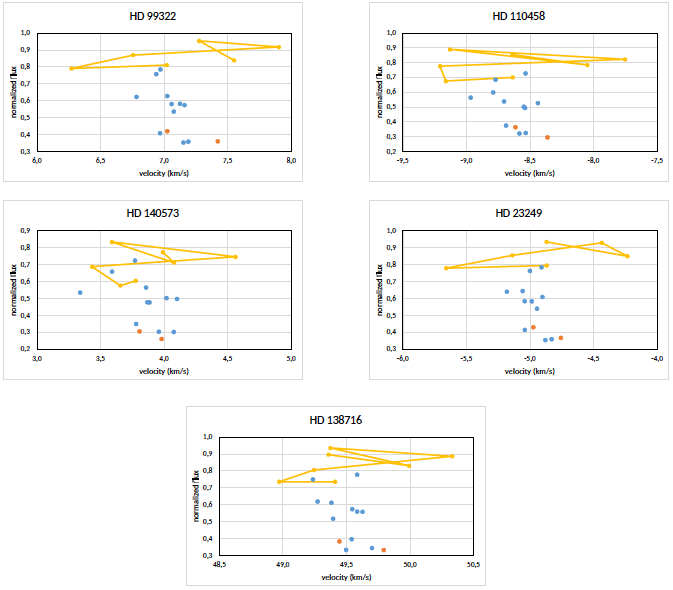
Finally, Figure 7 shows the granulation diagrams of our three red clump stars and two subgiants.
4.4. Color Dependence
It would be natural to inquire how MDR depends on basic stellar parameters such as color index or absolute magnitude. Within each class, the variation of absolute magnitude is rather small; therefore we show the relation between observed redshift and color (Figure 8).
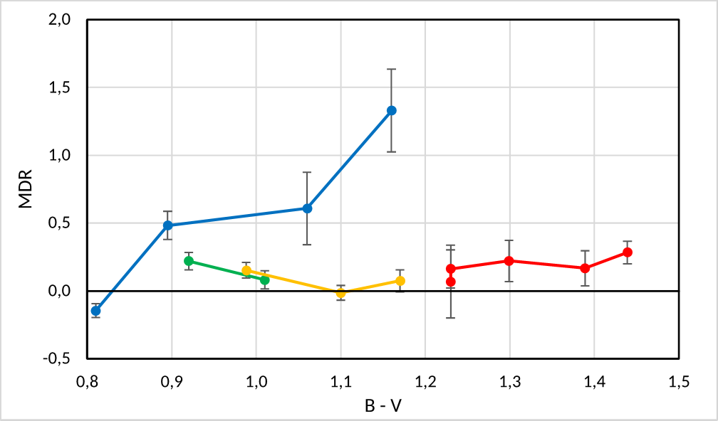
Fig. 8 Color dependence of Ti redshift. The colors indicate the groups as in Figure 1. Blue: main sequence; green: subgiants; yellow: red clump; and red: red giant branch. The color figure can be viewed online.
5. Discussion
In search of an explanation for the differential redshift, we studied the temperature-dependence of these spectral lines, extracting synthetic spectra from VALD for eleven stellar temperatures between 3500 K and 6000 K and plotting these theoretical depths (Figure 9).
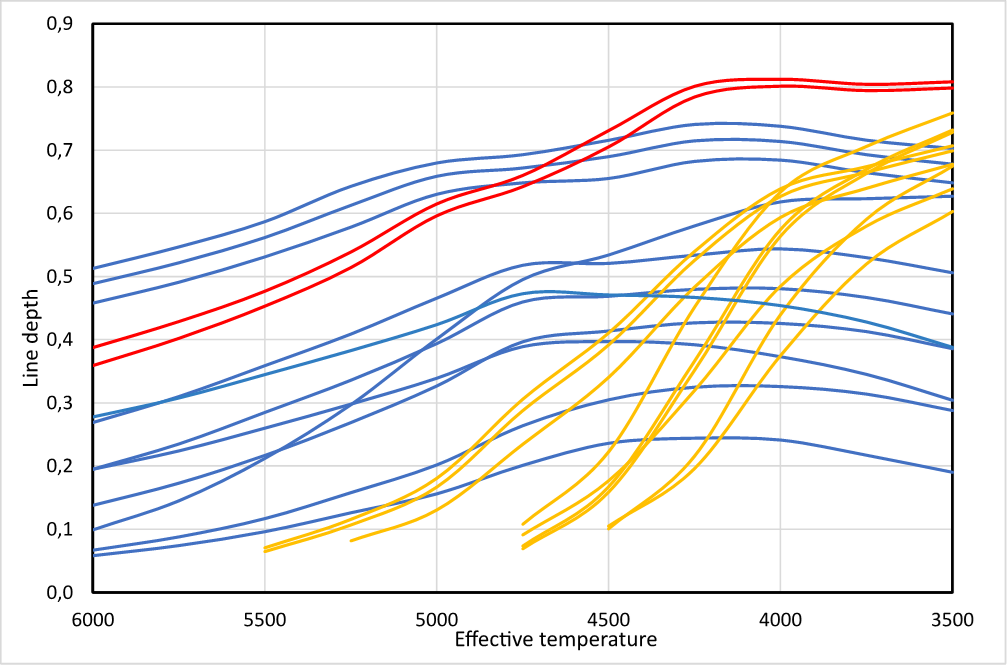
Fig. 9 VALD Line depth versus stellar temperature for Fe (blue), Cr (red) and Ti lines (yellow). The color figure can be viewed online.
It is evident that Ti lines weaken towards hotter stars much faster than Fe lines. This is due to ionization of Ti in hotter stars. We suggest that this thermosensitivity is also responsible for the redshift of Ti lines as compared to Fe lines. As a further evidence for the relation between these two phenomena, we discriminate between the Ti lines: the lines which disappear faster as the effective temperature increases, i.e. the most thermosensitive lines, are also the lines with a greater differential redshift. To make this more apparent we number the Ti lines in Figure 9 from top left to bottom right, roughly between 4000 K and 4500 K. These numbers are given in Table 1 in the column labeled “Thermo”. In all the granulation diagrams we linked the Ti points by line segments in this order. Lines 1, 2 and 3 are the strongest or deepest; in most diagrams, these lower numbers cluster toward the left while higher numbers are more to the right. In other words, the differential redshift of individual Ti lines correlates roughly with the thermodependence shown in Figure 9.
We propose an explanation of the differential redshift based on granulation. On the star’s photosphere are bright spots of hot, rising gas separated by darker lanes of cool, sinking material. The most thermosensitive lines, which disappear faster as stellar effective temperature increases, originate mainly in the cool intergranular lanes, rather than in the hot granules where line formation is impaired by Ti ionization. The latter regions are blueshifted by upwelling convection currents, while the former are redshifted as the cool material sinks back into the star. This phenomenon affects Ti lines more than Fe lines, and some Ti lines more than others.
We conclude that the differential redshift is basically a sign of granulation. Three spectroscopic signatures of stellar granulation have been published earlier (Gray 2009): overall line broadening, line profile asymmetry (bisector shape), and a core blueshift which correlates inversely with line depth. The differential redshift of the Ti lines is another such signature.
We are aware that our sample is very small and cannot allow general conclusions.
The spectral region of 7400 Å - 7500 Å which we chose mainly to avoid TiO bands, turned out to include a CN band which is prominent in several of our stars. The Ti lines 7432 Å and 7471 Å are notably affected in some stars. We checked if the differential redshift is not an artifact of CN blends. On the contrary, we found a strong inverse correlation between the CN strength and Ti redshift. We conclude that the CN band partially masks the differential Ti redshift.
The differential redshift of a certain chemical species will broaden some granulation diagrams. A detailed characterization of this effect may help to reduce uncertainties in granulation studies and radial velocity measurements. Another possible strategy is to use only Fe lines.
The greater redshift of the weaker Ti lines constitutes the upper part of the “C” shape of the granulation diagram for cool stars. The same effect is expected for iron lines, but for shallower lines, or deeper layers in the photosphere. This means that the granulation diagram is not a unique curve, but rather one curve is needed for each element.
Considering this, it is to be expected that the differential redshift disappears at the granulation boundary (Gray & Nagel 1989), at the blue side of which the granulation plots resemble the symbol “Ↄ” or inverse “C”. The effect is expected to increase from the boundary toward cooler stars, particularly giants where intergranular lanes occupy a relatively larger area.
We appreciate the valuable suggestions and corrections of the referee.

