


 nueva página del texto (beta)
 Inglés (pdf)
 Artículo en XML
 Referencias del artículo
 Enviar artículo por email
 Citado por SciELO
  Similares en
SciELO
Similares en
SciELO 
 Permalink
1. INTRODUCTION
The formation and evolution of galaxies at high redshift strongly determined the progression of the epoch of reionization (EoR). The hierarchical model for structure formation provides a scenario where small dark matter halos (≈106Mʘ) at z≈30 reached a critical temperature to agglomerate baryons, and formed stars (Tegmark et al. 1997), initially metal-free (POP III). However, these first stars evolved and consumed their fuel quickly and produced the first supernova explosions. With them, the chemical pollution of the intergalactic medium (IGM) began (Matteucci & Calura 2005). Consequently, a new generation of stars (POP II) formed the first black holes in the Universe. Interestingly, metals in POP II stars supplied an additional cooling source; therefore, these structures were less massive and had longer lives than metal-free stars. The interaction of the collapsed systems in the Universe and the IGM is described through feedback models that account for winds that spread out chemical elements and vary the ionization state of free hydrogen.
Using Hubble Space Telescope imaging, Robertson et al. (2015) measured the abundance and luminosity distribution of early galaxies and provided a constraint for the observed star formation rate (SFR). However, the largest compilation to date for the SFR was presented by Madau & Dickinson (2014). Later works by Oesch et al. (2015); McLeod et al. (2015); Finkelstein et al. (2015); Song et al. (2016); Oesch et al. (2018); Ishigaki et al. (2018); Bhatawdekar et al. (2019); among others, have complemented our survey of galaxies at early times, pushing the detections to very faint objects at higher redshifts (z ≈ 11; Robertson 2021).
On the other hand, theoretical models have a threefold purpose: (i) match the observations available for the synthetic galaxies and their environment; (ii) provide a physical description of the star formation process at all times, and (iii) interpolate -when possible- the progression of galaxies and their properties in time. There are multiple models that reproduce the star formation history of galaxies at early times, focusing on specific physical processes, among them: Angus (AustraliaN Gadget-3 early Universe Simulations, Tescari et al. 2014); the Renaissance suite (with the AMR code Enzo, O’Shea et al. 2015); Eagle (Evolution and Assembly of GaLaxies and their Environments, Crain et al. 2015; Schaye et al. 2015); CROC (Cosmic Reionization on Computers, Zhu et al. 2020); the Obelisk simulation (Trebitsch et al. 2020); L-Galaxies 2020 (Henriques et al. 2020; Yates et al. 2021a); Flares (First Light And Reionisation Epoch Simulations, Lovell et al. 2021; Vijayan et al. 2021); Astraeus (semi-numerical rAdiative tranSfer coupling of galaxy formaTion and Reionization in N-body dArk mattEr simUlationS, Hutter et al. 2021).
With the advent of the James Webb Space Telescope (JWST) shortly, we will reach an unprecedented understanding of the first light and the reionization, as well as the assembly of galaxies (Gardner et al. 2006). The expectation is that JWST will observe galaxies out to z > 12 and even at z ≈ 15 (depending on their brightness). It will provide a uniform census of galaxies in the redshift range of 7 - 12 and extend the observed cosmic star formation evolution at a level not achievable by Hubble (Finkelstein 2016). In addition, JWST will: detect stars with very low metallicity (10−3 Z ), set constraints of the top-heavy IMF, provide an estimate of the escape fraction of ionizing photons of galaxies, and allow for a robust investigation of the UV luminosity function at high redshift (Atek et al. 2015 found a steep faint-end slope at z ≈ 7). Theoretical works such as UniverseMachine by Behroozi et al. (2020), IllustrisTNG with dust modeling (Vogelsberger et al. 2020) or Williams et al. (2018) -that creates a mock catalog of galaxy populations from the UV to the near-infrared- anticipate future observations from the instrument and provide a realistic (yet conservative) forecast of the galaxy assembly at redshifts up to 15.
The paper is presented as follows: § 2 gives an overview of our numerical simulations and the physical modules implemented to recreate the structure formation at high redshift. Also, we briefly present a description of other numerical simulations considered to evaluate the performance of our models. § 3 shows a series of statistics for galaxy and halo properties in the simulations at 4 < z < 8. We also compare our theoretical predictions with observational data available to-date and to the largest compilation of high-resolution cosmological models in this redshift range. We establish a connection between the galaxy properties and their hosting dark matter halo and show a self-consistent chemical enrichment in the models. § 4 discusses future scenarios where our conclusions can be tested, as well as the strengths and caveats of our models. Finally, § 5 summarizes the findings and conclusions of this study.
2. THE NUMERICAL SIMULATIONS
This work relies on a set of high-resolution hydrodynamical simulations at high redshift (4 < z < 8), initially presented in García et al. (2017b). The model is based on a customized version of the smoothed particle hydrodynamics (SPH) code Gadget-3 (Springel 2005), with a spatially flat cosmology ΛCDM model and cosmological parameters Ω0m = 0.307, Ω0b = 0.049, ΩΛ = 0.693, n s = 0.967, H 0 = 67.74 km s−1Mpc−1 (or h = 0.6774) and σ8 = 0.816. A summary of the numerical simulations is shown in Table 1.
TABLE 1 OVERVIEW OF THE SIMULATIONS USED IN THE PAPER*
| Simulation | Box size (cMpc/h) |
Comoving softening (ckpc/h) |
Mgas (×105Mʘ/h) |
MDM (×106Mʘ/h) |
| Ch18512MDW | 18 | 1.5 | 5.86 | 3.12 |
| Ch 18 512 MDW mol | 18 | 1.5 | 5.86 | 3.12 |
| Ch 18 512 EDW | 18 | 1.5 | 5.86 | 3.12 |
| Ch 18 512 EDW mol | 18 | 1.5 | 5.86 | 3.12 |
| Ch 12 512 MDW mol | 12 | 1.0 | 1.74 | 0.925 |
| Ch 25 512 MDW mol | 25 | 2.0 | 15.73 | 8.48 |
*The first column corresponds to the name of the run, the second one to the box size. The third column lists the comoving gravitational softening length. Columns 4 and 5: the gas and DM particle masses. Note that all runs have the same initial number of gas and DM particles (2 × 5123). The acronyms MDW and EDW stand for momentum- and energy-driven winds feedback prescriptions, and mol at the end of the run’s name indicates the presence of low-temperature metal and molecular cooling. The fiducial model is highlighted in bold in the first row: Ch 18 512 MDW.
The numerical models are complemented with an algorithm that identifies collapsed structures, so-called parallel Friends-of-Friends (FoF), and a parallel SUBFIND algorithm to identify substructures within FoF halos.
The mechanism for which star-forming gas particles turn into star-type particles by a stochastic process was first proposed by Katz et al. (1996) and later discussed in Springel & Hernquist (2003); Tornatore et al. (2007).
Thus, our model produces self-consistently chemical enrichment based on the stochastic scheme for star formation. The module follows the evolution of hydrogen, helium, and nine elements up to iron, delivered from SNIa and SNII and intermediate-mass stars. Importantly, stars with masses m ≤ 40M explode as supernovae before turning into a black hole. Conversely, stars above such threshold collapse into a black hole without experiencing the supernova stage, contributing to the feedback process, but not to the chemical evolution in the simulations. The overall state of a simple stellar population depends on the lifetime function (Padovani & Matteucci 1993), the stellar yields, and the initial mass function (IMF).
The stellar yields account for the amount of metals released by each source during the stellar evolution: SNIa (Thielemann et al. 2003), SNII (Woosley & Weaver 1995) and low- and intermediate-mass stars. Moreover, the solar metallicity layers follow results from Asplund et al. (2009).
The cooling processes that allow the gas to form stars include atomic, metal-line cooling (Wiersma et al. 2009), as well as low-temperature cooling by molecules and metals (Maio et al. 2007; Maio & Tescari 2015).
On the other hand, this work builds on a multi-sloped IMF (Chabrier 2003) that accounts for massive POP II and, to some extent, to POP III stars, which significantly contribute to the first stages of the star formation processes and the hydrogen reionization.
Our numerical simulations implement galactic winds to regulate the star formation process, the dispersion of metals from galaxies to the intergalactic medium (IGM), and prevent overcooling of the gas (Springel & Hernquist 2003). Such feedback mechanisms expel material and balance the temperature among neighbor gas particles, allowing physical processes to occur. There are two kinetic supernova-driven winds considered in this work: energy- (EDW; Springel & Hernquist 2003) and momentum-driven winds (MDW; Puchwein et al. 2013), and AGN feedback (Springel et al. 2005; Fabjan et al. 2010; Planelles et al. 2013). The latter type of feedback is essential at low redshift (z ≈ 2) when massive halos are more numerous and massive.
In this work, both EDW and MDW supernova outflows are implemented, with a fixed fiducial velocity vfid = 600 km/s. The main assumption in the former prescription for the winds is the proportionality between the star formation rate Ṁ* and the mass-loss rate due to winds Ṁ w , through the relation Ṁw = ηṀ*. The factor η is defined as the wind mass loading factor and quantifies the efficiency of the wind to expel material out of the source cell.
The kinetic energy of the wind and the halo circular velocity allow us to establish a numerical relation between wind mass-loading factor η and vw 1:
Nonetheless, Puchwein et al. (2013) show that the star formation rate Ṁ* and the mass expelled by supernova winds Ṁ
w
do not necessarily have a linear relation. Instead, a more natural assumption would be a mathematical relationship for the star formation rate of the galaxy and the winds’ momentum flux. In such case,
It is worth mentioning that the wind velocity v w has the same functional form as in the energy-driven winds feedback. Yet, their efficiencies η behave in distinctive ways because of the scaling with v w.
On the other hand, different authors have shown that AGN feedback is critical to regulate the star formation rate history, gas accretion, stellar evolution, and metal enrichment when the Universe has evolved for 10 billion years (i.e., z ≈ 2), at the peak of the star formation and consequently, the most significant quasar activity in the history of the Universe.
Nevertheless, Tescari et al. (2014) present an extensive discussion of the negligible effect of AGN feedback at the redshifts of interest of this work. Two main factors determine that AGNs do not play an essential role at high redshift: (i) the galaxies are still experiencing their first stages of star formation; hence, very few super-massive black holes have formed at this time; (ii) dark matter halos are still growing by mergers; thus, AGNs (if existing) are rare, and so are their feedback mechanisms.
Other Numerical Simulations
In order to convey a successful comparison of the predictions from this set of simulations with current theoretical models, we briefly summarize the main features of each of the mock cosmological boxes, highlighting their resolution and box sizes.
-
UniverseMachine
As described in Behroozi et al. (2020), the UniverseMachine is based on the Very Small MultiDark-Planck (VSMDPL) simulation, a modified version of GADGET- 2 with a flat ΛCDM model and h = 0.68. This model was run from z = 150 to 0, in a cube size of 160 cMpc/h with 38403 particles, allowing it to reach a gas mass of 9.1 × 10⁶Mʘ, a numerical resolution of 2 ckpc/h at z > 1 and resolved dark matter halos with 100 particles (i.e., above 109Mʘ). The latter property of the UniverseMachine makes it suitable to appropriately describe halos at high redshift and to foresee the characteristics of undetected galaxies at the epoch of reionization.
-
L-Galaxies 2020
This semianalytical model of galaxy evolution (Henriques et al. 2020) is run on the Millennium-II simulations in a box of ≈ 96.1 Mpc/h side. It only contains dark matter particles (the baryonic physics is implemented through effective modules that are easily adapted), reaching a broad coverage at the cosmological level. The dark matter particles have a mass resolution of 7.7 × 10⁶Mʘ/h. The model is scaled to the Planck 2013 cosmology with h = 0.673. L-Galaxies 2020 currently has two distributions: Default model or DM, first described in Henriques et al. (2020), assumes that 70% of the metal content is released by supernova is instantly mixed with the local interstellar medium (ISM) before being expelled out of galaxies via SN winds. Instead, the Modified model -MM- (Yates et al. 2021a) adopts a chemical pollution prescription where up to 90% of metals produced in supernova explosions are moved directly to the circumgalactic medium (CGM) without passing by the ISM. These two complementary scenarios cover a wide range of CGM enrichment schemes, likely to occur in real galaxies.
-
Eagle
Evolution and Assembly of GaLaxies and their Environments (Eagle) is a hydrodynamical suite of cosmological simulations run in a modified version of Gadget- 3 (Crain et al. 2015; Schaye et al. 2015). The model’s main strength is the galaxy growth and evolution, and it includes similar prescriptions and modules as the ones implemented in our numerical simulations. For this paper, we will only focus on their largest volume ‘L100N1504’ cube, with 67 (Mpc/h)3 box-size and 2 × 15043 particles (dark matter+gas). The initial mass is 1.2(6.6)×106Mʘ/h for baryons (and dark matter). The assumed cosmology is Planck 2013 with h = 0.6777, and their supernova feedback is EDW.
-
TNG100
IllustrisTNG is a set of gravo-magnetohydrodynamical simulations based on the Illustris project (Nelson et al. 2018; Pillepich et al. 2018; Naiman et al. 2018; Marinacci et al. 2018; Springel et al. 2018). TNG (The Next Generation) has a standard configuration for three different volumes: 35, 75, and 205 cMpc/ h of side length -TNG50, TNG100, and TNG300, respectively-. The first box size involves the largest resolution, instead of TNG300, which covers a more vast cosmological region at the expense of reducing the gravitational softening. Each simulated box has different levels of resolution (moving from 1 to 3-4, with decreasing numerical resolution and lighter simulation outputs). The assumed cosmology is Planck 2015 with h = 0.6774. In particular, for the comparison intended in this work, we only consider the TNG100-1 run, with 2×18203 particles, and average cell masses of 7.5 × 10⁶Mʘ and 1.4 × 10⁶Mʘ for dark matter and gas, respectively.
-
Flares
First Light and Reionisation Epoch Simulations (Flares) is a suite of zoom simulations that focuses on the typical overdensities reached during the epoch of reionization. The models are presented and discussed in Lovell et al. (2021); Vijayan et al. (2021), and they are a re-simulated version of Eagle with a total volume of (3.2 cGpc)3 -dark matter only-. The dark matter particles have a mass of 8.01 × 10¹⁰Mʘ/h. Smaller regions of 15 Mpc/h in radius are re-computed with a full hydrodynamical treatment (about our boxes in size) from z = 10 down to z = 4.67 with the Eagle galaxy formation scheme. Flares assumes Planck 2014 cosmological parameters with h = 0.6777, and the same configuration as the Eagle reference run (100 cMpc) with 9.7 and 1.6 × 10⁶Mʘ initial masses for dark matter and gas particles, respectively, leading to a numericalresolutionof2.66ckpc(between the gravitational softening reached by our synthetic boxes with 18 and 25 cMpc/h).
3. GALAXY PROPERTIES IN OUR SIMULATIONS
Following the assumptions from previous section, AGN feedback is not implemented in our simulations (Tescari et al. 2014). The simulations were anchored at z = 8, and observables such as the cosmic star formation rate and the galaxy stellar mass function were used to calibrate the mass loading factor for the winds vfid = 600 km/s, and match the observations at the time when García et al. (2017b) was published. Hence, the SFR (z = 8) and the stellar mass function are not predictions of the model.
3.1. Halo Occupation Fraction
The halo occupation fraction presents the distribution of dark matter halos with chemically enriched starparticles at a particular redshift, as a function of the halo mass. We present the halo occupation fraction in the fiducial model Ch 18 512 MDW in Figure 1, including mass bins of log(M h/Mʘ) = 0.1. It is worth noting that we only take into account halos above the mass resolution M h,min = 1.48 x 10⁹Mʘ.

Fig. 1 Halo occupation fraction in the simulation Ch 18 512 MDW (our fiducial run). The distributions show the percentage of dark matter halos containing formed stars at z = 8, 7, and 6 (light, navy, and dark blue lines, respectively). The color figure can be viewed online. vfid = 600 km/s, and match the observations at the time when García et al. (2017b) was published. Hence, the SFR (z = 8) and the stellar mass function are not predictions of the model.
The distribution in Figure 1 reaches its maximum occupation at M h ≈ 1 ≈ 1010Mʘ for z = 8, 7, and 6, which is consistent with the hierarchical model of structure formation. Dark matter halos with masses below 109Mʘ contain less than 470 dark matter particles, then they cannot be considered virialized, and the star formation in such regions is disfavoured for two reasons: first, they are unresolved, and they do not efficiently experience atomic cooling; hence, gas is collisionally excited and less likely to form structure in the dark matter wells until it cools down. On the contrary, halos with large masses (≥ 1010Mʘ) preferentially form stars, but they are rare on the simulations at high redshift. Although scarce, dark matter halos with large masses present a non-negligible occupation of chemically enriched stellar populations.
At z = 6 (dark blue line), when the Universe has evolved for ≈ 360 Myr from the start of the simulations (z = 8), the highest probability of finding fully occupied halos occurs at M h ≈ 1 x 10¹⁰Mʘ. The latter result indicates that halos in the simulation have grown in mass during this period and, consequently, also the cosmic star formation rate.
3.2. Stellar-to-Halo Mass Function
Another observable that we check in our models is known as the galaxy stellar-to-halo virial mass function, presented in Figure 2 for the fiducial run Ch 18 512 MDW, at z = 8 and 6.

Fig. 2 Galaxy stellar-to-halo virial mass function in our reference model Ch 18 512 MDW. The graph displays the distribution of masses above the threshold for this simulation box-size at redshifts z = 8 and 6 (corresponding to light and dark blue stars, respectively). For comparison, the predicted trends from UniverseMachine (Behroozi et al. 2020) are shown at z = 8 (dark red circles) and z = 6 (red dots). Grey dashed lines indicate constant stellar functions f ∗ = M ∗/M h, ranging from 10−4 (bottom) to 10−1 (top). The color figure can be viewed online.
Figure 2 presents the distribution of the stellar-tohalo mass for each galaxy in the fiducial simulation above the mass resolution threshold (> 109Mʘ or equivalently, more than 470 dark matter particles). Simulated galaxies follow a trend of 10−2, and at the high mass end, f ∗ moves to 10−1. f ∗ grows with redshift, with more galaxies with large stellar masses at z = 6. This result is also seen in numerical simulations such as Astraeus (Hutter et al. 2021), with M h = 109.5−10Mʘ corresponding to stellar masses ≈ 107.5−8Mʘ during the epoch of reionization. Moreover, O’Shea et al. (2015) display this distribution (Figure 2, left), but they stack all the galaxies in their realizations up to their final redshifts. The Renaissance simulations describe galaxies that are evolving during the progress of reionization; therefore, they account for halo masses down to 7 × 10⁶Mʘ (halos with formed stars). Their plot is not directly comparable with Figure 2 because the mass range covered by their simulations differs from ours. Still, galaxies around 109Min their work show the same difference of two orders of magnitude in M h/M s. Recent observations by Stefanon et al. (2021) reveal the same ratio of two orders of magnitude for stellar-to-halo mass ratios (see Table 7 in their work). They emphasize that there is no significant evolution in the observed stellar-to-halo mass function for galaxies in the first Gyr of cosmic time. The latter conclusion is consistent with Figure 2. Instead, predictions by Behroozi et al. (2020) are an order of magnitude below the trend of our fiducial simulation, at z = 8 and 6. However, we cannot provide a clear explanation for this discrepancy since UniverseMachine is calibrated to resolve virialized halos up to z ≈ 15, but the ratio predicted by their simulation is off compared with other simulations at z = 6 - 8 (including ours).
It is worth mentioning that we only calculate the stellar-to-halo mass function for the fiducial model Ch 18 512 MDW because there is minimal variation in the range of masses resolved by our simulations due to our small boxes (12, 18, and 25 cMpc/h). Thus, the trend shown in Figure 2 is barely affected by changes in the box size.
3.3. Galaxy Stellar Mass Function
One can also count the number density of galaxies formed inside the virialized halos per unit volume V per stellar mass bin ∆M (Weigel et al. 2016). This observable is known as the galaxy stellar mass function, and it is given by:
The analytical form that describes the galaxy stellar mass function is commonly described using a Schechter function (Schechter 1976), as follows:
The exponential term in the expression above shows the evolution for the high- and low-mass and the fore-most right term a power-law behavior as a function of the stellar mass.
We present the best fit parameters and corresponding errors for the galaxy stellar mass functions at z = 8, 7, and 6 for three of our models with same configuration (MDW and no molecular cooling) with box sizes of 12, 18, and 25 cMpc/h, in Table 2. We derive these parameters with an adapted version from python routine emcee. Table 2 also shows the Schechter function parameters from Duncan et al. (2014), Grazian et al. (2015), Bhatawdekar et al. (2019) and Stefanon et al. (2021).
TABLE 2 BEST FIT SCHECHTER FUNCTION PARAMETERS AND UNCERTAINTIES FOR THE GALAXY STELLAR MASS FUNCTION Φ(M)*
| log10M∗ | α | Φ∗ (10−5Mpc−3) | |
| z ≈ 8 | |||
| Stefanon et al. (2021) |
|
|
|
| Bhatawdekar et al. (2019) |
|
|
|
| Ch 18 512 MDW | 10.34 ± 0.02 | −2.20 ± 0.05 | 0.092 ± 0.005 |
| Ch 12 512 MDW | 9.25 ± 0.02 | −2.15 ± 0.06 | 0.870 ± 0.005 |
| Ch 25 512 MDW | 10.55 ± 0.02 | −2.30 ± 0.07 | 0.098 ± 0.005 |
| z ≈ 7 | |||
| Stefanon et al. (2021) |
|
|
|
| Bhatawdekar et al. (2019) |
|
|
|
| Grazian et al. (2015) |
|
|
|
| Duncan et al. (2014) |
|
|
|
| Ch 18 512 MDW | 10.61 ± 0.02 | −1.95 ± 0.04 | 0.67 ± 0.03 |
| Ch 12 512 MDW | 10.72 ± 0.02 | −1.92 ± 0.04 | 0.60 ± 0.03 |
| Ch 25 512 MDW | 10.51 ± 0.02 | −2.10 ± 0.05 | 0.72 ± 0.03 |
| z ≈ 6 | |||
| Stefanon et al. (2021) |
|
|
|
| Bhatawdekar et al. (2019) |
|
|
|
| Grazian et al. (2015) |
|
|
|
| Duncan et al. (2014) |
|
|
|
| Ch 18 512 MDW | 10.41 ± 0.02 | −2.01 ± 0.05 | 1.20 ± 0.03 |
| Ch 12 512 MDW | 10.42 ± 0.02 | −2.02 ± 0.05 | 1.15 ± 0.03 |
| Ch 25 512 MDW | 10.40 ± 0.02 | −2.05 ± 0.05 | 3.20 ± 0.03 |
*For each redshift, we find the best parameters for the fiducial model and two equivalent runs with the same setup, but 12 and 25 cMpc/h box side.
One highlight from Table 2 is that the slope of the galaxy stellar mass function at z = 6 - 8 remains constant, and in all the cases presented, is close to the value −2. These findings are consistent with the observational constraints also shown in Table 2.
The evolution of the galaxy stellar mass function from z = 8 to 6 is displayed in Figure 3. Remarkably, the galaxy stellar mass function Φ at z = 8 was set to match observations by Song et al. (2016) and to calibrate the mass loading factor of the simulations vfid. However, the theoretical trends agree well with the best fit at z = 8 by Bhatawdekar et al. (2019) and with the most recent Spitzer/IRAC observations by Stefanon et al. (2021), which is quite reassuring since the observational detections came after our simulations.
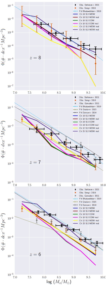
Fig. 3 Simulated galaxy stellar mass function at z = 8, 7 and 6 in the top, middle and bottom panels. Theoretical predictions from our models are compared with observations by Stefanon et al. (2021) as black diamonds, Song et al. (2016) as orange circles and González et al. (2011) as grey circles, and the best fits proposed Bhatawdekar et al. (2019), Grazian et al. (2015) and Duncan et al. (2014) as light blue, olive and black dotted lines, respectively. The parameters of the Schechter function (4) for each model are presented in Table 2. The color figure can be viewed online.
The predicted galaxy stellar mass functions at z = 8, 7, and 6 are compatible with the observational data at high z. Nonetheless, the simulations slightly differ from the galaxy stellar mass function reported by Song et al.(2016) and González et al. (2011) in the high mass end at z = 6, mainly because massive galactic halos are scarce in the simulations at these redshifts; thus, high-mass galaxies are rare. Larger synthetic boxes could alleviate this mass bias (for instance, Flares or UniverseMachine).
On the other hand, results with Flares (Lovell et al. 2021; Vijayan et al. 2021, supported by a vast cosmological box, that at z = 5 and 6, reach stellar masses up to 1011Mʘ), claim that the galaxy stellar mass function must be fitted with a double-slope Schechter function with a knee at Ms = 1010Mʘ. They back the latter argument with recent observational constrains from Stefanon et al. (2021). Nevertheless, our small boxes do not allow us to test this range of mass (Ms,max ≈ 109.8Mʘ in our largest realization; hence, we keep a single-slope fit). One of the motivations for the Lovell et al. (2021) work was to extend the range of stellar masses and the number of resolved galaxies reached by the Eagle simulation. Our cosmological runs have similar modules, box sizes, and an analogous configuration as Eagle; therefore, tests related to galaxy observables must be done with Eagle -or equivalent hydrodynamical simulations. Instead, this particular conclusion derived by Lovell et al. (2021) is out of the reach of our simulations.
3.4. Halo Mass Function
In order to characterize the galaxies in the simulations, the halo mass functions at redshifts z = 8, 7, and 6 are presented in Figure 4, in light, navy, and dark blue lines, respectively. This quantity is computed with systems above the mass resolution limit (a resolved halo in the simulation contains ≈ 470 dark matter particles, or equivalently, a minimum mass M h,min = 1.48 × 10⁹Mʘ for boxes of 18 Mpc/h side length). Whenever a galactic halo is below this mass threshold, the object is considered unresolved and is excluded from the statistics.
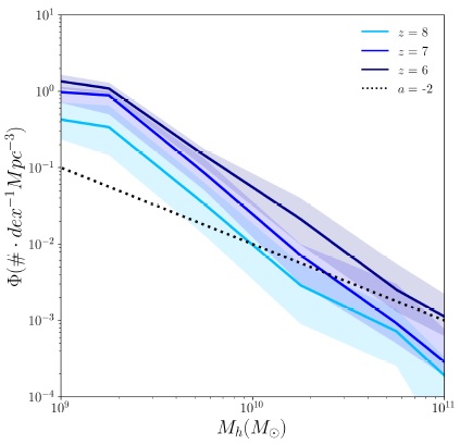
Fig. 4 Halo mass functions at z = 6, 7, and 8 in dark, navy, and light blue. We include shaded regions corresponding to Poisson errors for the fiducial run Ch 18 512 MDW. As a reference, we show a constant power-law slope α = −2 for galaxies at high redshift, as a dotted black line. The color figure can be viewed online.
The evolution of the mass function for dark matter halos is computed only with the fiducial model Ch 18 512 MDW since the number of resolved galaxies is almost independent of the feedback mechanisms or the cooling processes implemented in the simulations. As a reference, a dotted black line is presented on top of our predictions in Figure 4, indicating a constant faint-end slope α = −2.
Theoretically, the number density of halos follows the relations
We support the latter claim based on the results described in previous sections. The stellar-to-halo mass ratio (Figure 2) shows little evolution of the mass ratio at z = 8 to 6 (regardless of the increasing number of halos that form galaxies with time). On the other hand, the galaxy stellar mass function (Table 2 and Figure 3) indicates that the slope is close to −2 during the time frame described by the simulations. Since the halo masses, M h are two orders of magnitude larger than the stellar masses M s -this ratio stays constant at the tail of the reionizationand the slope for the stellar mass function is −2, with almost no variation in time, the value of the slope of the halo mass function is consistent with −2.
3.5. Star Formation Rate Density
The star formation rate is the mass of the new stars in the simulation, measured in the total volume per year. It is commonly assessed by galaxy surveys or derived from studies with luminosity functions. There are two ways to compute the cosmic star formation rate in the numerical runs: (i) adding up the star formation of each gas particle, per comoving volume V; or (ii) recovering the SFR estimate for galaxy groups from the FoF catalog.
Figure 5 shows the cosmic star formation rate in our simulations at 4 < z < 8. The left panel shows the total SFR (including contributions from all the collapsed objects inside the box). Conversely, the right panel displays the same observable, but this time, applying a cut in mass; thus, only the most luminous galaxies are taken into account in the calculation. This mass threshold responds to the resolution achieved by our telescopes that only detect the most luminous galaxies (in particular, at high redshift). Current instruments do not detect the faintest objects; therefore, their SFR cannot be inferred with that method. Consequently, there is an excess in the star formation rate predicted by the simulations -on the left- to observational data. The discrepancy between the calculated and the observed SFR is corrected in the right panel by imposing a luminosity cut MUV < −17 (corresponding to a minimum SFR > 0.331 Mʘ/yr and the absolute magnitude set by Hubble observations). When we impose the latter criterion to the simulations, the predicted SFR agrees well with the observations to-date (except for data points measured by Steidel et al. (1999) and Ouchi et al. (2004) that do not account for dust corrections).

Fig. 5 Cosmic star formation rate density in the redshift range of 4 < z < 8. The predictions from the simulations are compared with observations from Bhatawdekar et al. (2019) shown as brown diamonts, Driver et al. (2018) as yellow squares, Bouwens et al. (2015) as orange circles (with dust corrections), Cucciati et al. (2012) as an olive pentagon, Hildebrandt et al. (2010) as a green inverted triangle, Bouwens et al. (2009) as a pink square, Ouchi et al. (2004) as cyan triangles and Steidel et al. (1999) as a grey diamond. In the left panel, the SFR in the simulations is computed including all objects in the box per unit volume. On the right, the observable is limited to masses with the luminosity cut of MUV < −17, equivalent to a minimum SFR of > 0.331Mʘ/yr, following the observational constraints of our current telescopes. The color figure can be viewed online.
Interestingly, data from Driver et al. (2018) and Bhatawdekar et al. (2019) had not been published when our simulations were run, but most of the models are in agreement with these observations.
On the other hand, the cosmic SFR reported by Finkelstein (2016) -with a corresponding comparison with Madau & Dickinson (2014)- shows an increment of 1 dex in their reference model, consistent with findings from this work with the mass cut MUV < −17 (right panel of Figure 5).
Figure 6 shows a compilation of theoretical predictions for the cosmic star formation rate by UniverseMachine(Behroozietal.2020), L-Galaxies 2020(Henriques et al. 2020; Yates et al. 2021a), Flares (Lovell et al. 2021; Vijayan et al. 2021), TNG100 (Nelson et al. 2018; Pillepich et al. 2018; Naiman et al. 2018; Marinacci et al. 2018; Springel et al. 2018), Eagle (Crain et al. 2015; Schaye et al. 2015) and our models.

Fig. 6 Cosmic star formation rate density in the redshift range of 4 < z < 8. The predictions from our models are compared with the calculated SFR with the UniverseMachine (Behroozi et al. 2020), L-Galaxies 2020 (Henriques et al. 2020; Yates et al. 2021a), Flares (Lovell et al. 2021; Vijayan et al. 2021), TNG100 (Nelson et al. 2018; Pillepich et al. 2018; Naiman et al. 2018; Marinacci et al. 2018; Springel et al. 2018), and the Eagle simulations (Crain et al. 2015; Schaye et al. 2015). The observable is limited to observed galaxies with absolute magnitude cut of MUV < −17, equivalent to a minimum SFR of > 0.331Mʘ/yr. The color figure can be viewed online.
Except for Ch 18 512 EDW, all our simulations show an excess of the SFR when compared with other theoretical models. As mentioned in a previous section, the simulation with the closest configuration to ours is Eagle, and this explains why their calculated SFR is compatible with our runs with the energy-driven winds prescription for the supernova outflows. This is also true with TNG100, which agrees well with EDW runs, but it is always below the prediction with MDW realizations. This outcome from our simulations is promising, since the winds implemented in the IllustrisTNG project have much more complex dynamics than ours: the velocity of the galactic winds v w also depends on z (suppressing the efficiency of winds with the Hubble factor, Pillepich et al. 2018), but scales in the same way as our winds with the virial halo mass. Another remarkable difference in the IllustrisTNG winds is that the outflow mass loading is a non-monotonic function of the galaxy stellar mass (Nelson et al. 2018). We do not account for such dependence in our models. Finally, TNG introduces an improved mechanism for the AGN feedback, even for a low accretion rate, whereas this work does not account for AGN feedback.
A slightly different scenario is drawn with the two versions of L-Galaxies 2020. Both configurations match the observed SFR at low and intermediate redshifts because their semi-analytical models were built to follow the chemical enrichment at late times, not during reionization. Besides, their models heavily rely on observations from damped Lyman systems (DLAs) that cannot be extended to the redshifts of the EoR (García et al. 2017b). The gap in the calculated SFR grows among our runs and large cosmological simulations, particularly towards z → 8. The UniverseMachine and Flares theoretical models aim to correct the UV luminosity function and to provide a forecast for future wide-field surveys, as the Nancy Roman (previously known as Wfirst), Euclid or JWST. Findings from these large volume boxes, with broader redshift ranges, are poorly constrained by periodic hydrodynamical simulations due to their limited volume, and consequently, reduced number of massive galaxies.
It is worth mentioning that the different supernova feedback mechanisms play a dominant role in the evolution of the star formation rate. Figures 5 and 6 show lower values for the SFR with energy-driven winds than momentum-driven winds (EDW and MDW, respectively), indicating that the former mechanism is more efficient at quenching the SFR because it prevents the overcooling present in the latter case, which leads to an excess of the number of stars that would form during a time interval of ≈ 1 billion years (z = 8 to 4). Notably, once many star formation events occur in the simulation, the stochastic SFR converges to its continuous history, and the galaxies grow in size and mass through this physical scheme.
Finally, it is interesting to study the ratio between the observed MUV < −17 and the total cosmic star formation rates in the different realizations considered in Figure 5. Although, this is not an observable, it reflects how the mass cut affects the overall SFR in the synthetic realizations.
Figure 7 shows the predicted ratio from the simulations and UniverseMachine. Most of our configurations show a flat trend over the entire redshift range (except for the Ch 25 512 MDW mol, which is, in fact, the simulation with the lowest resolution). This result leads to the conclusion that ≈ 2 out of 5 simulated galaxies are about the luminosity cut of MUV < −17, and this ratio does not evolve from z = 8 to 4. Conversely, Behroozi et al. (2020) show a rapid increment in the SFRD(MUV < −17) / Total SFRD, from 0.5 to 0.9 for z = 8 to 4, respectively. The latter is consistent with a change of 1 dex in Figure 5 -right panel-, indicating that the vast majority of the stars formed during a time frame of 900 Myr are above the luminosity cut MUV < −17. Beyond the percentage inferred from our simulations, observations show an increasing number of bright galaxies at the tail of reionization and indirectly confirm the predicted ratio by Behroozi et al. (2020).

Fig. 7 Predicted ratio between the observed MUV < −17 and total cosmic star formation rates from the simulations, and comparison with UniverseMachine ratio. The blue band indicates the error, and the dashed black line the mean value from the set of simulations. The color figure can be viewed online.
3.6. Chemical Enrichment in the Simulations
One of the strengths of this model is the self-consistent chemical enrichment implementation. The metals’ production, spread, and mixing to the cincum- and intergalactic medium come from the assumed stellar lifetime function, stellar yields, and initial mass function.
It is worth noting that there are no measurements of the cosmic mass densities for any metal. The only tight constraint is that elements except for H and He should account for about 1% of the baryonic content in the Universe. This issue becomes even more challenging at high redshift when indirect methods are less precise to quantify the amount of any element. However, astronomers can estimate lower limits for the percentage of individual metals in the total census by measuring the total mass density for metal ions in the IGM (see work from García et al. (2017b) with CII and CIV, and the detections by Codoreanu et al. (2018) on SiII and SiIV). Also, an approximative evaluation of the relative metallicity to hydrogen with damped Lyα systems is possible, but this method does not provide any observational constraints for O or Si (among other metals).
Detections of absorption lines from Codoreanu et al. (2018), Meyer et al. (2019), and Cooper et al. (2019) show that we can set a lower limit for the mass density of silicon and oxygen through the reconstruction of the cosmic mass densities of their corresponding metal ions. Besides that, the low-to-high ionization ratio is an independent proxy for the end of reionization and reveals the gas state in the IGM. Both oxygen and silicon have observable ionization states that are exhibited in the spectra of high redshift quasars (OI, SiII and SiIV), redward from the Lyman α emission, and could provide complementary constraints to the metal enrichment, apart from carbon.
Figure 8 shows the cosmic evolution of the oxygen and silicon mass densities, from z = 8 to z = 4 when the chemical pollution has been occurring for about a billion years in the Universe from stars and supernovae. The cosmic density Ω as a function of z is obtained by summing the amount of each metal in all gas particles inside the simulated box. Finally, this calculation is divided by the comoving volume.

Fig. 8 Theoretical predictions for the total cosmological mass densities for oxygen (ΩO) and silicon (ΩSi) in the left and right panels, respectively. The color figure can be viewed online.
In addition to the metal mass densities predicted from our models, a comparison with L-Galaxies 2020 for O and Si is presented for their default and modified model (DM and MM, respectively; Yates et al. 2021b). Their normalization is similar because the overall amount of cosmic star formation is slightly higher in their modified model than the default setup, despite their distinctive mechanisms introduced to enrich the CGM/IGM; thus, the amount of each element produced overall is similar. For further details on their chemical enrichment modeling, see Yates et al. (2013). Both models differ by around one order of magnitude from our mass densities due to three main differences among their models and ours: (i) their predicted SFRD are lower at all redshifts. Therefore, it is expected that chemical pollution is less effective in this time frame. (ii) Yates et al. (2021b) assume different metal yields than the ones imposed on our set of simulations. The former is around 0.03 -in order to match late metallicities measured with DLAs-. Instead, the metal yield in all our models has a fixed value of 0.02. (iii) Their models include metal outflows released and spread by SNe-II, SNe-Ia, and AGB stars. In our simulations, neither AGB nor AGN are predominant in the feedback mechanisms. Thus fewer processes prevent the outburst of material.
Our predictions are also contrasted with the cosmic mass density calculated with TNG100. Their trends show a much faster evolution than the prediction from L-Galaxies 2020 and ours. These results are consistent with the SFRD exhibited by TNG100, on top of a sophisticated set of stellar yield tables (Table 2 from Pillepich et al. 2018).
From the observational side, a compelling test arises from the evolution of the mean metallicity in the Universe Figure 14 in Madau & Dickinson (2014), and Figure 8. In Madau & Dickinson (2014) an increment of 1 dex to the solar metallicity is present (under the assumption that the mass of heavy metals per baryon density produced over the cosmic history with a given SFR model and an IMF-averaged yield of y = 0.02), consistent with the predictions from the simulations at z = 4 - 7.
Finally, a correlation between the SFR in the simulations (mainly driven by the feedback processes of the gas) and the cosmic mass densities of these elements is found. Both metals in Figure 8 show a slight boost at all redshifts when the feedback mechanism is MDW. As mentioned above, the latter feedback prescription is more effective in producing an overcooling of the gas in the CGM, leading to a larger star-formation in the simulations. Hence, more metals are generated and expelled from the galaxies.
It is fair to conclude that the metal pollution scheme that occurs inside the synthetic realizations agrees with current limits obtained with metal ions of oxygen and silicon at high redshift Codoreanu et al. (2018), despite the limited number of absorption lines detected to date.
4. DISCUSSION AND FUTURE PERSPECTIVES
The numerical models presented in this work show a connection between galaxy properties and their hosting dark matter halos at high redshift, even though the simulations are not state-of-the-art. There is a good agreement of the theoretical models with observational detections of the galaxy stellar mass function at z = 8, 7, and 6, and the cosmic star formation rate at 4 < z < 8. In addition, the numerical runs provide a forecast at high redshift for the halo mass function, the halo occupation fraction, the galaxy stellar-to-halo mass function, and the cosmological mass densities for oxygen and silicon. These predictions are concurrent with other theoretical models that account for larger boxes (thus, resolve a broader mass ranges) and/or implement other physical modules, as Renaissance, Eagle, IllustrisTNG, UniverseMachine, L-Galaxies 2020, Flares, Astraeus and CROC.
L-Galaxies 2020 predicts a lower SFR than all our models, and the discrepancy is larger when MDW prescriptions are taken into account because they do not quench the star formation process. This distinction leads to an order of magnitude difference in the cosmic mass densities for oxygen and silicon, while comparing both with their default and the modified models of L-Galaxies 2020 and our trends. Different stellar yields and metal enrichment schemes increase the gap between the calculated ΩXi. On the other hand, TNG100showssimilaroutcomes as our predictions, although the latter project has a larger numerical resolution and implements modules with the latest improvements in magneto-hydrodynamical simulations. Now, Eagle simulation was calibrated to reproduce the galaxy stellar mass function and the morphology of galaxies in the local Universe, but it was not meant to be applied at high redshift with just a few resolved galaxies at z = 7. This issue was corrected with Flares, a 3.2 cGpc re-simulated version of Eagle, that accounts for very massive objects during reionization, which reside in extreme overdensities, not present neither in Eagle nor in our simulations. In that sense, our comparisons of the CSFR with Eagle are more consistent than with Flares.
On the other hand, the models partially differ from the predicted values from UniverseMachine, mostlikely because the latter set of simulations are run and observational constrained at a vast redshift range (0 < z < 15), cover at least two orders of magnitude more in halo mass and have much more numerical resolution at the galactic level. Instead, the primary motivation for these runs explored was to test the IGM and not explicitly focus on halo properties.
Notably, the reliable cosmic star formation history predicted by the models allows us to have a robust theoretical forecasting for chemical pollution. The effective feedback prescriptions play a significant role in regulating and quenching the star formation in the early galaxies and provide a mechanism to spread out metals to the IGM.
Furthermore, it is worth noting that a big caveat of these theoretical models is that they do not include a module for dust extinction nor low metallicity systems; hence, POP III is only represented by massive stars, but not by being metal-free in the scheme. As mentioned above, the resolved halo mass range in the simulations is relatively narrow because of the small box sizes.
Besides, these models do not deliver predictions for the faint-end slopes for stellar mass and luminosity functions. Nonetheless, Figure 4 is consistent with a constant power-law slope α = −2, with little evolution from z = 8 to 6. The latter result is a key point if one wants to anticipate the future observations from JWST and other large telescopes planned to shed light on the formation of the first structures and the evolution of the epoch of reionization.
Moreover, at the redshift range of this study (4 < z < 8), the number of bright galaxies (MUV < −17 according to the Hubble Space Telescope resolution) accounts for 40% of the total amount of the galaxies in the simulations, according to Figure 7, with little evolution in a billion years. This effect is due to the significant efficiency of the star formation of high-mass halos. However, the number of massive halos drops by three orders of magnitude in the redshift period from 4 to 8, leading to a decreasing count of bright galaxies, which is consistent with the faint-end slope ≈ −2, and with the findings by Robertson et al. (2015), Liu et al. (2016), García et al. (2017a) and Bhatawdekar et al. (2019): that reionization was mainly driven by faint galaxies, due to the small number of bright galaxies in the early Universe.
Finally, it is essential to point out that galaxies and quasars at high redshift generate most of the ionizing flux that drove the EoR. Although results from García & Ryan-Weber (2020) show that variations in the uniform ultraviolet background have little effect on the observed metals, it strongly determines the cooling processes and the subsequent star formation/metal pollution. This assumption will be tested once JWST measures the faint end of both the galaxy and quasar luminosity function out to z ≈ 10.
5. CONCLUSIONS
This work presents a set of hydrodynamical simulations at high redshift (4 < z < 8) with galactic feedback prescriptions and molecular and metal cooling. The study’s primary goal is to describe the evolution of galaxy properties and their connection with the dark matter halos that host these galaxies at the tail of reionization.
The proposed models agree with the observed galaxy stellar mass function at z = 8, 7, and 6, and the cosmic star formation rate at 4 < z < 8. Moreover, they provide a purely theoretical prediction for different galaxy-to-halo statistics and the cosmological mass densities for oxygen and silicon during a billion year time-frame. These results are consistent with other simulations that consider modules with diverse physical processes, including Renaissance, Astraeus, CROC and UniverseMachine, that span more extensive redshift ranges than the ones considered here, and bigger box sizes that allow them to resolve more massive halos, thus, larger galaxies at early times. The best agreement with our models occurs for Eagle and TNG100 because these models have similar SPH configurations with modified versions for the galactic winds and equivalent chemical enrichment schemes. L-Galaxies 2020 shows more significant differences in the SFRD and in the chemical pollution of CGM and IGM. These contrasting results are mainly driven by introducing a semi-analytical treatment in their case, whereas our models rely on a hydrodynamical set up to describe the physics of the baryons. The more significant discrepancies among our results and other theoretical models appear with the UniverseMachine and Flares. This is due to the large volumes tested by the latter simulations that resolve more massive galaxies. Small boxes, as the ones used in this work, lead to degraded results in the cosmological scales. However, we remind the reader that our models were initially configured to accurately describe the IGM, at the expense of sacrificing massive structures.
There is a clear correlation between the cosmic star formation history and the metal enrichment of the intergalactic medium in our models, and both processes are regulated by the galaxy and supernova feedback prescriptions in the simulations.
Recovering mass densities of oxygen and silicon is a purely theoretical prediction and sets a lower limit that can be contrasted with the observed cosmic mass density from the metal absorption lines visible at high redshift, as OI, SiII, and SiIV.
Finally, the simulations do not provide a direct prediction for the faint-end slope of the galaxy luminosity function, but a constant stellar-to-halo mass ratio and the slope of galaxy stellar mass function in our models lead to an inferred constant power-law slope α = −2, at z = 8 - 6. This last conclusion will be tested and constrained by JWST shortly. The upcoming space and ground-based telescopes will display the assembly of galaxies while the EoR is proceeding and unveil the early Universe with unprecedented precision.

