


 nueva página del texto (beta)
 Inglés (pdf)
 Artículo en XML
 Referencias del artículo
 Enviar artículo por email
 Citado por SciELO
  Similares en
SciELO
Similares en
SciELO 
 Permalink
1. INTRODUCTION
One of the relevant goals in stellar astrophysics is understanding solar-type stars. The most direct way of studying them is when they are part of detached eclipsing binaries (DEBs). With these types of variable stars, it is possible to determine the fundamental stellar parameters (e.g. mass and radius) with a level of accuracy around 1 % (Southworth 2013). Specifically, it is assumed that both components in DEBs have not filled their Roche lobe yet, and thus evolve as single stars. Therefore, the two components of DEBs with well-determined parameters, through the application of very robust and simple mechanical principles, can provide a stringent test for the stellar evolutionary models. However, given that the cur- rent estimates of stellar masses and radii are still uncertain by as much as ten percent (e.g. Soderblom 2010; Valle et al. 2013), spectro-photometric studies of DEBs are of great importance.
Among these parameters, stellar mass plays an important role in stellar physics and the dynamics of stellar systems. It governs a star’s entire evolution — determining which fuels it will burn and how long it will live. However, the vast majority of stellar masses are difficult to measure directly and are often estimated using the mass-luminosity relation. Determining this relation requires accurate and reliable data on stellar mass, mainly from binary star systems, especially detached eclipsing binaries (Andersen 1991; Torres, Andersen, & Giménez 2010). The dependency of luminosity upon mass -the mass-luminosity relation- is one of the few stellar relations sufficiently fundamental to be applicable to many areas of astronomy.
This dependency is also quite important, both for single stars and for binary stars. For single objects, it allows astronomers to convert a relatively easily observed quantity, luminosity, to a more revealing characteristic, mass, that yields a better understanding of the object’s nature. Besides, in searching for extrasolar planets, the mass-luminosity relation provides masses for the target primary stars and consequently allows us to derive the unseen companion’s mass. In the broader context of the Galaxy, an accurate mass-luminosity relation permits a luminosity function to be converted to a mass function and provides estimates of the stellar contribution to the Galactic mass.
In this work, we focus on six known systems that have not yet been studied in detail. We chose them from the ASAS Catalog of Variable Stars1 (ACVS, Pojmanski, Pilecki, & Szczygiel 2005) and photometric time series were retrieved from the All Sky Automated Survey (ASAS, Pojmanski 2002). For three of these systems, time series of the Transiting Exoplanet Survey Satellite (TESS, Ricker et al. 2015) were available and retrieved. Targets were also chosen based on the availability of high- resolution spectra in the ESO Science Archive Facility. We used these observations to determine for the first time accurate fundamental stellar parameters, i.e. effective temperature, surface gravity, radius, mass, luminosity, and age, for each component in the system. Some observational parameters of the six systems, as well as names, coordinates, ephemerides, and magnitudes are given in Table 1.
TABLE 1 LITERATURE INFORMATION ABOUT THE TARGETS OF THIS WORK
| Common name | ASAS name | RA (h:m:s) | DEC (deg) | P (d) | T0 (BJD-2450000)a | B (mag) | V (mag) |
| HD 142426 | ASAS J155542-3306.7 | 15:55:42.52 | −33:06:36.9 | 3.863103 | 51921.0736 | 10.16c | 9.63c |
| HD 152451 | ASAS J165354-1301.9 | 16:53:54.20 | −13:01:57.5 | 2.207586 | 54804.5135 | 10.57c | 10.13c |
| HD 197777 | ASAS J204608-1120.6 | 20:46:08.19 | −11:20:37.6 | 5.054638 | 52033.7675 | 10.31c | 9.74c |
| HD 357932 | ASAS J200522-0058.4 | 20:05:21.40 | −00:58:27.2 | 2.880285 | 52384.1569 | 11.49d | 10.89d |
| TYC 8726-1088-1 | ASAS J170011-5316.0 | 17:00:10.54 | −53:15:57.6 | 2.318830 | 51936.2813 | 11.20c | 10.71c |
| CD −30 12958 | ASAS J161409-3038.3 | 16:14:08.90 | −30:38:15.6 | 3.904805 | 51924.1524 | 11.01b | 10.54b |
aFor the eclipsing binary, where T 0 is the primary eclipse mid-time. bMunari et al. (2014). cHøg et al. (2000). dHenden et al. (2015).
In § 2 and § 3, we describe how we acquired and processed the photometric and spectroscopic data and explain our radial velocity determination process, light curve analysis, and how we obtained atmospheric parameters from disentangled spectra, where we calculated each star’s light contribution to the spectra, to perform the stellar atmosphere modeling. In § 4, we focus on the results of the combined photometric and spectroscopic analysis of the six double-lined eclipsing binaries, and provide a more extensive discussion of individual systems. We then present the evolutionary status of the systems in § 5. Finally, detailed conclusions are presented in § 6.
2. OBSERVATIONAL DATA
2.1 Photometry
All targets in our study have been explored as photometrically variable stars using data from the third phase of the ASAS (Pojmanski 2002). The third phase of the project, ASAS-3, which has produced a catalogue of about 50 000 variable stars (Pojmanski, Pilecki, & Szczygiel 2005), lasted from 2000 until 2009 (Pojmanski 2002) and has been monitoring the entire southern sky and part of the northern sky (δ < +28◦). The ASAS-3 system, which occupied the ten-inch astrograph dome of the Las Campanas Observatory (Chile), consisted of two wide-field tele- scopes equipped with f /2.8 200 mm Minolta lenses and 2048×2048 AP 10 Apogee detectors, covering a sky field of 8.8◦ × 8.8◦. Data collection was done through standard Johnson I and V filters during the ASAS-2 and ASAS-3 surveys, respectively. Around 107 sources brighter than about V = 14 mag were catalogued. With a CCD scale of about 14’’.8 per pixel, the astrometric accuracy is around 3-5’’ for bright stars and up to 15’’ for fainter stars. Thus, the photometry in crowded fields, such as in star clusters, is rather uncertain. The typical exposure time for ASAS- 3 V-filter observations was three minutes, which resulted in reasonable photometry for stars in the magnitude range 7≤V≤14. The data from ASAS-3 also provides accurate information about various parameters, once the mass ratios from the radial velocity measurements are available. Thus, for the preliminary light curve analysis, we used the ASAS V-band photometry.
We searched these variables in other photometric monitoring databases such as CoRoT (Convection, Rotation and planetary Transits, Auvergne et al. 2009), Kepler (Borucki et al. 2010), and TESS (The Transiting Exoplanet Survey Satellite, Ricker et al. 2015). We found three targets observed by TESS: TYC 8726-1088-1, HD 142426, and CD −30 12958. These targets are also crossmatched with the TESS Input Catalog (TIC; Stassun et al. 2019): TIC 211832868, TIC 442829369, and TIC 95731445, respectively.
At the time this manuscript was written, TYC 8726-1088-1 and HD 142426 are observed in Sec- tor 12 and only CD −30 12958 is observed in Sector 4. The rest of our targets in the study either do not have any reduced data available, or have not been observed by the telescope yet. We get target pixel files (TPF) for each target in related sectors from the Mikulski Archive for Space Telescopes (MAST2) database. The TPFs are subtracted for background and instrument noise, and cosmic rays. Then, the TPFs of each target are turned into a light curve using the aperture selected by the pipeline mask or creating a new custom mask that is contained within all fluxes of the star.
Only for CD −30 12958, the TPF file was not available. Therefore the TESS light curve was derived from the full-frame image (FFI) file of the sector, that was down- loaded from TESSCut (Brasseur et al. 2019). We generated the light curve using an image subtraction pipeline optimized for use with FFIs. This pipeline is very similar to the one used to process ASAS-SN images and is also based on the ISIS package (Alard 2000). This method has become a standard technique for using TESS to study binary systems (Vallely et al. 2019).
In order to prepare the light curve for scientific analysis, we first converted the measured fluxes into TESS-band magnitudes using an instrumental zero point of 20.44 electrons per second from the TESS Instrument Handbook (Vanderspek et al. 2018). TESS ob- serves in a single broad-band filter, spanning roughly 6 000 - 10 000 Å with an effective wavelength of ≈7 500 Å.
2.2 Spectroscopy
We queried the ESO Science Archive Facility looking for optical spectra with a resolution high enough to detect the lines of the binary components in the composite spectrum. Targets analysed in this study were observed multiple times in order to search for planets via radial velocity variation.3 Therefore, we found a large number of spectra, which show good orbital phase distribution for each target. We retrieved FEROS archival data for our targets listed in Table 1. We preferred the FEROS instrument (attached to MPG/ESO 2.2m telescope located at the La Silla Observatory in Chile, Kaufer et al. 1999) motivated by its characteristics: large wavelength range (the complete optical spectral region from ≈3500 to ≈9200 Å in only one exposure), high resolution (R = 48 000), and high spectral stability, which makes it suitable for detecting narrow ab- sorption features in a wide variety of spectral lines. We refer to Table 2 for a summary of the spectroscopic observations of the systems. There, in successive columns, we show the dates of observations, exposure times, wave- length ranges, number of spectra retrieved and analysed and the averaged signal to noise ratios.
TABLE 2 LOG OF SPECTROSCOPIC OBSERVATION UTILISED IN THIS STUDY
| Common name | Observatory/Instrument | Dates of observations | E.T.(s) | W. R.[Å] | N sp. | S/N |
| HD 142426 | MPG/ESO-2.2-FEROS | 21/06/2012 - 17/05/2013 | 420 | 3527 - 9216 | 10 | 76.8 |
| HD 152451 | MPG/ESO-2.2-FEROS | 22/06/2012 - 01/06/2015 | 473 | 3520 - 9200 | 8 | 73.3 |
| HD 197777 | MPG/ESO-2.2-FEROS | 22/06/2012 - 01/06/2015 | 702 | 3520 - 9210 | 16 | 67.7 |
| HD 357932 | MPG/ESO-2.2-FEROS | 22/06/2012 - 01/06/2015 | 765 | 3530 - 9200 | 8 | 49.3 |
| TYC 8726-1088-1 | MPG/ESO-2.2-FEROS | 21/06/2012 - 14/08/2013 | 503 | 3530 - 9150 | 8 | 60.3 |
| CD −30 12958 | MPG/ESO-2.2-FEROS | 22/06/2012 - 01/06/2015 | 737 | 3550 - 9100 | 7 | 60.1 |
E.T.: Average Exposure Time; W.R.: Wavelength Ranges; N sp.: Number of spectra analysed; S/N: Average Signal-to-Noise.
3. DATA ANALYSIS
It is a well-known fact that physical parameters of binary stars derived from photometric light curve modeling are reliable only when the spectroscopically estimated mass ratio is utilized as an input in the photometric light curve modelling, and kept fixed. For the purposes of modeling the light curves of binary stars, among the parameters of the system, the mass ratio is the first and foremost parameter and should be acquired from precise spectroscopic radial velocity measurements. It has a significant contribution in deriving the precise masses and radii of the binary components, which are the essential parameters to understand the structure and evolution of binary stars.
3.1 Orbital Solutions
Since none of the targets we have studied had published radial velocity measurements in the literature, we achieved our own estimates for all targets; in this, we aimed at a uniformly derived set of values and to deter- mine the accuracy of our results.
For this reason, as a first attempt to measure the radial velocities of the components, we used our own templates for the implementation of the RAVESPAN technique (Pilecki et al. 2013, 2015). It is capable of working through three methods for velocity determination from the implemented spectra. These methods are: simple cross-correlation (CCF, Simkin 1974; Tonry & Davis 1979), two dimensional cross-correlation (TODCOR, Mazeh & Zucker 1994) and the broadening function technique (Rucinski 2002).
In order to identify the radial velocities of the components (V1,2), we applied the cross-correlation technique for every epoch of each object; this technique is commonly used and implemented in the application. The spectra of the eclipsing binaries were cross-correlated against synthetic spectra (further information regarding generating synthetic spectra is given in § 3.4), which cover both optical and IR regions (3 800-12 000 Å). We used the spectra with well-separated lines to generate templates for both components in each system. We especially considered the absorption lines of O I (7772, 7774, and 7775 Å), Mg II (5167, 5173, and 5184 Å) and Mg II (4481 Å), Si II (4160 Å), T II (4300 Å), and Fe II (4508 and 4515 Å) for the primary, and Ca I (6192, 6439, and 6463 Å) and Fe I (6180, 6192, 6400, 6678, 6750, and 8824 Å) for the secondary components. To check the accuracy of the radial velocity measurements, we also calculated the Doppler shifts for each line by fitting Gaussian curves, and we calculated average radial velocities for each component. Although there are no high amplitude light variations seen in the light curves, we checked the Balmer lines for possible emission features caused by magnetic activity, which might affect the measured radial velocities. We checked the spectral lines for either dominant or shallow emission features.
Since the line cores seem clearly photospheric, we averaged the measured radial velocities over all lines of each epoch and calculated the standard deviation of the radial velocity means. However, we probably underrated the true uncertainties of the velocities because we did not take into account the signal-to-noise or the airmass values from the spectra file header. We found a velocity dispersion around ≈2 km s−1per object.
With the radial velocity measurements of the systems at hand, we calculated the system mass ratio q, semi-major axis a, radial velocity semi-amplitudes K 1 and K 2, and the systemic velocity γ by using JKTEBOP (v40; Southworth, Maxted, & Smalley 2004; see Table 4). We present orbital solutions in Figures 1-5, and 8 with the radial velocities O-C diagrams which show that our residuals are phased to our solution. All individual measurements are also presented in Table 5 in the Appendix.
TABLE 3 THE SPECTROSCOPIC LIGHT RATIOS AT 5000 - 6000 Å (ASAS V-BAND) AND 7000 - 9000 Å (TESS TESS-BAND)
| System | Line intensity | Correction | Light ratio | ||
| Name | I2/I1(V-band) | I2/I1 (TESS-band) | k21 | L2/L1(V-band) | L2/L1(TESS-band) |
| HD 142426 | 0.589±0.033 | 0.274±0.033 | 0.95±0.01 | 0.56±0.08 | 0.26±0.01 |
| HD 152451 | 0.309±0.041 | 0.479±0.085 | 0.94±0.01 | 0.29±0.05 | 0.45±0.02 |
| HD 197777 | 0.448±0.056 | 0.604±0.109 | 0.96±0.01 | 0.43±0.02 | 0.58±0.01 |
| HD 357932 | 0.494±0.088 | 0.618±0.089 | 1.00±0.01 | 0.49±0.06 | 0.61±0.03 |
| TYC 8726-1088-1 | 0.505±0.039 | 0.536±0.079 | 0.97±0.02 | 0.49±0.03 | 0.52±0.02 |
| CD −30 12958 | 0.604±0.077 | 0.344±0.142 | 0.96±0.02 | 0.58±0.05 | 0.33±0.01 |
TABLE 4 Binary parameters of systems*
| Parameter | HD142426 | HD152451 | HD197777 | HD357932 | TYC 8726-1088-1 | CD-30 12958 | ||||||
| Primary | Secondary | Primary | Secondary | Primary | Secondary | Primary | Secondary | Primary | Secondary | Primary | Secondary | |
| T0 (HJD−2, 400, 000)a | 51921.0759(1) | 51921.0759(1) | 52033.7675(1) | 52384.1569(1) | 51936.2814(6) | 51924.1221(11) | ||||||
| P (day) | 3.863097(1) | 2.207586(1) | 5.054638(2) | 2.880285(2) | 2.318820(1) | 3.904805(1) | ||||||
| RV analysis | ||||||||||||
| α sin i (R⨀) | 13.43(14) | 10.46(7) | 15.78(18) | 11.57(11) | 10.40(9) | 14.33(14) | ||||||
| γ (km s−1) | 48.1(3) | -51.1(9) | -75.1(3) | 14.4(2.1) | 11.4(1) | -5.25(11) | ||||||
| M1,2sin3i (M⨀) | 1.239(39) | 0.942(33) | 1.602(37) | 1.557(37) | 1.069(39) | 0.996(37) | 1.396(38) | 1.111(33) | 1.404(35) | 1403(36) | 1.356(41) | 1.234(40) |
| K1,2 (km s−1) | 76.3(1) | 97.7(1) | 121.1(6) | 124.4(7) | 76.2(5) | 81.8(6) | 90.1(1.1) | 113.1(1.1) | 113.4(1.0) | 113.5(1.0) | 88.5(1.3) | 97.2(1.3) |
| e | 0.000(1) | 0.216(9) | 0.000(1) | 0.000(1) | 0.000(1) | 0.002(1) | ||||||
| q | 0.760(16) | 0.972(15) | 0.932(22) | 0.795(15) | 0.999(2) | 0.910(18) | ||||||
| w(º) | 1(1) | 171(4) | 0(3) | 0(1) | 11(2) | 44(2) | ||||||
|
|
0.43 | 0.44 | 0.33 | 0.38 | 0.41 | 0.34 | 0.43 | 0.44 | 0.41 | 0.47 | 0.38 | 0.39 |
| NRV | 10 | 8 | 15 | 8 | 9 | 7 | ||||||
| JKTEBOP analysis | ||||||||||||
| i(º) | 85.6(1) | 83.7(1) | 87.5(1) | 82.3(3) | 88.7(1) | 89.0(1) | ||||||
| r1,2 | 0.1103(7) | 0.06600(9) | 0.1885(2) | 0.1715(2) | 0.0805(1) | 0.0776(1) | 0.1514(2) | 0.1350(2) | 0.1481(2) | 0.1400(3) | 0.1039(1) | 0.0950(2) |
| J | 0.683(1) | 0.551(9) | 0.559(11) | 0.555(33) | 0.936(1) | 1.023(1) | ||||||
|
|
0.1899 | 0.2099 | 0.2301 | 0.2704 | 0.2799 | 0.2901 | 0.2496 | 0.3136 | 0.2001 | 0.2201 | 0.2199 | 0.2598 |
|
|
0.3302 | 0.3302 | 0.3271 | 0.3109 | 0.3109 | 0.3011 | 0.2902 | 0.2908 | 0.2779 | 0.3111 | 0.3281 | 0.3117 |
| l2/ltot | 0.209 | 0.388 | 0.435 | 0.502 | 0.524 | 0.34 | ||||||
| l3/ltot | — | — | — | — | — | 0.33 | ||||||
| ISPEC analysis | ||||||||||||
| Teff 1,2(K) | 6 390(150) | 5 600(190) | 7 210(150) | 7 200(260) | 6 035(150) | 5 790(220) | 6 685(130) | 6 200(150) | 6 870(130) | 6 860(150) | 6 750(150) | 6 450(180) |
| log(g1,2) (cgs) | 4.23(7) | 4.51(12) | 4.35(25) | 4.37(29) | 4.31(13) | 4.41(23) | 4.21(11) | 4.36(4) | 4.41(21) | 4.47(22) | 4.27(14) | 4.29(15) |
| (vmic.) (km s−1) | 1.66 | 1.38 | 1.88 | 1.21 | 1.41 | 1.23 | 1.33 | 1.43 | 1.98 | 1.96 | 1.7 | 1.7 |
| (vmac.)(km s−1) | 4.17 | 5.01 | 4.78 | 4.79 | 4.00 | 4.44 | 4.33 | 4.34 | 4.32 | 4.33 | 4.44 | 4.61 |
| (v1,2 sin i)obs (km s−1)c | 19.0(3) | 18.1(1.1) | 46.1(1.9) | 33.2(2.4) | 12.7(9) | 12.1(9) | 36.2(9) | 26.1(1.1) | 27.2(1.2) | 25.5(1.1) | 15.1(1.8) | 13.1(2.0) |
| [M/H] | 0.10(3) | 0.05(7) | 0.00(2) | 0.0182) | 0.00(1) | -0.05(3) | 0.28(8) | 0.33(9) | 0.11(3) | 0.18(9) | 0.27(11) | 0.31(14) |
| Reduced ꭓ2 | 0.0404 | 0.0419 | 0.0311 | 0.0312 | 0.0303 | 0.0301 | 0.0129 | 0.0144 | 0.0319 | 0.0399 | 0.0312 | 0.0416 |
| Absolute parameters | ||||||||||||
| M (M⨀) | 1.26(3) | 0.96(3) | 1.63(4) | 1.59(4) | 1.07(3) | 0.99(3) | 1.39(3) | 1.11(3) | 1.41(3) | 1.41(3) | 1.36(3) | 1.24(3) |
| R (R⨀) | 1.49(2) | 1.26(2) | 1.98(2) | 1.81(2) | 1.27(2) | 1.23(2) | 1.77(1) | 1.58(2) | 1.54(2) | 1.46(2) | 1.49(1) | 1.36(2) |
| log (g) (cgs) | 4.19(1) | 4.52(1) | 4.06(1) | 4.13(1) | 4.26(1) | 4.26(1) | 4.10(1) | 4.36(1) | 4.21(1) | 4.26(1) | 4.23(1) | 4.26(1) |
| log (L) (L⨀) | 0.52(4) | 0.18(7) | 0.98(3) | 0.90(4) | 0.29(4) | 0.18(4) | 0.75(3) | 0.49(4) | 0.68(3) | 0.63(3) | 0.62(3) | 0.46(3) |
| (v sin i)calc (km s−1)d | 20.0(1.1) | 16.5(1.2) | 45.5(1.1) | 41.4(1.3) | 12.3(1) | 12.3(1) | 31.0(1) | 27.7(6) | 33.6(2) | 31.8(2) | 19.3(2) | 17.6(2) |
| Mbol (mag) | 3.44(10) | 5.12(19) | 2.29(9) | 2.51(15) | 4.03(11) | 4.29(19) | 2.87(9) | 4.10(18) | 3.05(15) | 3.19(15) | 3.20(9) | 3.60(17) |
| (m-M)V (mag) | 6.191(108) | 7.840(98) | 5.711(191) | 8.020(111) | 7.657(159) | 7.341(111) | ||||||
| E(B − V)e (mag) | 0.066(1) | 0.335(55) | 0.011(7) | 0.116(11) | 0.112(23) | 0.171(33) | ||||||
| d (pc)f | 171(8) | 273(9) | 179(9) | 376(11) | 291(5) | 290(13) | ||||||
| d(Gaia)(pc)g |
|
|
|
|
|
|
||||||
∗ Errors in units of the last digits are given in parentheses. l 1/(l 1 + l 2), Mbol, (m-M) V and d denote luminosity ratio, absolute bolometric magnitude, distance modulus and distance, respectively
a Mid-time of the primary (deeper) eclipse, calculated from the complete light curve.
b X and Y, linear and non-linear coefficients of limb darkening, respectively.
c It is v 1,2 calculated with ISPEC .
d It is the velocity of (pseudo) synchronous given by JKTABSDIM.
e The average E(B-V) values derived from Nai (D1, & D2) and Ki.
f The JKTABSDIM distance is calculated only when both values of Teff were found with ISPEC .
g From Bailer-Jones et al. (2021).
h From Bailer-Jones et al. (2018).
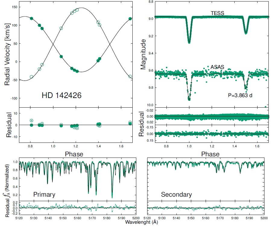
Fig. 1 Radial velocity (left) and light curves (right) of HD142426. The best-fitting models are plotted with black lines. Filled circles on the radial velocity plot refer to high resolution data for the primary, and open ones for the secondary component. On both sides the phase zero is set for the deeper eclipse mid-time, according to the definition in JKTABSDIM. The color figure can be viewed online.
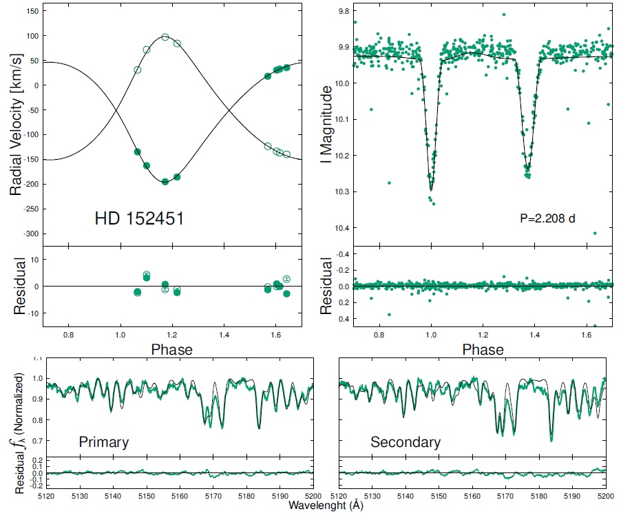
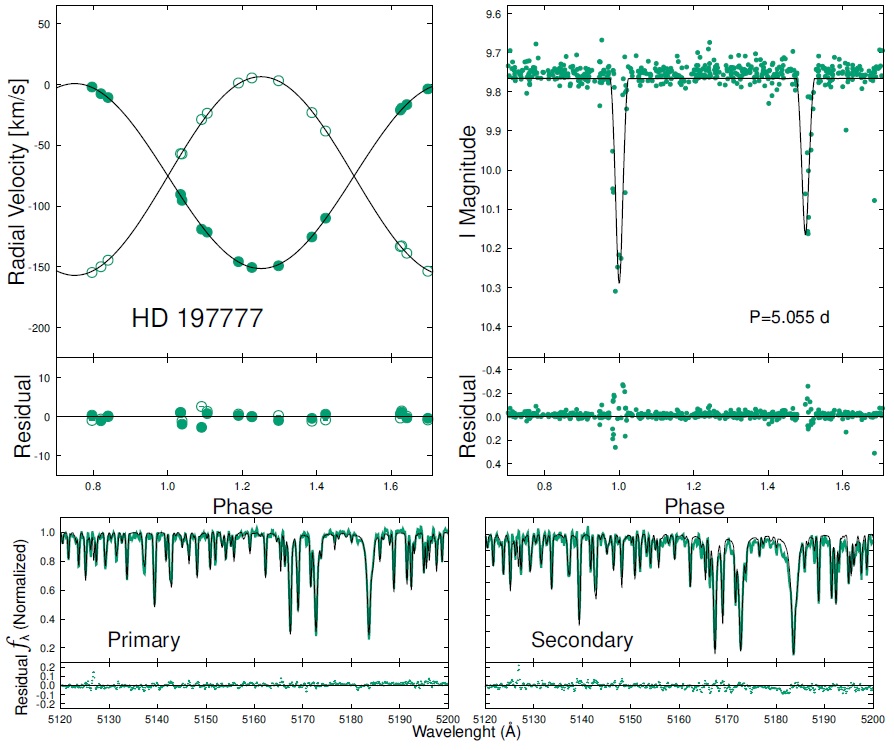
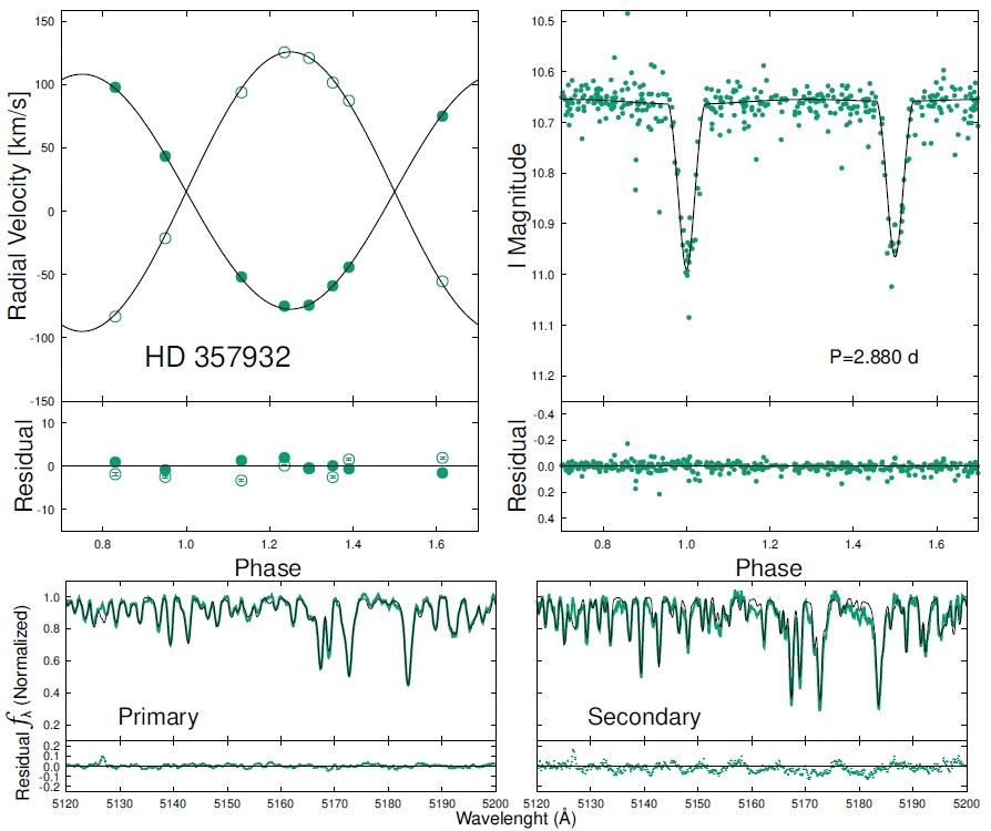
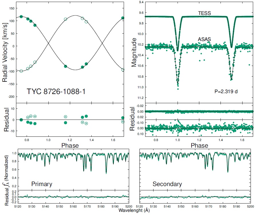
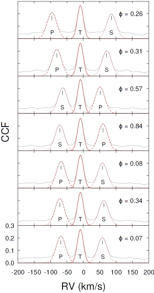
Fig. 6 Sample of cross correlation functions (CCFs) between CD-30 12958 and template spectra at different phases. The Gaussian fits to the two peaks are displayed with a dotted line for the secondary component (S) and with a dashed line for the primary one (P). Short vertical lines mark the centroid velocity of binary components. The tertiary component is indicated with a T. The color figure can be viewed online.
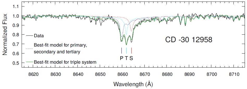
Fig. 7 FEROS spectra of the CD-30 12958 identified as a triple (SB3) system. The three components have different line-of-sight velocities, so many lines can be seen in triple form along the spectra. The SB3 model is overplotted with a good fit. The heliocentric velocity of the tertiary is v helio;3 ≈ 8.8 km s-1 at ᶲ = 0:318 (HJD 56101.6833). The color figure can be viewed online.
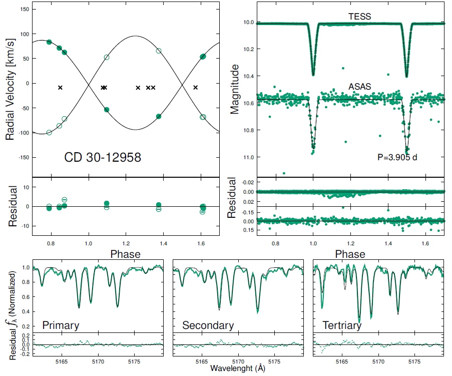
Fig. 8 Radial velocity (left) and light curves (right) of CD-30 12958. The best-fitting models are plotted with black lines. The filled circles on the radial velocity plot refer to high resolution data for the primary, the open ones for the secondary component, and the cross for the tertiary. On both sides phase zero is set for the deeper eclipse mid-time, according to the definition in JKTEBOP. The color figure can be viewed online.
3.2. Light Curve Modelling
Mass, luminosity, and radius are fundamental parameters of any star. In order to determine fundamental parameters, we applied a global fitting of both the photometric data (TESS and ASAS) and radial velocities. This was performed using the JKTEBOP (v40: improvements to the calculation of proximity effects, Southworth, Maxted, & Smalley 2004), which is combined with the Monte Carlo sampler to find the best-fitting model. We note that this software is appropriate for detached EBs where tidal distortion is negligible. It is based on the EBOP code (Popper & Etzel 1981) originally written by Paul Etzel and based on the model of Nelson & Davis (1972). It is a quick procedure that analyses photometric data one set at a time, and in the version used for this paper did not allow for spots or pulsations. Prior to modelling, raw light curves were normalised by their median out-of-eclipse flux based on the ephemerides. Following this step, the final values of the orbital period P, inclination i, eccentricity e, longitude of periastron ω, surface brightness ratio J, and fractional radii of the components r 1,2 were calculated. For systems with several band light curves available (e.g. from ASAS and TESS) the dataset of better quality was used to determine the values of light curve-dependent parameters and to estimate their errors. For each light curve observed with each band, a ’synthetic’ light curve was constructed by evaluating the best-fitting model at the phases of observation. As formal errors are under- estimated, 10 000 iterations of a Monte Carlo algorithm were used to collect statistics on the parameters and yield the final errors.
During the synthesis, the gravitational darkening coefficients were set to β = 0.32 (Lucy 1967) and the limb darkening was modelled with the quadratic law of Kopal (1950) with coefficients taken from van Hamme (1993) and Claret (2017). For the systems in our samples, the third light (l 3) adjustment was not needed to obtain the convergence in most cases. For all systems, reasonable solutions were found assuming l 3=0. However, in the case of CD −30 12958 we expect that some amount of third light is present in the system. CD −30 12958 was a previously unknown eclipsing binary, and the presence of a third companion star was inferred from high-resolution spectra exhibiting signatures of strong third-body lines. The existence of a third-body in the system is explained in the following section.
3.3. Spectroscopic Light Ratio
Since some binary systems are detached, they are good laboratories to derive their light contribution to composite spectra. Detached eclipsing binary stars also pro- vide a robust one-step light ratio determination from their light curves. However, in eclipsing binaries with a partial eclipse, a strong degeneracy generally exists between the radii of the primary and secondary components; numerous light curve solutions exist having different radii r 1 and r 2 but a similar sum of their radii (Graczyk 2003). The degeneracy is breakable if we use proximity effects visible in the light curve. However, detached eclipsing double-lined spectroscopic binaries play pivotal roles in utilizing additional information obtained from the composite spectra of the systems, called the spectroscopic light ratio. The only non-trivial step is the need to determine the ratio of the absorption line strengths for the components. The measured value is a direct indicator of the exact light ratio of the components: a brighter component more strongly dilutes the lines of the fainter companion star and thus the lines of the primary appears deeper and stronger. Inspired by the work of Graczyk et al. (2018), we used the line intensity ratio of the increasing equivalent widths (EW) of metallic absorption lines with decreasing temperature for given chemical composition for the individual components.
Following the method of Graczyk et al. (2018), we first measured the line intensity ratio of the equivalent widths from the strength of the broadening function profiles by using a properly matched template spectrum in RAVESPAN over the wavelength regions 5000 - 6000 Å (ASAS; V- band) and 7000 - 9000 Å (TESS; TESS-band) using the advantage of the large wavelength and spectral stability that FEROS spectra offer, which makes them suitable for detecting narrow absorption features in a wide variety of spectral lines. The templates were calculated from a synthetic spectra library for the temperature and surface gravity of the components. The line intensity ratios I 2/I 1 are given in Table 3.
In order to convert I 2/I 1 into light ratios, we calculated the corrections k 21 following the method of Graczyk et al. (2018). The final spectroscopic light ratios corresponding to the true V-band and TESS-band light ratios were computed simply as the product k 21×(I 2/I 1), and these are also given in Table 3.
3.4. Atmospheric Parameters From Disentangled Spectra
Taking the findings above into consideration, and with an average of ten FEROS spectra for each target well distributed in the orbital phase, it was considered beneficial to carry out a spectral disentangling attempt. This way, we would understand the nature of the binaries and conduct a detailed spectroscopic analysis. We planned to determine the fundamental atmospheric parameters, abundances -which we would need in order to investigate the evolutionary status of the components- and the projected rotational velocity (v sin i) values of the component stars of the systems. For the purpose of spectroscopic identification of the component spectra, spectral disentangling was performed on the time-series of the FEROS spectra, since only these spectra cover the complete optical spectral region on which the determination of the effective temperatures is based.
We used FDBINARY code4 which performs spectral disentangling (Simon & Sturm 1994) formulated in the Fourier space according to the prescription of Hadrava (1995). The fundamental idea implemented in the code is that the most natural way to handle spectra for radial velocity measurements is to express them as a function of x = ln λ instead of as a function of λ (Hensberge, Ilijić, & Torres 2008).
The code is also capable of three-component disentangling, as well as light ratio variations by phase. As we have explained in § 3.3, the only basis in this study is the calculation of light ratio changes of the two components with respect to the orbital phase. The application of the procedure bypasses the step of radial velocity determination, but simultaneously optimizes orbital elements of the system and individual spectra of the binary components instead.
In the runs, we employed the disentangling of several (typically 2 or 3) spectral regions where the contributions from both binary components were clearly visible and we determined orbital elements from each of the considered regions separately. Among the several spectral regions, we focused on the spectral interval of 5 100 - 5 200 Å be- cause it has been well-known for a long time that strong lines with marked wings can be useful tracers of the log g parameter (Gray 2005). We also did some trials to get robust effective temperatures and projected rotational velocities of the components. To get temperatures and projected velocities we chose three absorption lines present in their spectra; Fe I λ4046, Fe I λ4271, and Fe I λ4383. These lines are useful temperature indicators for the dwarf stars as noted in the Gray & Corbally (2009). We also used the initial input parameters (the epoch T 0, the orbital period P, the eccentricity e, the longitude of periastron ω and semi-amplitudes K 1,2) calculated from our orbital solution and light curve modelling in previous sections. The subscripts 1 and 2 denote the primary and secondary components, respectively. Then we applied the disentangling technique to the selected spectral regions to obtain the pure spectrum of each star to be used for the atmospheric analysis.
The resulting disentangled spectra of the primary and secondary components are plotted in Figures 1-5 and Figures 8. After the disentangled spectra of each spectral part were obtained, they were re-normalised considering the average light ratio of components obtained from the initial light curve analysis and the measured light contributions over spectral lines. In this process, the procedure given by Ilijić (2004) was used.
In order to corroborate the estimation of stellar parameters given in Table 4, we used the freely available, Python-based code ISPEC (the Integrated SPECtroscopic framework, Blanco-Cuaresma et al. 2014) to verify the primary and secondary stellar parameters. To maintain the atmospheric parameters we used the spectral synthesis approach, where the key drivers employ the code spectrum (Gray & Corbally 1994), the MARCS grid of model atmospheres (Gustafsson et al. 2008), solar abundances from Grevesse, Asplund, & Sauval (2007), and the atomic line list provided by the third version of the Vienna Atomic Line Database (VALD3, Ryabchikova et al. 2015). ISPEC synthesizes spectra only in certain, user-defined ranges, called ’segments’ which play an integral role in the analysis and are defined as regions of 100 Å around a certain line. We run the fit with the following parameters set free: effective temperature T eff, gravity log g, metallicity [M/H], and rotational velocity v sin i using a set of spectra spread over the orbital period at known times. The resolution R was always fixed to 47 000. The lines are quite narrow, so macro- and microturbulence velocities v mic , v mac were automatically calculated by ISPEC from an empirical relation found by Sheminova (2019) and incorporated into the ISPEC program.
The full optimised parameters are listed in Table 4. The result of an application of this disentangling procedure is illustrated in Figures 1-5 and Figure 8 for the 5 150 - 5 200 Å region. The figures show separated spectra obtained by the disentangling code, and fitted synthetic spectra of the primary and secondary components.
3.5. Physical Properties and Distance
Before discussing the comparison of the model predictions with observational data, we derived orbital and stellar parameters for all the studied systems. Not all systems have their parameters available in the literature. Therefore, we decided to analyse all of them in a uniform way, using photometric and spectroscopic results from the above sections. This was done using the JKTABSDIM code (Southworth, Maxted, & Smalley 2005), which propagates uncertainties via a perturbation analysis. In order to compute by code the absolute parameters of the systems, the necessary input parameters are orbital period (P), eccentricity (e), fractional radii (r 1,2), velocity semi-amplitudes (K 1,2) and inclination (i) (all with formal uncertainties), and the code returns absolute values of masses and radii (in solar units), log(g) and rotational velocities, assuming tidal locking and synchronization. JKTABSDIM can also estimate the distance to the targets, using the effective temperatures of two components, the measured metallicity, E(B − V ) and the apparent magnitudes via various calibrations. The analysis results and their errors are given in Table 4. These resulting parameters were used to place the components on the HR diagrams (Figure 10) for the purpose of examining their evolutionary status.
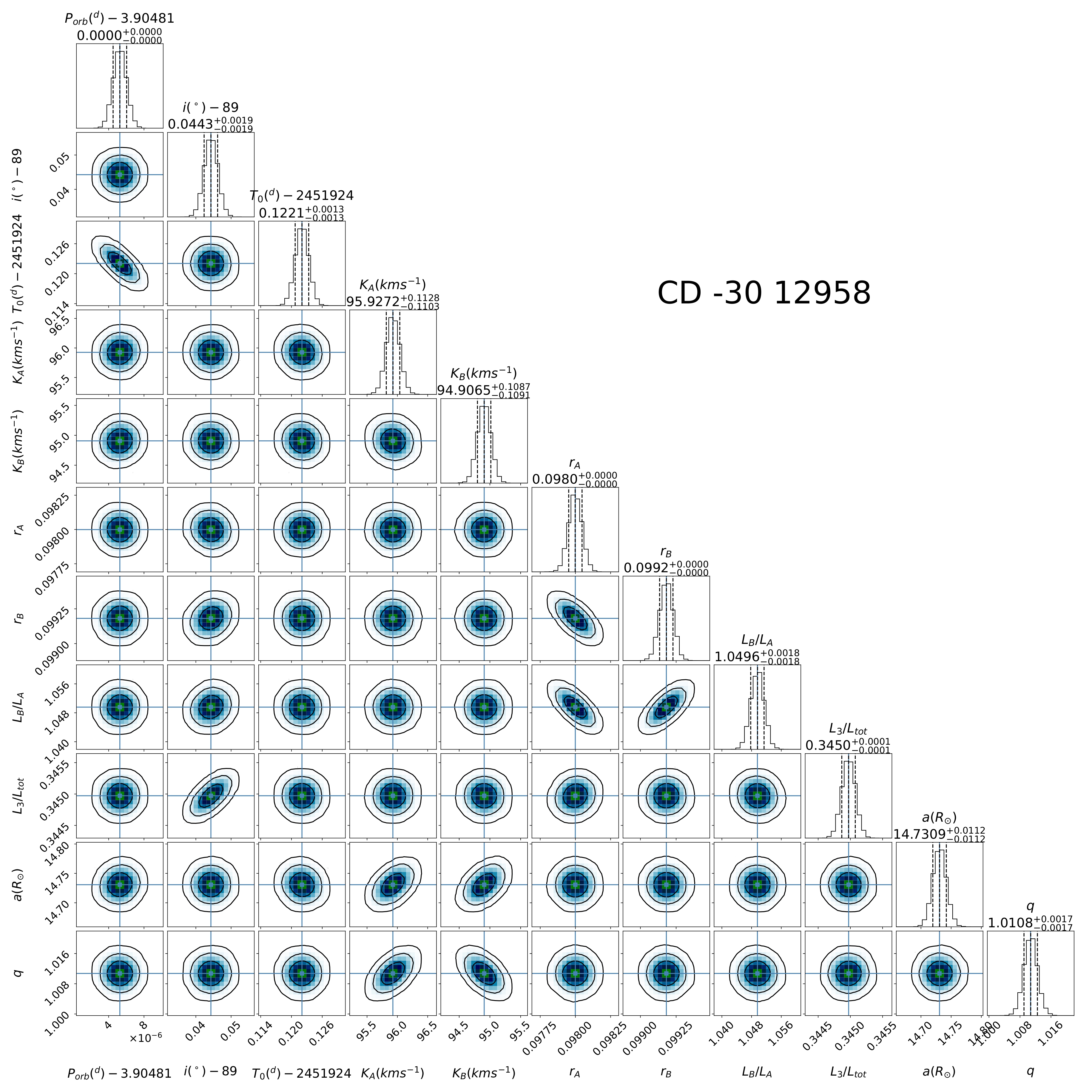
Fig. 9 "Corner plot" (Foreman-Mackey (2016); source code available at https://github.com/dfm/corner.py) for CD-30 12958, illustrating the correlations among the main fit parameters of our solution. Contour levels correspond to 1, 2, and 3σ, and the histograms on the diagonal represent the posterior distribution for each parameter, with the mode and internal 68% confidence levels indicated. More realistic errors are discussed in the text. The color figure can be viewed online.
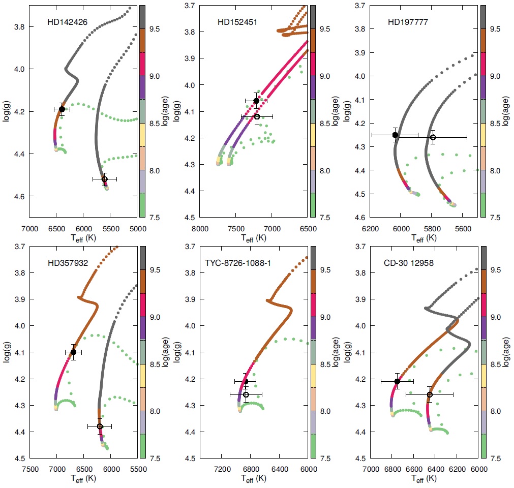
Fig. 10 Comparison of our results with MESA evolution tracks on Teff/log g planes. Primaries are shown with filled circle symbols, and secondaries with open circle symbols, both with error bars from Table 4. The colored points are the evolutionary tracks that best match the calculated component masses, and the colors indicate the stellar age with the color bars at the right side of the plots. The color figure can be viewed online.
The distance to the systems is also straightforwardly measurable. For this, our favored method is via correlation of the reddening to the total equivalent width of the Na I and K I features.
The matter between the stars -the interstellar medium- manifests itself in unforeseen ways, and, as the detritus of stars, its fundamental properties and behavior hold clues to the history and future evolution of stars. Moreover, stars at large distances have been known to show peculiar absorption bands in their spectral analysis. These structures cannot be attributed to stellar lines because they do not follow the Doppler shift caused by the radial motion of the binary components (Merrill 1936). Today, one of best-known absorption features are the Na I (D2 at 5889.951 Å, D1 at 5895.924 Å) and K I (at 7699 Å) lines which are the most noticeable proxies for dust reddening, E(B − V ) (Munari & Zwitter 1997). As we know from the observations, the measurement of reddening value is an important milestone to determine the absolute temperature scale (and therefore the distance) of eclipsing binaries.
Munari & Zwitter (1997) empirically showed some evidence that the Na I D features are unique for tracing reddening for optically thin gas, but saturate for optically thick gas. In our study, we employed the method involved in the empirical relationship found by Munari & Zwitter (1997), which correlates reddening to the total equivalent width of the Na I D absorption lines. The equivalent width was accurately measured simultaneously with several best quality spectra at quadratures, where lines from both components are un-blended with the interstellar ones. The final value of E(B − V ) was then calculated as a sum of the reddenings of individual components of each system. The results for all our investigated binaries are shown in Table 4.
As an independent check on the reddening E(B − V ) we also measured the equivalent width of the interstellar K I (at 7699 Å) line in spectra in which the feature is well resolved from the stellar components. The strength of this line has been found to also correlate with the amount of extinction (Munari & Zwitter 1997), albeit with considerable scatter. Based on a mean equivalent width and on the calibration from the above authors we infer a value of E(B − V ), consistent with the results of Na I lines. The average values are given in Table 4.
Our samples are close neighbours of the Sun, with distances up to 376 pc, and are known as eclipsing binaries. To check the consistency of our estimated distances, we compared our values with the distances obtained from Bailer-Jones et al. (2018, 2021), which are calculated by using Gaia DR2 (Data Release 2; Gaia Collaboration et al. 2016, 2018) and eDR3 (early Data Release 3; Gaia Collaboration et al. 2021) parallaxes. All targets, except CD −30 12958, have accurate parallax measurements in Gaia eDR3. As shown in Table 4, all our calculated distances are compatible with Gaia distances. For the case of CD −30 12958, there is only the Gaia DR2 parallax measurement available and it is not reliable, due to very high uncertainties (≈70 %). Therefore our calculated distance for this target is more uncertain.
The reddening E(B − V ) values we derive from the optical spectroscopy are slightly higher than the predicted reddening from the Schlafly & Finkbeiner (2011) all-sky map. This discrepancy is due to the stars being in different galactic embedded regions. In the next section we will present a brief description of the systems due to their unusual features.
4. RESULTS
In this section, we focus on the results of the combined photometric and spectroscopic analysis of six double-lined eclipsing binaries, and a more extensive discussion of individual systems. Here we also present a brief description of CD −30 12958, which is the close pair in a triple-lined hierarchical system.
4.1. HD 142426
This system was relatively easy to model thanks to high quality photometric and spectroscopic data. First, we used the TESS light curve, which offers very good coverage in eclipses, and sufficient coverage out of them. With no third light contribution and no out-of-eclipse variation, we were able to derive a complete set of orbital and physical parameters, which are given in Table 4. We also analysed photometric data from the ASAS-3 archive (249 observations; a time base of ≈3300 d). HD 142426 turned out to be a double-lined binary (SB2), so we analysed a total of 10 FEROS spectra to cover the binary orbit. We checked the corresponding sky region of HD 142426 using the ALADIN interactive sky atlas (Bonnarel et al. 2000); no source sufficiently bright to affect the ASAS and TESS measurement is situated near our target.
4.2. HD 152451
HD 152451 is the most eccentric eclipsing binary in our sample. It has previously been identified as an eccentric binary with a period of 2.2076 d from the ASAS photometric data (Shivvers, Bloom, & Richards 2014). For the preliminary light curve analysis we used the ASAS V -band photometry, which contained 619 data points. We have also acquired 8 FEROS spectra, and using these, we derived the orbital parameters and the eccentricity of the system. Despite the small number of radial velocity and light curve measurements, the eccentricity precision is significantly better than that of Shivvers, Bloom, & Richards (2014).
The two effective temperatures derived from disentangled spectra were used in JKTABSDIM to calculate the distance. The result, 273(9) pc, is in reasonable agreement with the
The set of parameters given in Table 4 for HD 152451, their precision, and the fact that this system consists of a pair of “twins”, make this target valuable for testing stellar formation and evolution models.
4.3. HD 197777
HD 197777 was initially classified as spectral type F1 in the Henry Draper Catalogue (Cannon & Pickering 1919).
The system was first noted as a double-lined spectroscopic binary in this study and was discovered to be an eclipsing binary by Pojmanski (2002) from ASAS photometry. This system has been observed with FEROS fifteen times, which makes it the most observed target in our sample (spectroscopically). We obtained the light curve of the system from the ASAS catalog and with a deeper primary minimum by folding with the orbital period given.
HD 197777 consists of two solar-mass stars of significant age (age > 9 Gyr) with nearly equal masses and radii. The inferred distance for the system is compared with the Gaia eDR3 results in Table 4. The estimated distance is in relatively good agreement with Gaia eDR3.
4.4. HD 357932
HD 357932 was initially classified as spectral type F0 in The Henry Draper Extension Charts (HDEC) (Nesterov et al. 1995); published in the form of finding charts, it contains spectral classifications for some 87 000 stars mostly between 10 th and 11 th magnitude. These data, while highly valuable, were unfortunately practically useless for modern computer-based astronomy.
A binary model for HD 357932 was obtained for the first time, using a combined analysis of ASAS light curve data and high-resolution FEROS spectra. We used an automated procedure to create the model, based on the JKTEBOP binary modelling code. In order to obtain the spectra of the components from the composite FEROS spectra of the system, we used the disentangling method, and we obtained a higher signal-to-noise mean component spectrum for both the primary and the secondary. From the joint fitting of the eclipse photometry, radial velocity analysis results and spectral disentangling results, we determined the masses of the HD 357932 binary with 3 % precision and the radii with 1 %-2 % precision. With such highly precise parameters, we were able to test stellar evolutionary models for solar-type stars, comparing the predictions of such models in the HR diagram.
4.5. TYC 8726-1088-1
TYC 8726-1088-1 is listed by Pojmanski (2002) as an eclipsing binary system with a period of ≈2.819 d. Aside from brightness (apparent V magnitude: 10 m .7) and position measurements (Høg et al. 2000), no literature data are available and no light curve solutions or radial velocity studies have been attempted so far.
Comparison of the JKTABSDIM output showed that the two components of the system are indistinguishable, and as a result absolute parameters differ typically by 1-3 % of the obtained errors. We therefore adopted the derived results as the final ones and we accepted the system as a twin binary (mass ratio q ≃ 1); such systems are exceptional tools to provide information for probing the internal structure of stars.
For the distance determination, we adopted the interstellar reddening of E(B − V ) as derived from the correlation reddening of the total equivalent width of the Na I D absorption lines. The distance calculated with the trigonometric parallax from the Gaia eDR3 is about 90 % of the value found in our calculations.
TESS, ASAS I-band light curve, and radial velocity curve for the system are presented in Figure 5. Using our new precise analysis we classified the system as F3 type for the first time.
4.6. CD −30 12958
CD −30 12958 is the second longest-period system in this study. This star is listed in the ASAS-3 Catalogue (565 observations; a time base of ≈3200 d). Eclipse variations in the system light curves are noticeable. Except for the brightness (apparent V magnitude: 10 m .5) and position measurements (Høg et al. 2000), no literature data are available and no light curve solutions or radial velocity studies have been attempted so far.
High-resolution spectra revealed that CD −30 12958 is likely a hierarchical triple, with the eclipsing binary components in a non-eccentric orbit and a third light contribution of over 30 %.
The eclipsing binary is composed of F5-type stars with masses: M p = 1.36(3) M ʘ and M s = 1.24(3) M ʘ, and radii: R p = 1.49(1) R ʘ and R s = 1.36(2) R ʘ. The third component has a similar spectral type (F3V) and is on a wide orbit. Its contribution to the total light from the light curve analysis is about 34 %, which is consistent with the value derived from spectral disentangling (35 %).
In the high-resolution FEROS optical spectra, CD −30 12958 appeared as triple-lined. The nearly equal peaks on the cross-correlation function (CCF) corresponding to the primary and secondary components are the strongest in this system, followed by a tertiary corresponding to a slightly weaker one (Figure 6 and 7). We measured the radial velocity of all components, denoted as a black cross in Figure 8, with the primary (filled circle) and the secondary (open circle) stars.
In order to calculate the random errors of the initial values of parameters (including l
3), we used the Monte Carlo simulation algorithm implemented in JKTEBOP , which was found to quantify the correlations between the parameters. For each ASAS I-band and TESS light curve, a ‘synthetic’ light curve was constructed by evaluating the best-fitting model at the phases of observation. This process was undertaken 10 000 times for each observed light curve of the system. The standard deviation of the distribution of values for each parameter has been calculated. A sample plot of the distributions of different parameter values for CD −30 12958 is shown in Figure 9. From the predicted temperatures for the primary and secondary, we determined the distance as 290(13) pc with the E(B − V ) value derived from Na I D1 given in Table 4. The resulting distance is inconsistent with the Gaia DR2 value of
5. AGE AND EVOLUTIONARY STATUS
The accurate stellar fundamental parameters that can be derived from eclipsing binaries offer opportunities to confront our current stellar structure and evolution theories with observations.
In Figure 10, we show a comparison of the results of our analyses with theoretical MESA evolution tracks developed as part of the MESA Isochrones and Stellar Tracks project (MIST5 v1.2, Dotter 2016; Choi et al. 2016). For each system, we determine the age at which the observed or calculated properties of both components are best represented. Because the stellar temperature T eff is one of the most robust resulting parameters from the spectral analysis we compare our data on T eff/log g planes. One important caveat is that the measured T eff values of the components are independent.
We located each component in the systems using the T eff and log g determined by the JKTABSDIM code and compared them with the MESA tracks corresponding to the masses derived from the spectro-photometric analysis. This procedure allows us to infer the ages of each component in the binary systems. Each pair resulted to be nearly coeval, except for CD −30 12958. The ages of its components do not show agreement with each other. This may be caused by the contamination of the third component in the spectral disentangling procedure, which could affect the light curve modelling or radial velocity measurement.
6. SUMMARY AND CONCLUSIONS
In this study, we present physical parameters of six targets from our investigation, with the aim of characterizing interesting eclipsing binary systems by taking into account all available data. The orbital and physical parameters of the stars are shown in Table 4. The errors of the parameters, also given in Table 4, are calculated with the JKTABSDIM procedure using the parameters and uncertainties from the radial velocity and light curve analysis described above.
High quality photometric (TESS + ASAS) and spectroscopic data (FEROS) allow us to obtain the masses and radii of the components with a precision better than 3 % for the systems, making them reliable test-beds for accurately understanding the origin and evolution of binaries.
We also emphasise that precise fundamental and orbital parameters of solar analogue type stars are vital for exoplanet studies (Allard, Homeier, & Freytag 2012; Huber et al. 2014; Johnson et al. 2007). Since the fundamental planet parameters are tightly bound to the host star properties, spectroscopic or photometric orbit solutions and estimation of fundamental parameters of the stars should be obtained with a precision better than 3 %, which we achieve in this study. For this reason, this study is also important to determine the fundamental parameters of candidate super Earth-mass planets that will be discovered as a result of ongoing observations of TESS.
One of the objects, CD −30 12958, shows lines coming from three components in its spectra. Further work on the object should focus on eclipse time variation analysis in order to independently determine orbital and physical parameters.

