


 nova página do texto(beta)
 Inglês (pdf)
 Artigo em XML
 Referências do artigo
 Enviar este artigo por email
 Citado por SciELO
  Similares em
SciELO
Similares em
SciELO 
 Permalink
1. INTRODUCTION
In their article on BL Cam and DY Peg, two SX Phe stars, Blake et al. (2000) reported that Hintz et al. (1997) on studying the rate of period change for BL Cam found that over an observational baseline of 30 years, BL Cam had exhibited a steady period change with no sudden jumps. However, they found that the light curve of BL Cam was exhibiting periodic amplitude variations of up to 0.2 magnitude. Such behavior was unexpected and had not been previously reported.
The most recent study of BL Cam (= 2MASS J03471987+6322422, Gaia DR2 487276688415703040, GD 428 in Simbad) is that of Zong et al. (2019) with observations from 2014 to 2018. They determined that the period content of BL Cam was dominated by a frequency of 25.5790 (3) c/d and its two harmonics, plus an independent frequency of 25.247 (2) c/d, a non-radial mode frequency detected from the data in 2014. With a O−C analysis of their times of maxima from the literature they determined a periodic change which, if caused by the light-time travel effect (LTTE), made BL Cam a binary system. Besides, they did not find evidence of the triple system suggested by previous authors.
We must remark that despite high quality space missions like TESS and the analysis of their data on A-F stars (Antoci et al. 2019), observational programs that have enough time series data to study the rate of period change must be developed, which is a task not possible to perform with TESS observations.
The Observatorio Astronómico Nacional de Tonantzintla (TNT) finds itself in an analogous situation to that described by Blake et al. (2000) referring to York University Observatory, since they are both located near large metropolitan areas. This restricts the types of research projects that can be conducted to those not requiring absolute photometry. Given the occasional large gaps in observational coverage of HADS and SX Phoenicis stars that have hindered the study of their period changes for several years, we have carried out a long-term monitoring program for such variables. Here we report our observations of BL Cam obtained as part of this program conducted by the staff and students of the Observational Astronomy courses of the National University of Mexico at TNT. These observations have been supported with uvby − β photometry from the Observatorio Astronómico Nacional de San Pedro Mártir (SPM), México.
The purpose the present paper is to describe the procedure to acquire the new times of maximum, observations and reduction. With the new times of maximum and those found in the literature we analyzed them with an O-C procedure. The residuals derived utilizing the ephemerides values of Zhou et al. (1999) are congruent with a physical explanation, and suggested a periodic function, so we analyzed them with Period04. This package provided the orbital parameters assuming a binary system. The physical parameters are determined from uvby − β photoelectric photometry and the unreddening procedure of Nissen (1988). The unreddened values were compared with the grids of Castelli & Kurucz (2006).
A brief summary of the contents of each section is the following: a description of the observations and data reduction is presented; period determination was done by the O−C procedure studying the proposed ephemerides. Our conclusion is that the star behaviour is explained if we assume a binary system, and so we determined the orbital elements and mass of the companion star; to conclude, we determined from uvby −β photometry, its metallicity, surface gravity and effective temperature.
2. OBSERVATIONS AND DATA REDUCTION
Although some of the times of maximum light of this star have been reported elsewhere (Peña et al., 2021), here we present new times of maxima and the procedure followed to acquire the data. The observations were done at both the Observatorio Astronómico Nacional of San Pedro Mártir and Tonantzintla, in México. Table 1 presents the log of observations, as well as the new times of maximum light.
TABLE 1 LOG OF OBSERVING SEASONS AND NEW TIMES OF MAXIMA OF BL CAM
| Date | Observers/Reductors | Npoints | Time span | Nmax | Tmax (HJD-2458000) | Observatory |
|---|---|---|---|---|---|---|
| yr/month/day | day | day | ||||
| 20/01/1112 | hh,ESAOBELA20/hh,jdp | 122 | 0.0960 | 3 | 860.7052 | TNT |
| 860.7448 | ||||||
| 860.7842 | ||||||
| 20/01/1213 | hh,ESAOBELA20/hh,jdp | 162 | 0.1396 | 3 | 861.7247 | TNT |
| 861.7641 | ||||||
| 861.8022 | ||||||
| 20/01/1314 | hh,ESAOBELA20/hh,jdp | 116 | 0.0880 | 3 | 862.7415 | TNT |
| 862.7804 | ||||||
| 862.8204 | ||||||
| 20/01/1415 | hh,ESAOBELA20/hh,jdp | 151 | 0.1230 | 3 | 863.7182 | TNT |
| 863.7599 | ||||||
| 863.7959 | ||||||
| 20/01/1617 | hh,ESAOBELA20/hh,jdp | 117 | 0.0906 | 2 | 865.7510 | TNT |
| 865.7905 | ||||||
| 20/01/1718 | hh,ESAOBELA20/hh,jdp | 146 | 0.1187 | 2 | 866.7287 | TNT |
| 866.7684 | ||||||
| 20/02/2425 | dsp/dsp,jdp | 40 | 0.0819 | 2 | 904.6927 | SPM |
| 904.7318 | ||||||
Notes: dsp, Piña D. S.; hh, Huepa H.; jdp Paredes, J. D.; ESAOBELA20: Carrasco, L.; Vargas, C., Martínez, G., Castellanos, M., Mejía, N., Buenfil, G., Vásquez, F., Martínez, B., León, A., Beato, M. & Paredes, J. D.
A 10-inch Meade telescope equipped with an Andor Apogy CCD camera was utilized at the TNT Observatory. There were around 11,000 counts with an integration time of 1 min, enough to secure high precision. The reduction work was done with AstroImageJ (Collins & Kielkopf 2013) Period determination. This software is relatively easy to use and besides being free, it works satisfactorily on the most common computing platforms. For the CCD photometry two reference stars were utilized in a differential photometry mode. The results were obtained from the difference Vvariable−Vreference and the scatter was calculated from the difference Vreference1 − Vreference2. Light curves were also obtained. The new times of maximum light are listed in Table 1.
3. O−C ANALYSIS
3.1. O−C
Before calculating the coefficients of the ephemeris equation, we studied the existing literature related to BL Cam. Several authors have carried out studies of the O−C behavior of this particular object and developed models. When these models were constructed, they were built with the data available to them based on the length of their observation time. However, they often differ in the interpretation of the data.
Hintz et al. (1997) presented a thorough study of this star concluding that BL Cam is a double-mode variable with a primary period of 0.0391 day, with evidence that the fundamental period had increased by 0.009 s in the previous 20 years. Their determined variation differs from that of McNamara and Feltz (1978) who proposed a linear variation. They found that the best fit to the data was given by equation (1), and concluded that the period had changed by 0.009 s in the last 20 years:
It was Hintz et al. (1997) who decided that this star had an increasing period and Blake et al. (2000) corroborated this assertion. Using their observations those authors proposed that the amplitude of the star’s light curve is modulated and that the physical cause may be tied to the fact that the star is known to exhibit the features of double-mode pulsation. However, works such as Wolf et al. (2002) could not confirm the results of Hintz et al. (2000) implying that the star had a constant increasing pulsational period. Their conclusion, as expected, was that this star deserved continuous monitoring. One year later Kim et al. (2003) found that the parabolic period variation had recently reversed.
In view of the discrepancies among the different authors, we did a follow-up of the literature that contained ephemerides equations with the data available at that epoch. Most of the ephemerides equations have been calculated utilizing equation 2, in which P is the period, in days; β is the rate of the variation; Z, is the zero point; B is the amplitude; Ω, the frequency and α, the phase. These ephemerides elements are presented in Table 2.
with
TABLE 2 COMPILATION OF THE LITERATURE
|
|
Period (day) | A |
|
|
|---|---|---|---|---|
| Berg77 | 2,443,125.80476 | 0.0390883 | ||
| McNamara78 | 2,443,125.8048 | 0.03909760 | 0.0011 | |
| Hintz97 | 2,443,125.8042 | 0.03909773 | 6.153 |
0.00068 |
| Zhou99 | 2,443,125.8041 | 0.03909771 | 3.5728 |
0.0013 |
| Conidis13 | 2,443,125.8026 | 0.039097911 | 2.86 |
0.0045 |
| Zong19 | 2,443,125.7748 | 0.0390980385 | -2 |
0.0015 |
Notes. Berg77: Berg & Duther (1977); McNamara78: McNamara & Feltz (1978); Hintz97: Hintz et al. (1997); Zhou99: Zhou et al. (1999); Conidis13: Conidis & Delaney (2013); Zong19: Zong et al. (2019).
Notes: Compilation of the literature that presented ephemerides equations with the data available during their analysis.
In Table 3, we list the author and the year of publication in Column one, Columns two and three show the initial and final dates of the data they analyzed, Column four shows the time span they considered, in years; the next column shows the number of points in their analysis consisting of the points they obtained combined with those of the literature at that time; the last column lists the number of points each author observed. The behavior/ of their O−C analysis is shown schematically in Figure 1.
TABLE 3 CHRONOLOGY OF THE COMPILATION
| References | (HJD - 2400000) |
(HJD - 2400000) |
|
N( |
N(observed) |
|---|---|---|---|---|---|
| Hintz97 | 43125.8046 | 50151.7268 | 19 | 69 | 39 |
| Zhou99 | 43125.8046 | 50447.1520 | 20 | 136 | 58 |
| Kim03 | 43125.8046 | 52272.1994 | 25 | 249 | 104 |
| Fauvaud06 | 43125.8046 | 53478.4921 | 28 | 415 | 105 |
| Conidis13 | 43125.8046 | 55635.6073 | 34 | 1465 | 73 |
| Zong19 | 43125.8046 | 58413.3119 | 41 | 1583 | 123 |
Notes: Chronology of the compilation of times of maximum by several authors. The time span and number of points in the database employed in the literature are presented.
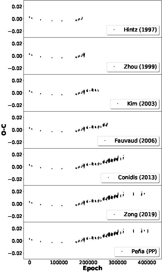
Fig. 1 O−C diagrams calculated with data from different authors (see main text) employing the ephemeris given by Zhou et al. 1999.
For our analysis we collected a total of 520 times of maximum light from the literature and our observations. To these data we added those of VizieR to get 1985 data points, some of which were duplicated. Removing these repeated values, we got a total of 1606 data points. The elapsed time of observations is from 2443125.8046 to 2458904.7320 for a time span of 15778 days, or forty-three years, a considerable length of time.
The starting point for our O−C analysis was that provided by Zhou et al. (1999), who utilized the
ephemerides listed in equation 1 proposed by McNamara et al.(1978). As a first stage, we reproduced what Zhou et al. (1999) obtained in their O−C
residuals with their 136 times of maximum light, in which we can see that the
parabolic behavior interpretation was logically inferred (see Figure 2). It is important to mention that
they report a change in rate of

Fig. 2 Behaviour of the data points of Zhou et al. (1999) calculated reproducing their results: Top, the logically inferred parabolic behavior interpretation. Bottom, the O-C residuals calculated both linearly and quadratically. The plots use their own time span.
We have extended the time basis with the new values of
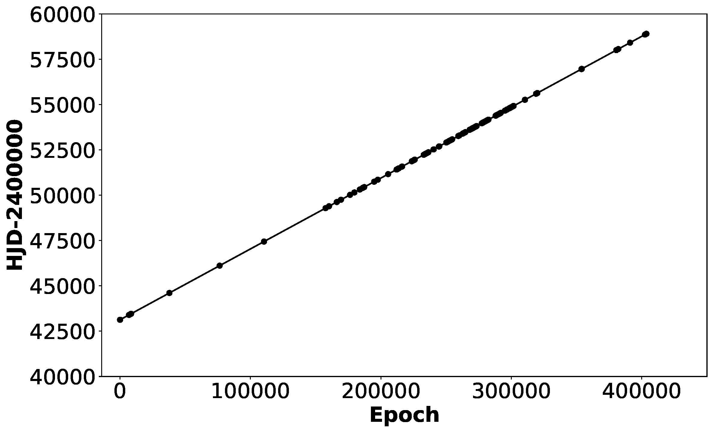
Fig. 3 Graphic representation of the linear equation 3 originally calculated by Zhou et al. (1999) that includes the new ephemerides elements with an extended time basis of 23 years. The new determined values are T 0 = 2443125.7938(2) d and P = 0.0390979132(9) d/cycle.
With these new determined values we calculated the new O−C values represented in Figure 4, analogous to those presented by Zong et al. (2019) in their Figure 5.
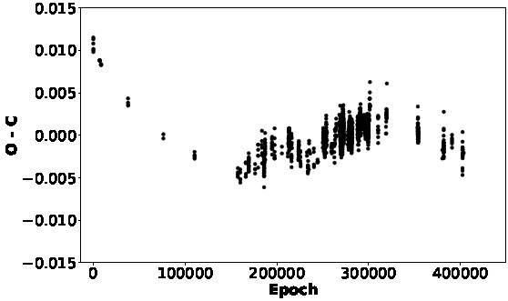
Fig. 4 O−C residuals of the 1606 data points with the new ephemerides equation deduced by a linear fit. This resembles equation 3 in Zong et al. (2019).

Fig. 5 Behavior of the O−C residuals for the whole sample of the 1606 data points with the ephemerides elements listed in equation 2 of Zhou et al. (1999) as a function of cycles. The color figure can be viewed online.
However, they arbitrarily discarded all O−C data points with E less than 150000 cycles because they showed an unexplained behaviour. Given the analogous results we obtained from Zong et al. (2019), we could have proceeded in the same fashion but, we preferred to consider all the O−C elements in the ephemerides procedure in Zhou et al. (1999).
Zong et al. (2019) carried out an exhaustive analysis of the O−C residuals. Their origin was based on the work of Fu et al. (2008) who suggested that the main period of BL Cam might have undergone an abrupt change. This change was studied by Fauvaud et al. (2010) and by Conidis & Delaney (2013) who suggested that the change of the main period might be caused by a third body explained by a cubic curve adjustement shown in their Figure 5, which is presented here in Figure 4.
However, the model proposed by Zhou et al. (1999) shows that the main frequency derived in the O−C analysis is quite consistent with the fundamental frequency decomposed by Fourier transforms which explains all the times of maxima. Following this approach, we utilized Zhou et al.’s (1999) equation and considered the number of cycles and the O−C for the extended time basis all the elements, including those below an E of 150000 which Zong et al. (2019) had discarded. The smooth variation presented in Figure 5 was obtained if a sinusoid was assumed. If we only take the time span employed in Zhou et al (1999) into account, the logical deduction would be a parabolic behavior. This parabolic assumption was also assumed by Fauvaud et al. (2006) although their time basis was not long enough to reach a different conclusion, but when the elapsed time was extended, a sinusoidal variation can be seen.
Due to the fact that a sinusoid can be considered, in Figure 5 we calculated the variation parameters through a fit obtained with Period04, a canonical procedure utilized for short period variable stars (Lenz & Breger, 2005). Period04 is a computer program especially dedicated to the statistical analysis of large astronomical time series containing gaps. The program offers tools to extract the individual frequencies from the multiperiodic content of time series and provides a flexible interface to perform multiple-frequency fits. The Fourier analysis in Period04 is based on a discrete Fourier transform algorithm.
This fit to a sinusoid is shown in the Figure 5 by the continuous line, which explains those points discarded by Zong et al. (2019) and the newly observed points in 2020. The output of Period04 is presented by the following equation 4, with the numerical values presented in Table 4. It is shown schematically in Figure 6.
TABLE 4 COEFFICIENTS DERIVED WITH PERIOD04
| Parameter | Values | Uncertainty |
|---|---|---|
| Ω1 | 178 ×10−8 | 2 ×10⁻⁸ |
| B 1 | 923 ×10−5 | 8 ×10⁻⁵ |
| α 1 | 576 ×10−3 | 2 ×10⁻³ |
| Z | 64 ×10−4 | 1 ×10⁻⁴ |

With an extended time span it becomes evident that the conclusion reached previously was partial because it was obtained based on the limited time span at that time. Now, we postulate a sinusoidal behavior that could be explained by the presence of another unseen companion star and the light travel time effect (LTTE). Due to the above, we adjusted the equation:
to determine the optimized parameters for the equation to get the best fit to the data, we utilized the algorithm of Levenberg-Marquardt. As initial parameters we considered a 0 equal to 2Z and w = 2πΩ1. To the remaining coefficients we assigned zero values. The obtained optimized parameters and their standard deviations are presented in Table 5 for a frequency of w = (122 ± 2) × 10−7 (1/d). This new analysis provides an orbital period of the star with a result of P orb = 55.2 years. This postulation will be tested with continuous monitoring of this star over the next 12 years when the 55.2 years period that we predict will be completed. The results are shown in Figure 7.
TABLE 5 FOURIER COEFFICIENTS
| [Values]×10−4 | [Uncertainty]×10−4 | |
|---|---|---|
| a 0 | 59 | 1 |
| a 1 | -29 | 3 |
| a 2 | -5 | 1 |
| b 1 | -91 | 2 |
| b 2 | -5 | 2 |

Fig. 7 New fit obtained utilizing Fourier series considering equation 5 and the Fourier coefficients listed in Table 5.
Subtracting the calculated fit, we obtained the results presented in Figure 8. No clear evidence of another frequency exists as Fauvaud et al. (2010) and Conidis et al. (2013) proposed, but from our analysis it cannot be discarded due to the lack of observations in the cycle intervals between [0, 142000] and [330000, 382000] which makes the analysis difficult. Calculating the standard deviation of the residuals we get σ = 0.0012, less than that obtained by Zhou et al. (1999), Conidis et al. (2013) and Zong et al. (2019). This supports the sinusoidal behavior shown in the O−C diagram of Figure 7.

Fig. 8 Residuals after the Fourier series fit shown in Figure 7. The central horizontal line represents the mean value and the other extreme lines the standard deviation of the residuals.
3.2. Determination of Orbital Parameters and Mass of the Companion Star
Carrying out an analysis of a binary system such as that developed by Zong et al. (2019), it is possible to determine the parameters of the companion star utilizing the formulae 6, 7 and 8 proposed by Borkovits et al. (1996), which are function of the Fourier coefficients.
where a 0 is shown in equation 5; a 1,2 ; b 1,2 are the Fourier coefficients. These are listed in Table 5. A ’ denotes the semi-major axis. i ,e y w are the elements of the orbit of the companion, c is the speed of light in astronomical units per day.
Then, we followed Borkovits & Heged¨us (1996) for the determination of the mass of the companion star.
Considering a three body system, Borkovits & Heged¨us (1996) present equation 11 in their paper as a solution which we used, adapting it to a binary system in which BL Cam orbits around another unseen star and the encountered variations in the O−C are provoked by the LTTE. This follows a prescription first employed by Fu et al. (2008). Combining them, equation 9 provides the mass function in terms of the orbital parameters.
Substituting the above-mentioned values listed in Table 6 calculated in this work in the mass function equation given in equation 9, it is possible to calculate the mass of the companion. Considering the mass of BL Cam as m 1 = 0.99 from McNamara (1997), we calculated the mass m 2 for different angles i , shown in Table 7, determining the roots of the polynomial given in the equations:
TABLE 6 PARAMETERS OF THE COMPANION STAR OF BL CAM
| Orbital Parameter | Value |
|---|---|
|
|
0.15 |
|
|
281.76 |
|
|
1.65 |
|
|
55.2 |
TABLE 7 MASS OF THE COMPANION AS A FUNCTION OF THE ANGLE
| Angle | Semi-major axis | Mass |
|---|---|---|
| 20 | 4.8 | 0.42 |
| 25 | 3.9 | 0.32 |
| 30 | 3.3 | 0.27 |
| 40 | 2.6 | 0.20 |
| 50 | 2.2 | 0.16 |
| 60 | 1.9 | 0.14 |
| 70 | 1.8 | 0.13 |
| 80 | 1.7 | 0.12 |
Being a cubic equation, it has three solutions. In each case we considered as a solution the real root. The other two are imaginary roots without physical interpretation. The mass of the companion star as a function of the inclination angle is shown in Table 7.
The behavior of mass as a function of angle is shown in Figure 9. Given the obtained values we can say that we are dealing with a M-type star.

3.3. Period Determination Conclusions
Despite having been determined to be a variable star many years ago, the variability of the SX Phe star BL Cam has been described with several interpretations as more information has been gathered. Considering the interpretation of this century only, we highlight the following studies.
Kim et al. (2003) found that the parabolic period variation had recently reversed. They also determined five frequencies for BL Cam using Fourier analysis. They stated that in order to confirm the periodic variation of the O−C values, BL Cam should be observed for at least 10 more years.
Rodriguez et al. (2007) reported that their results confirmed the existence of multi-periodicity in this star. In addition to the main frequency f 0=25.5769 c/d and its harmonics 2f 0 and 3f 0, with stable amplitude, a secondary frequency f 1 exists in the region 31-32 c/d with variable amplitude.
A more recent article, that of Fauvaud et al.
(2010), states that the short-term O−C variation, if interpreted as a
light travel-time effect, is indicative of a massive stellar component (0.46 to
1
Conidis and Delaney (2013) found a more accurate period of 0.039097912(1) days, and presented an updated linear ephemeris. This newly presented linear ephemeris was used to calculate revised O−C values, which were fitted with a parabolic curve to measure the rate of change of the pulsation period.
Although the parabolic fit has a physical interpretation, it is noted that a cubic fit more appropriately describes the behavior of the O−C diagram, but they concluded that this assumes the O−C diagram is best represented by a quadratic fit. This has been shown to be a poor assumption, since a cubic polynomial is a better representation of the O−C diagram. This, according to them, is problematic since the physical meaning of the third order term cannot be explained physically.
The most recent paper, that of Zong et al. (2019) did not find evidence of a triple system as stated by Fu et al. (2008). Fauvaud et al. (2010) performed a triple system analysis of the O−C diagram. However, the determination of the second companion’s parameters was not successful. The residuals of fitting the O−C curve implied that BL Cam might be a binary system in an eccentric orbit with a period of 14.01 (9) yr. The companion might be a brown dwarf.
In this study, with an extended time basis of 15779 days or 403578.6 cycles, we performed an O−C analysis and found that the residuals do not conform to the parabolic variation proposed by other authors but rather present a sinusoidal variation with a period of 60 years.
In our analysis we do not need to invoke multi-periodicity as was previously proposed, nor a parabolic behavior. Instead, with only one stable period, using Period04, we adjusted the 1606 times of maximum light shown in Figure 5. Our final fit is obtained using equation 5 and is presented in Figure 7; its residuals are shown in Figure 8.
Considering the obtained results of the present work, and taking into account the residuals in the σ interval presented in Figure 8, this paper has shed light on the nature of BL Cam. Before we consider that it might be a triple system, as Fauvaud1 (2010) proposed, continuous monitoring of the star is mandatory.
4. PHYSICAL PARAMETERS
In this section, we consider uvby −β photometry to determine some physical parameters. With this photometric system it is possible to determine reddening and unreddened values via the procdure proposed by Nissen (1988). The accuracy of our photometry is evaluated by three methods. From these we determined the metallicity [Fe/H] and by comparing the unreddened indexes c 0 and (b−y)0 with the Castelli & Kurucz (2006) models effective temperature and surface gravity were estimated.
The uvby − β photometric system has the advantage that reddening and unreddened colors can be determined from the photometry and the proper calibrations. One of the pioneer works in this matter was that of Crawford and collaborators. Later, in 1988, Nissen (1988) extended the sample of clusters to thirteen and developed empirical calibrations which determined the intrinsic color index (b − y)0 in terms of the other color indexes and β utilizing as reference the Hyades. Nissen’s (1988) procedure is applicable for A and F type stars. For F type stars (2.59 ≤ β ≤ 2.72) the intrinsic color index (b − y)0 is calculated by the expression:
4.1. Data Acquisition and Reduction at SPM
At the SPM Observatory the observational, as well as the reduction procedures, have been employed since 1986 and have been described many times. A recent detailed description of the methodology can be found in Peña and Martinez (2014).
The star BL Cam was observed in uvby−β photometry in February, 2020. The season covered five nights during which BL Cam was observed on two. Over all the nights of observation the following procedure was used: each measurement consisted of five ten-second integrations of the star and three tensecond integrations of the sky simultaneously for the uvby filters and almost simultaneous for the narrow and wide filters that define Hβ.
The accuracy of our observation was evaluated by three numerical procedures: (i) the accuracy of each point; (ii) a comparison of the observed standard stars with those values in the literature, and (iii) a comparison of the observed standard stars obtained in each night throughout the whole season.
In the first case, the accuracy is a direct result of the star counts. Although BL Cam is a faint star for our telescope-spectrophotometer system we obtained in the five ten-seconds integrations, enough counts to calculate the errors for the u, b, v, and y filters that define the uvby−β photoelectric photometry, equal to (18491, 53040, 68053, 24413), respectively, which translated into uncertainties of (0.0074, 0.0043, 0.0038, 0.0064) magnitudes.
For the second criterion we reduced each night separately calculating the transformation coefficients and the difference in magnitude between the obtained values and the values reported in the literature for each night. To calculate the final photometric values we averaged the nightly coefficients and the differences with the literature. With the obtained photometric values we reduced the data as described in Peña & Martínez (2014). What must be noted here are the transformation coefficients for the observed season (Table 9). This led to the obtainment of the final photometric values. The season errors were evaluated using the observed standard stars with those employed from the literature. These uncertainties were calculated through the differences in magnitude and colors for (V , (b − y), m 1, c 1 and Hβ) which are (0.035, 0.008, 0.011, 0.011, 0.012) for the 2020 season.
TABLE 8 MEAN PHOTOMETRIC VALUES AND STANDARD DEVIATIONS OF THE STANDARD STARS OF THE 2020 SEASON
| ID | V | (b−y) | m 1 | c1 | β | σV | σ(b−y) | σm 1 | σc 1 | σβ | N |
|---|---|---|---|---|---|---|---|---|---|---|---|
| HD114710 | 4.233 | 0.365 | 0.195 | 0.340 | 2.600 | 0.004 | 0.003 | 0.002 | 0.006 | 0.014 | 5 |
| HD111812 | 4.944 | 0.429 | 0.204 | 0.406 | 2.589 | 0.044 | 0.003 | 0.004 | 0.005 | 0.016 | 5 |
| HD28355 | 5.000 | 0.113 | 0.240 | 0.890 | 2.847 | 0.010 | 0.003 | 0.003 | 0.007 | 0.016 | 5 |
| HD69897 | 5.117 | 0.314 | 0.148 | 0.383 | 2.630 | 0.010 | 0.002 | 0.002 | 0.005 | 0.013 | 8 |
| HD115383 | 5.176 | 0.369 | 0.190 | 0.390 | 2.615 | 0.005 | 0.003 | 0.003 | 0.003 | 0.015 | 5 |
| HD154029 | 5.255 | 0.002 | 0.174 | 1.098 | 2.871 | 0.021 | 0.002 | 0.004 | 0.008 | 0.012 | 5 |
| HD157214 | 5.374 | 0.395 | 0.178 | 0.318 | 2.571 | 0.008 | 0.003 | 0.004 | 0.006 | 0.015 | 5 |
| HD76398 | 5.427 | 0.085 | 0.208 | 0.971 | 2.852 | 0.007 | 0.003 | 0.003 | 0.006 | 0.010 | 8 |
| HD178233 | 5.497 | 0.174 | 0.193 | 0.737 | 2.755 | 0.015 | 0.003 | 0.003 | 0.006 | 0.013 | 5 |
| HD23324 | 5.638 | -0.008 | 0.089 | 0.639 | 2.751 | 0.008 | 0.002 | 0.001 | 0.002 | 0.013 | 4 |
| HD26462 | 5.695 | 0.234 | 0.170 | 0.590 | 2.723 | 0.014 | 0.003 | 0.003 | 0.009 | 0.016 | 5 |
| HD24357 | 5.951 | 0.227 | 0.167 | 0.605 | 2.724 | 0.008 | 0.002 | 0.001 | 0.003 | 0.018 | 4 |
| HD32147 | 6.218 | 0.614 | 0.639 | 0.248 | 2.552 | 0.022 | 0.001 | 0.004 | 0.008 | 0.018 | 5 |
| HD122563 | 6.236 | 0.633 | 0.103 | 0.474 | 2.526 | 0.063 | 0.004 | 0.004 | 0.007 | 0.013 | 5 |
| HD137778 | 7.573 | 0.538 | 0.453 | 0.292 | 2.567 | 0.017 | 0.004 | 0.006 | 0.011 | 0.012 | 5 |
| HD125455 | 7.579 | 0.502 | 0.366 | 0.299 | 2.555 | 0.013 | 0.003 | 0.004 | 0.008 | 0.014 | 5 |
| HD36003 | 7.636 | 0.641 | 0.663 | 0.200 | 2.521 | 0.021 | 0.002 | 0.002 | 0.011 | 0.016 | 5 |
| HD154363 | 7.698 | 0.666 | 0.635 | 0.167 | 2.488 | 0.008 | 0.002 | 0.004 | 0.008 | 0.014 | 5 |
| HD21197 | 7.846 | 0.667 | 0.731 | 0.152 | 2.537 | 0.011 | 0.002 | 0.006 | 0.011 | 0.012 | 4 |
| HD117243 | 8.352 | 0.408 | 0.205 | 0.405 | 2.610 | 0.016 | 0.004 | 0.004 | 0.006 | 0.010 | 5 |
| Mean | 0.016 | 0.003 | 0.003 | 0.007 | 0.014 | 103 | |||||
| Stnd. Dev. | 0.014 | 0.001 | 0.001 | 0.003 | 0.002 |
TABLE 9 MEAN VALUES AND STANDARD DEVIATIONS
| Season | B | D | F | J | H | I | L |
|---|---|---|---|---|---|---|---|
| 2020 Feb | 0.0743 | 0.9814 | 1.0758 | 0.0431 | 1.051 | 0.1893 | -1.3529 |
| < σ > | 0.0303 | 0.0019 | 0.0037 | 0.0023 | 0.0054 | 0.0106 | 0.0139 |
Notes: Mean values and standard deviations < σ > of the transformation coefficients obtained for the seasons.
For the final numerical evaluation of the accuracy we considered all the standard stars on each night in the whole season, for a total of 118 points in uvby and 106 points in Hβ, of the standard stars. For each star we calculated its mean value as well as the standard deviation. This provides a numerical evaluation of our uncertainties considering the whole season, as well as the goodness of the season. The obtained results are presented in Table 8 with the ID of the star in Column 1. Columns two to six present the magnitude and color indexes (V , (b−y), m 1, c 1 and Hβ) and Columns seven to eleven, their corresponding standard deviations; the last column lists N, the number of data points of each star in the season. The mean values of the season with the standard deviations are shown in the last two lines. With the exception of the star HD122563 the standard deviation of all the standard stars is on the order of thousandths in the V magnitude. For this reason, HD122563 may be a new variable star since it is similar to HD 115520, which was discovered to be a new δ Scuti variable by Peña et al. (2007).
4.2. Metallicity ([Fe/H] ) Determination Through uvby − β Observations
Nissen (1988) also proposed equations to determine metal abundance (for stars of F spectral type). The metal abundance [Fe/H] is given by Nissen (1988) through the equation:
We applied Nissen’s (1988) prescription (described in detail in Peña & Martínez 2014) to the uvby − β photometric values presented in Table 10 arranged by decreasing β, and we determined the reddening, the unreddened indexes (b − y)0, m 0, c 0, as well as the metallicity when the star passes through an F type stage. The metallicity values distribution is presented in Figure 10 which shows the histogram of all the values. As can be seen the mean value is −1.2±0.3. The continuous line is a Gaussian fit.
TABLE 10 TIME, MAGNITUDE, COLOR INDEXES AND β OF BL CAM
| HJD(-2458000) | V | (b−y) | m 1 | c1 | β |
|---|---|---|---|---|---|
| 904.6674 | 13.121 | 0.483 | -0.075 | 0.973 | 2.824 |
| 904.6690 | 13.151 | 0.425 | -0.005 | 0.801 | 2.784 |
| 904.6719 | 13.177 | 0.409 | 0.013 | 0.816 | 2.679 |
| 904.6735 | 13.196 | 0.433 | -0.021 | 0.858 | 2.665 |
| 904.6767 | 13.230 | 0.404 | -0.004 | 0.878 | 2.702 |
| 904.6785 | 13.216 | 0.394 | 0.016 | 0.798 | 2.785 |
| 904.6814 | 13.187 | 0.380 | 0.040 | 0.829 | 2.643 |
| 904.6828 | 13.153 | 0.375 | 0.038 | 0.795 | 2.863 |
| 904.6857 | 13.041 | 0.409 | 0.008 | 0.845 | 2.794 |
| 904.6872 | 13.004 | 0.374 | 0.023 | 0.912 | 2.838 |
| 904.6898 | 12.949 | 0.352 | 0.047 | 0.996 | 2.830 |
| 904.6914 | 12.947 | 0.326 | 0.077 | 0.957 | 2.643 |
| 904.6939 | 12.932 | 0.342 | 0.047 | 0.993 | 2.713 |
| 904.6956 | 12.978 | 0.306 | 0.103 | 0.933 | 2.834 |
| 904.6982 | 12.982 | 0.390 | 0.016 | 0.909 | 2.804 |
| 904.7001 | 13.269 | 0.331 | 0.004 | 0.913 | 2.888 |
| 904.7024 | 13.100 | 0.375 | 0.017 | 0.915 | 2.774 |
| 904.7039 | 13.121 | 0.361 | 0.087 | 0.897 | 2.809 |
| 904.7069 | 13.142 | 0.417 | -0.022 | 0.904 | 2.788 |
| 904.7085 | 13.208 | 0.362 | 0.046 | 0.886 | 2.763 |
| 904.7130 | 13.203 | 0.440 | -0.059 | 0.860 | 2.804 |
| 904.7145 | 13.195 | 0.410 | 0.057 | 0.745 | 2.781 |
| 904.7171 | 13.172 | 0.444 | -0.023 | 0.775 | 2.934 |
| 904.7187 | 13.171 | 0.420 | 0.019 | 0.786 | 2.915 |
| 904.7202 | 13.179 | 0.374 | 0.058 | 0.835 | 2.782 |
| 904.7217 | 13.156 | 0.436 | -0.060 | 0.828 | 2.881 |
| 904.7241 | 13.123 | 0.342 | 0.075 | 0.849 | 2.719 |
| 904.7257 | 13.046 | 0.363 | 0.054 | 0.844 | 2.901 |
| 904.7281 | 12.966 | 0.344 | 0.079 | 0.809 | 2.893 |
| 904.7295 | 12.974 | 0.312 | 0.080 | 0.887 | 2.824 |
| 904.7336 | 12.953 | 0.336 | 0.072 | 0.976 | |
| 904.7354 | 12.975 | 0.369 | -0.022 | 1.013 | 2.805 |
| 904.7370 | 12.983 | 0.402 | -0.026 | 0.976 | 2.716 |
| 904.7384 | 13.024 | 0.347 | 0.095 | 0.848 | 2.746 |
| 904.7408 | 13.060 | 0.373 | 0.065 | 0.857 | 2.778 |
| 904.7423 | 13.113 | 0.360 | 0.052 | 0.871 | 2.766 |
| 904.7439 | 13.123 | 0.409 | -0.016 | 0.911 | 2.759 |
| 904.7453 | 13.141 | 0.393 | 0.012 | 0.888 | 2.635 |
| 904.7478 | 13.182 | 0.398 | 0.006 | 0.916 | 2.681 |
| 904.7493 | 13.159 | 0.438 | 0.011 | 0.820 | 2.623 |
| 906.6732 | 13.278 | 0.382 | 0.073 | 0.854 | 2.842 |
| 906.6754 | 13.247 | 0.357 | 0.125 | 0.856 | 2.835 |
| 906.6771 | 13.143 | 0.386 | 0.025 | 0.800 | 2.717 |
| 906.6908 | 12.968 | 0.314 | 0.087 | 0.894 | 2.819 |
| 906.6922 | 12.994 | 0.340 | 0.054 | 0.908 | 2.778 |
| 906.6937 | 13.059 | 0.334 | 0.089 | 1.015 | 2.817 |
| 906.7193 | 13.067 | 0.333 | 0.088 | 0.871 | 2.903 |
| 906.7208 | 12.999 | 0.320 | 0.076 | 0.953 | 2.777 |
| 906.7223 | 13.011 | 0.294 | 0.071 | 0.959 | 2.907 |
| 906.7315 | 12.985 | 0.356 | 0.003 | 1.037 | 2.865 |
| 906.7331 | 13.003 | 0.369 | 0.019 | 0.947 | 2.827 |
| 906.7345 | 13.076 | 0.302 | 0.168 | 0.826 | 2.654 |
| 906.7438 | 13.176 | 0.365 | 0.078 | 0.830 | 2.782 |
| 906.7452 | 13.168 | 0.394 | 0.027 | 0.859 | 2.834 |
| 906.7467 | 13.208 | 0.380 | 0.050 | 0.832 | 2.771 |
| 906.7501 | 13.211 | 0.385 | 0.022 | 0.854 | 2.817 |
| 906.7516 | 13.195 | 0.388 | 0.030 | 0.824 | 2.834 |
| 906.7530 | 13.185 | 0.399 | 0.042 | 0.795 | 2.697 |
| 904.7478 | 13.182 | 0.398 | 0.006 | 0.916 | 2.681 |
| 904.6719 | 13.177 | 0.409 | 0.013 | 0.816 | 2.679 |
| 904.6735 | 13.196 | 0.433 | -.021 | 0.858 | 2.665 |
| 906.7345 | 13.076 | 0.302 | 0.168 | 0.826 | 2.654 |
| 904.6814 | 13.187 | 0.380 | 0.040 | 0.829 | 2.643 |
| 904.6914 | 12.947 | 0.326 | 0.077 | 0.957 | 2.643 |
| 904.7453 | 13.141 | 0.393 | 0.012 | 0.888 | 2.635 |
| 904.7493 | 13.159 | 0.438 | 0.011 | 0.820 | 2.623 |
| 904.7336 | 12.953 | 0.336 | 0.072 | 0.976 |

A comparison between the unreddened indexes c 0 and (b − y)0 was obtained for the star with the Castelli & Kurucz (2006) models which are based on ATLAS9 model atmospheres. This allowed us to determine the effective temperature T e and the surface gravity logg (Figure 11). The effective temperature varies between 7250 K and 8000 K, whereas the surface gravity is around logg = 3.5. Table 10 lists these values. Column 1 shows the HJD, Column 2 to 5 the unreddened indexesandβ.
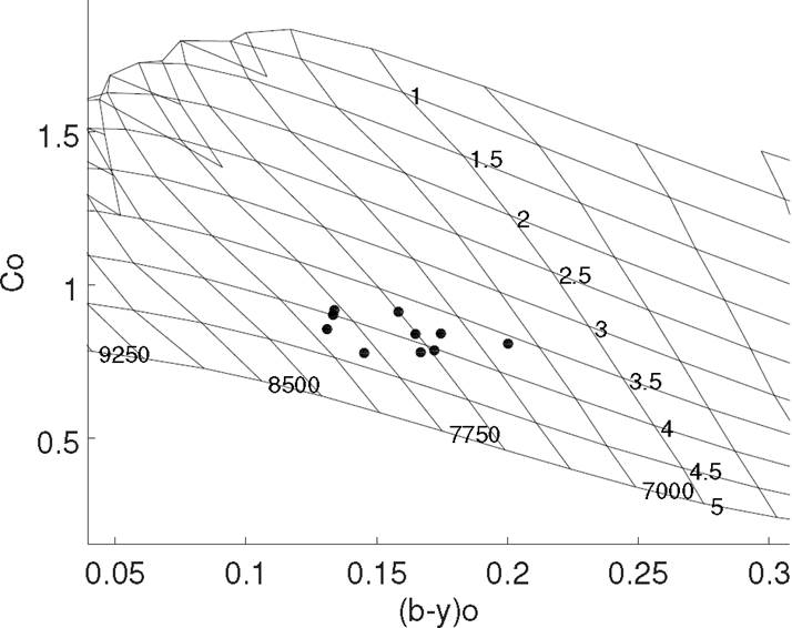
Subsequent columns present metallicity, effective temperature from the theoretical relation reported by Rodriguez (1989) based on a relation from Petersen & Jorgensen (1972, hereinafter P&J72) Te = 6850 + 1250 × (β − 2.684)/0.144 for each value and averaged, and suface gravity. The averaged temperature along the phase interval of 0.3 to 0.8 is 7682 ± 503 K.
4.3. Physical Parameters Conclusions
Most of the papers devoted to BL Cam have emphasised its pulsational nature and few have tried to determine its physical parameters. In this paper, we were able to unredden the color indexes and determine the reddening and the metallicity with uvby − β photoelectric photometry and the well-calibrated equations of Nissen (1988). Locating these indexes on the grids of Castelli & Kurucz (2006) we determined the effective temperature and surface gravity of the star along its cycle of pulsation.
TABLE 11 COLOR INDEXES & PHYSICAL PARAMETERS OF BL CAM AS A FUNCTION OF PHASE
| HJD - 2458900.0 | (b−y) 0 | m 0 | c0 | β | [Fe/H] | Te[K] | logg | Phase |
|---|---|---|---|---|---|---|---|---|
| 6.7315 | 0.067 | 0.090 | 0.979 | 2.865 | 8421 | 3.9 | 0.54 | |
| 4.6828 | 0.093 | 0.123 | 0.739 | 2.863 | 8403 | 4.7 | 0.14 | |
| 6.6732 | 0.104 | 0.156 | 0.798 | 2.842 | 8221 | 4.3 | 0.05 | |
| 4.6872 | 0.102 | 0.105 | 0.858 | 2.838 | 8186 | 4.1 | 0.26 | |
| 6.6754 | 0.110 | 0.199 | 0.807 | 2.835 | 8160 | 4.3 | 0.11 | |
| 4.6956 | 0.103 | 0.164 | 0.892 | 2.834 | 8152 | 4.0 | 0.47 | |
| 6.7452 | 0.110 | 0.112 | 0.802 | 2.834 | 8152 | 4.3 | 0.89 | |
| 6.7516 | 0.114 | 0.112 | 0.769 | 2.834 | 8152 | 4.4 | 0.06 | |
| 4.6898 | 0.100 | 0.123 | 0.946 | 2.830 | 8117 | 3.8 | 0.32 | |
| 6.7331 | 0.107 | 0.097 | 0.895 | 2.827 | 8091 | 3.9 | 0.58 | |
| 4.6674 | 0.107 | 0.038 | 0.898 | 2.824 | 8065 | 3.8 | 0.75 | |
| 4.7295 | 0.116 | 0.139 | 0.848 | 2.824 | 8065 | 4.1 | 0.34 | |
| 6.6908 | 0.119 | 0.145 | 0.855 | 2.819 | 8021 | 4.1 | 0.50 | |
| 6.6937 | 0.109 | 0.157 | 0.970 | 2.817 | 8004 | 3.6 | 0.58 | |
| 6.7501 | 0.125 | 0.100 | 0.802 | 2.817 | 8004 | 4.2 | 0.02 | |
| 4.7039 | 0.127 | 0.157 | 0.850 | 2.809 | 7935 | 4.0 | 0.68 | |
| 4.7354 | 0.119 | 0.053 | 0.963 | 2.805 | 7900 | 3.6 | 0.49 | |
| 4.6982 | 0.130 | 0.094 | 0.857 | 2.804 | 7891 | 3.9 | 0.54 | |
| 4.7130 | 0.135 | 0.033 | 0.799 | 2.804 | 7891 | 4.1 | 0.91 | |
| 4.6857 | 0.144 | 0.087 | 0.792 | 2.794 | 7804 | 4.1 | 0.22 | |
| 4.7069 | 0.143 | 0.060 | 0.849 | 2.788 | 7752 | 3.8 | 0.76 | |
| 4.6785 | 0.156 | 0.087 | 0.750 | 2.785 | 7726 | 4.2 | 0.03 | |
| 4.6690 | 0.157 | 0.075 | 0.747 | 2.784 | 7718 | 4.1 | 0.79 | |
| 4.7202 | 0.155 | 0.124 | 0.791 | 2.782 | 7700 | 4.0 | 0.10 | |
| 6.7438 | 0.155 | 0.141 | 0.788 | 2.782 | 7700 | 4.0 | 0.86 | |
| 4.7145 | 0.165 | 0.131 | 0.696 | 2.781 | 7692 | 4.3 | 0.95 | |
| 4.7408 | 0.156 | 0.130 | 0.814 | 2.778 | 7665 | 3.9 | 0.63 | |
| 6.6922 | 0.151 | 0.111 | 0.870 | 2.778 | 7665 | 3.7 | 0.54 | |
| 6.7208 | 0.147 | 0.128 | 0.918 | 2.777 | 7657 | 3.6 | 0.27 | |
| 4.7024 | 0.153 | 0.084 | 0.871 | 2.774 | 7631 | 3.7 | 0.64 | |
| 6.7467 | 0.164 | 0.115 | 0.789 | 2.771 | 7605 | 3.9 | 0.93 | |
| 4.7423 | 0.164 | 0.111 | 0.832 | 2.766 | 7561 | 3.8 | 0.67 | |
| 4.7085 | 0.165 | 0.105 | 0.847 | 2.763 | 7535 | 3.7 | 0.80 | |
| 4.7439 | 0.166 | 0.057 | 0.862 | 2.759 | 7501 | 3.6 | 0.70 | |
| 4.7384 | 0.182 | 0.144 | 0.815 | 2.746 | 7388 | 3.7 | 0.56 | |
| 4.7241 | 0.200 | 0.118 | 0.821 | 2.719 | -0.775 | 7153 | 3.4 | 0.20 |
| 6.6771 | 0.200 | 0.081 | 0.763 | 2.717 | -1.314 | 7136 | 3.6 | 0.15 |
| 4.7370 | 0.187 | 0.039 | 0.933 | 2.716 | -1.939 | 7127 | 2.9 | 0.53 |
| 4.6939 | 0.194 | 0.091 | 0.963 | 2.713 | -1.121 | 7101 | 2.8 | 0.43 |
| 4.6767 | 0.203 | 0.056 | 0.838 | 2.702 | -1.539 | 7006 | 3.1 | 0.99 |
| 6.7530 | 0.217 | 0.096 | 0.759 | 2.697 | -0.937 | 6962 | 3.4 | 0.09 |
| 4.7478 | 0.217 | 0.060 | 0.880 | 2.681 | -1.334 | 6823 | 2.8 | 0.81 |
| 4.6719 | 0.225 | 0.068 | 0.779 | 2.679 | -1.221 | 6806 | 3.1 | 0.86 |
| 4.6735 | 0.226 | 0.041 | 0.817 | 2.665 | -1.518 | 6685 | 2.8 | 0.90 |
| 4.6814 | 0.257 | 0.077 | 0.804 | 2.643 | -1.068 | 6494 | 2.7 | 0.11 |
| 4.6914 | 0.259 | 0.097 | 0.944 | 2.643 | -0.837 | 6494 | 2.3 | 0.36 |
| 4.7453 | 0.252 | 0.054 | 0.860 | 2.635 | -1.322 | 6424 | 2.5 | 0.74 |
| 4.7493 | 0.268 | 0.062 | 0.786 | 2.623 | -1.244 | 6320 | 2.6 | 0.84 |
| Average | -1.244 | 7598 | ||||||
| σ | 0.315 | 555 |
5. CONCLUSIONS
In the present study we have demonstrated that BL Cam is pulsating with one stable varying period whose O−C residuals show a sinusoidal pattern compatible with a light-travel time effect.
We have shown that the evolution of the ephemerides of the different authors were natural and correct given the shortness of the available data at their times. With a longer time basis we have shown that the long term variation is due to a binary system.
For the determination of the physical parameters some authors mentioned the need to acquire data in uvby − β , a need that we were able to satisfy. New observations in uvby−β and CCD photometry were carried out at the San Pedro Mártir and Tonantzintla observatories, respectively, on the SX Phe star BL Cam.
The appropriate model of Castelli & Kurucz (2006) provided the physical characteristics of the star: effective temperature (T e ) and surface gravity (logg), once the metallicity had been determined. The effective temperature was also calculated through the theoretical relation (P&J72). The numerical values obtained by both methods gave similar results within the error bars, and gave a good idea of the behavior of the star.

