Articles
Stability analysis of relativistic polytropes
Abdel-Naby S. Saad1
2
Mohamed I. Nouh2
Ashraf A. Shaker2
Tarek M. Kamel2
1 Department of Mathematics, Deanship of
Educational Services, Qassim University, Buraidah, Saudi Arabia.
2 Astronomy Department, National Research
Institute of Astronomy and Geophysics(NRIAG), 11421 Helwan, Cairo,
Egypt.
ABSTRACT
We study the relativistic self-gravitating, hydrostatic spheres with a polytropic
equation of state, considering structures with the polytropic indices
n = 1(0.5)3 and illustrate the results for
the relativistic parameters σ = 0 − 0.75. We
determine the critical relativistic parameter at which the mass of the polytrope
has a maximum value and represents the first mode of radial instability. For
n = 1(0.5)2.5, stable
relativistic polytropes occur for σ less than the critical
values
0.42,0.20,0.10,
and 0.04, respectively, while unstable relativistic polytropes
are obtained when σ is greater than the same values. When
n = 3.0 and σ >
0.5, energetically unstable solutions occur. The results of
critical values are in full agreement with those evaluated by several authors.
Comparisons between analytical and numerical solutions of the given relativistic
functions provide a maximum relative error of order 10−3.
Key Words: methods; analytical; methods; numerical; stars; interiors
RESUMEN
Estudiamos esferas hidrostáticas, autogravitantes y relativistas, con una
ecuación de estado politrópica, considerando estructuras con índices
politrópicos n = 1(0.5)3, e ilustramos los
resultados para parámetros relativistas σ = 0 −
0.75. Determinamos el parámetro relativista crítico, para
el cual la masa del politropo alcanza un valor máximo y representa el primer
modo de inestabilidad radial. Con n =
1(0.5)2.5 encontramos politropos
relativistas estables para σ menor que los valores críticos
0.42,0.20,0.10,
y 0.04, respectivamente. Se obtienen politropos relativistas
inestables para valores mayores de σ. Cuando n
= 3.0 y σ > 0.5
encontramos soluciones energéticamente inestables. Los resutados sobre los
valores críticos concuerdan muy bien con los de otros autores. Al comparar las
soluciones analíticas y numéricas de las funciones relativistas estudiadas se
encuentran errores relativos máximos del orden de 10−3.
1. INTRODUCTION
Polytropic models could be considered simple models of stellar structure, and we have
all of the equations needed to make more sophisticated stellar models by solving the
equations of stellar structure. However, there is a need to ask whether the
calculated models provide stable spherically symmetric models.
Several authors have investigated the stability of the polytropic models. Bonnor (1958) found that self-gravitating,
polytropic spheres with n = 3 were inconditionally stable to radial
perturbations. For the first time, Chandrasekhar
(1964) provided the radial stability equation. Earlier methods used to
examine the stability of polytropic stars are listed in Bardeen et al. (1966). More recently, the stability of
polytropes with different polytropic indices was described by Horedt (2013) and Raga et al.
(2020).
In stellar structures such as white dwarfs, neutron stars, black holes and
supermassive stars, and in star clusters, relativistic effects play a significant
role
(Sen and Roy 1954, Sharma 1988). Tooper
(1964) performed a relativistic analysis of the polytropic equation of
state and derived the non-relativistic Lane-Emden equation from two nonlinear
differential equations (Tolman-Oppenheimer, TOV). The problem of the stability of
relativistic stars has long been investigated in the literature, for example, by
Zeldovich and Novikov (1978), Shapiro and
Teukolsky (1984), Takatsuka and Tamagaki
(1993), Casalbuoni and Nardulli
(2004), Khalilov (2002), Isayev (2015), Chu et al. (2015).
In the present paper, we examine the stability of the relativistic polytrope for
different polytropic indices. An analytical solution to the TOV equation is
introduced, which provides the physical parameters of the relativistic polytrope. We
investigate the critical values of the relativistic parameter for which the onset of
the radial instability occurs. The structure of the paper is as follows: § 2 is
devoted to the formulation of the TOV equation. In § 3 we give a brief description
of the analytical method used to solve the TOV equation. § 4 deals with the obtained
results. The conclusion is outlined in § 5.
2. THE EQUATION OF HYDROSTATIC EQUILIBRIUM
The interior of a symmetric star can be described in a spherical coordinate system
(r,ϑ,ϕ) by the standard form of the metric (Tolman 1939, Landu & Lifshitz 1975)
ds2=eνc2dt2-eλdr2-r2dϑ2-r2sin2ϑdφ2,
(1)
where ν and λ are functions of radius
r. As for a fluid star, the components of the energy momentum
tensor corresponding to the above metric are given by
T00=ρc2eν,T11=Peλ,T22=Pr2,T33=Pr2sin2ϑ,
(2)
where ρ, P and c are the mass
density, pressure, and speed of light, respectively. The time-independent
gravitational equations for the line element equation (1) and the energy momentum
tensor are
e-λ1rdνdr+1r2-1r2=8πGc4P,
(3)
e-λ1rdλdr-1r2+1r2=8πGc4ρc2,
(4)
dPdr=-12P+ρc2dνdr,
(5)
where G = 6.67×10⁻⁸
g
−1 cm3 s−2 is the Newtonian gravitational constant.
Equations (3), (4), and (5) together with the equation of state ρ =
ρ(P) represent the hydrostatic equilibrium for
an isotropic general relativistic fluid sphere and can be solved to get
λ, ν, P and
ρ as functions of r. For hydrostatic
equilibrium stars, the Tolman-Oppenheimer-Volkoff (TOV) general relativity equation
obtained by solving Einstein’s field equations has the form
dPdr=-Gε(r)m(r)c2r2[1+P(r)ε(r)][1+4πr3P(r)m(r)c2][1-2Gm(r)c2r]-1,
(6)
where
mr=∫0r4πρrr2dr,
is the gravitational mass interior to radius r and
ε(r) is the internal energy density.
Equation (6) is an extension of the Newtonian formalism with a relativistic
correction. The equation of state for a polytropic star is P =
Kρ
1+
n
1 , where n is the polytropic index. Tooper (1964) has shown that the TOV equation
together with the mass conservation equation have the form
ξ2dθdξ1-2σ(n+1)υ/ξ1+σθ+υ+σξθdυdξ=0,(7)
and
dυdξ=ξ2θn,
(8)
with the initial conditions
θ(0)=1,υ(0)=0,
(9)
Where
θ =ρ / ρ c, ξ =rA, υ =A3 mr4π ρ c ,A=4πGρ cσn+1c21/2, σ=Pcρcc2 =Kρc1/nc2 ,
(10)
σ is the relativistic parameter that can be related to the sound
velocity in the fluid, because the sound velocity is given by υs2=dPdρ in an adiabatic expression. In equations (10) θ, ξ and
υ are dimensionless parameters, while A is a
constant.
If the pressure is much smaller than the energy density at the center of a star (i.e.
σ tends to zero), then equation (7) reduces to
ξ2dθdξ+υ=0.
(11)
Equation (8) together with equation (11) reproduce the well-known Lane-Emden equation
for Newtonian polytropic stars
1ξ2ddξξ2dθdξ+θn=0.
(12)
When n tends to zero, we obtain the case of incompressible matter,
for which the analytic solutions are possible in both relativistic and
nonrelativistic cases. The nonrelativistic Lane-Emden equation has an analytical
solution in closed form only for n = 0, 1 and 5.
However, this is not possible for the relativistic equation, and numerical
integrations must be performed (Tooper 1964;
Bludman 1973; Ferrari et al. 2007).
3. ANALYTICAL SOLUTIONS OF THE RELATIVISTIC EQUATIONS
Nouh (2004)), Nouh and Saad (2013) introduced a new analytical solution of equations
(7-8) applying the Euler-Abel transformation (Demodovich & Maron, 1973) and then a Pade approximation to the
Euler-Abel transformed series (Appendix B) to
accelerate the convergence of the power series solutions.
In this paper, we analyze the gravitational stability of polytropic fluid spheres
based on the analytical solution of the TOV equations that have already been given
by Nouh and Saad (2013). We consider the
cases of polytropic index n =
3.0,2.5,2.0,1.5,
and 1.0 for σ < n/(n + 1).
The analytical solution has the form:
θξ=1+∑k=1∞akξ2k,
(13)
where
ak+1=σ2(k+1)(2(n+1)γk-1-ηk-βk+σζk)-αk2(k+1)(2k+3), k≥1,γk-1=∑i=0k-1figk-i-1, ηk=∑i=0kaigk-i,βk=∑i=0kaiαk-i, ζk=∑i=0kaiβk-i,fi=2(i+1)ai+1, gi=αi(2i+3), γk=∑i=0kfigk-i,αk=1ka0∑i=1k(ni-k+i)aiαk-i, k≥1,α0=a0n,anda0=1.
(14)
From equations (10), for some values of n, σ and
ρ
c
we can determine K, and obtain the radius R
and the mass M(R) from
R=A-1ξ1=c24πGn+1σ1-nKc2n1/2ξ1,
(15)
M=4πρcA3νξ1=14πn+1c2G3Kc2n1/2M~,
(16)
M~≡σ3-n/ 2νξ1 .
(17)
ξ
1 is the first zero of the Lane-Emden function
θ(ξ); equation (8), can be written in the
form
υ(ξ1)=∑k=0∞αk(2k+3)ξ12k+3.
(18)
The power series solution, equation (13), converges rapidly for values of the
polytropic index n ≤ 2 and the error between analytical and
numerical solutions is of order 10−4. For n > 2, the
series solution utilized gives a slow convergence, and the calculation of the
stellar mass from equations (16) and (17) indicates a larger error. The physical
range for a convergent power series can be extended with a change of the independent
variable. Transformations by changing the independent variable are utilized to
improve and accelerate the series convergence in equation (18) for n
> 2 (Pasucal 1977, Saad 2004):
x=6*1+13ξ21\2.
(19)
4. RESULTS
The results evaluated by the use of equations in § 3 are utilized here to analyze the
stability of relativistic polytropes for various values of the general relativity
parameter σ and polytropic index n. The numerical
results obtained are tabulated in Appendix A
for n = 1(0.5) to 3.0 and a range
of values of σ. Comparisons of the analytical solutions of equation
(1) and M̃ (σ) to the numerical method are given
in Tables 5 to 9. Table 10 shows the
critical values of M̃ (σ) due to relativistic
effects for different polytropic indices.
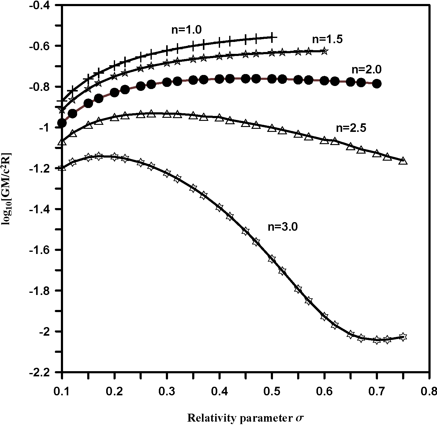
In Figures 1 to 5 we plot M̃ , equation (17), as a function of the
index n and the relativistic effect σ. The figures
show an increase of M̃ (consequently an increase of the stellar
mass M) with σ up to some maximum values (say,
σ
CR
). It is worth mentioning that the critical value σ
CR
marks the onset of the first mode of radial instability. For the case
n = 1.0, Figure
1 shows that the critical value σ
CR
= 0.42, and the relativistic polytropes are stable for
σ < 0.42. In Figures 2, 3, and 4 we observe critical values of the general
relativity index σ
CR
= 0.2, σ
CR
= 0.1 and σ
CR
= 0.04 for the cases n =
1.5, n = 2.0 and
n = 2.5 respectively. In Figure 5 where n = 3.0, M~ has a maximum at σ
CR
= 0 which marks the onset of the first mode of instability, while the minimum
value at σ
CR
= 0.53 marks the onset of the next mode of nonradial
instability. In this case, equation (17) reduces to M̃ ≡
ν(ξ
1). We conclude that for σ
CR
> 0.5 the relativistic polytropic models are
energetically unstable.
The study of the stability of polytropes is useful for determining some physical
properties, such as the maximum mass limit, and illustrates how the stellar mass
increases or decreases due to the effects of general relativity. For a given mass,
radius, and a polytropic index n, Figure 6 of the massradius relation can be used to determine the
internal structure of a polytrope. This means that each value of a relativistic
parameter σ corresponds to a certain internal structure. We can see
from Figure 6 that one pair of mass and radius
corresponds to two different values of σ. For the case of a
polytropic index n = 3.0, the logarithmic function
log10[σ (n +
1)υ(ξ
1)/ξ
1)] = −2.03 has two values of σ ≃
0.67 and σ ≃ 0.75. Then we
have two spherical polytropic configurations of the same mass and radius, but with
different internal structures. When n = 2.0, the
logarithmic function log10[σ (n +
1)υ(ξ
1)/ξ
1)] = −0.76 has two values of σ '
0.42 and σ ' 0.47. Such
information reflects the importance of relativistic solutions.
Table 1 gives the limits of the mass-radius
relations; for example, if the polytropic index n=1.0GM/GMc2R¯c2R¯≤0.214, then the gravitational radius 2GM/c
2 is at most 43% of the invariant(physical) radius R.
When the polytropic index n=3.0 GMc2R¯≤0.072 then the gravitational radius 2GM/c2 is at most
14.5% of the invariant radius R¯ , which is very small compared to the limit value when
n = 1.0.
TABLE 1 LIMITS OF THE MASS-RADIUS RELATIONS
|
n
|
Max. value of log10 σn+1υξ1/ξ1¯
|
Limit ratio of GM/ c2R¯
|
Limit ratio of GM/ c2R
|
| 1.0 |
-0.670
|
0.214 |
0.277 |
| 1.5 |
-0.769
|
0.170 |
0.237 |
| 2.0 |
-0.885
|
0.130 |
0.174 |
| 2.5 |
-1.022
|
0.095 |
0.117 |
| 3.0 |
-1.201
|
0.0633 |
0.072 |
The results of all critical values obtained in this paper for different polytropic
indices are in full agreement with those evaluated by several authors such as Tooper(1964), Bludman(1973), and Araujo & Chirenti
(2011). These critical values σ
CR
and M̃ (σ) together with various indices
n are given in Table 10
(Appendix A). It is shown that the
spherical polytrope of index n = 3.0 and σ
> 0.5 is energetically unstable.
The mass-radius relation (Tooper 1964) has the
form:
GMc2R¯=σ(n+1)υ(ξ1)ξ1¯,
(20)
where R¯ defines the physical radius (invariant radius) of the sphere and ξ1¯=AR¯can be obtained by integrating the equation
ξ1-=∫0ξ1 (1-2σ (n+1)υ(ξ)/ξ-1/2 d ξ.
(21)
The mass-radius relation is useful for determining the surface redshift. It gives the
ratio of the gravitational radius 2GM/c
2 to the invariant radius R¯ when n and σ are known. Rewrite
equation (20) in terms of numerical values for solar mass and solar radius and take
logarithms of both sides of the resulting equation (Tooper, 1964). Then using the solutions introduced in § 3, we plotted
the logarithmic ratio of gravitational radius to a geometrical radius as a function
of the relativistic parameter for different values of the polytropic index
n (see Figure 6). Table 1 gives the limits of the mass-radius
relations for different polytropic index n.
5. SERIES CONVERGENCE
The power series solution of the relativistic problem without using any acceleration
techniques is very limited. Tables 2, 3, and 4
show the radius of convergence ξ
1 of the power series solution (1) of equation (13) and the
relative error (ε) before performing any acceleration. For the
polytropic indices n = 1.0 and n
= 1.5, the series is rapidly convergent. However, beyond these
values, the power series solution is either slowly convergent or divergent. Note
that the relative error (ε = |ξ
1 (An) − ξ
1 (Num)|/ξ
1 (Num)) increases gradually with relativistic effect
σ and polytropic index n. This in turn results
in a small physical range for the convergent power series solutions, and may produce
inaccurate physical parameters of the relativistic polytropes.
TABLE 2 RADII OF CONVERGENCE OF θ(ξ) AND
RELATIVE ERROR FOR n = 1.0
| σ |
ξ
1(N) |
ξ
1(A) |
ε: relative error |
| 0.1 |
2.5990 |
2.5990 |
0.0 |
| 0.2 |
2.2770 |
2.2765 |
0.000219635 |
| 0.3 |
2.0641 |
2.0637 |
0.000193827 |
| 0.4 |
1.9132 |
1.9111 |
0.001098844 |
| 0.5 |
1.8008 |
1.8862 |
0.045276217 |
TABLE 3 RADII OF CONVERGENCE OF θ(ξ) AND
RELATIVE ERROR FOR n = 1.5
| σ |
ξ
1(N) |
ξ
1(A) |
ε: relative error |
| 0.1 |
3.0384 |
3.0730 |
0.011259356 |
| 0.2 |
2.6993 |
2.6025 |
0.037195005 |
| 0.3 |
2.4930 |
2.4281 |
0.026728718 |
| 0.4 |
2.3610 |
2.2648 |
0.042476157 |
| 0.5 |
2.2749 |
2.0644 |
0.101966673 |
| 0.6 |
2.2192 |
1.8340 |
0.210032715 |
TABLE 4 RADII OF CONVERGENCE OF θ(ξ) AND
RELATIVE ERROR FOR n = 2.0
| σ |
ξ
1(N) |
ξ
1(A) |
ε: relative error |
| 0.1 |
3.6989 |
3.4259 |
0.07968709 |
| 0.2 |
3.3983 |
2.5632 |
0.325803683 |
| 0.3 |
3.2711 |
2.5577 |
0.278922469 |
| 0.4 |
3.2473 |
1.9503 |
0.665025893 |
| 0.5 |
3.2967 |
1.9836 |
0.661978221 |
| 0.6 |
3.3986 |
1.7686 |
0.92163293 |
| 0.67 |
3.4982 |
1.6556 |
1.112949988 |
The fourth order Runge-Kutta method was used for the performance of the numerical
solution of the relativistic TOV equation. Analytical and numerical calculations
were done using the Mathematica package, version 11.2.
To extend the physical radii of the convergent power series solutions, a combination
of the two techniques for Euler-Abel transformation and Padé approximation (Nouh 2004; Nouh
& Saad 2013) were utilized. Tables
5 to 9 (Appendix A) show comparisons between numerical and analytical
results. It is worth noting that the power series solutions are rapidly convergent
for polytropic indices n =
1(0.5)3.0 and provide a maximum relative error
of order 10−3.
6. CONCLUSION
In the present paper, we study the stability properties of the relativistic
polytrope. We analyze for various polytropic indices the stability of the
relativistic polytrope. An analytic solution is applied to the TOV equation that
provides us with relativistic polytropic physical parameters. For each polytropic
index, we test the critical values of the relativistic parameter at which the radial
instability started. It is shown that for a given mass, radius and polytropic index
n, the internal structure of a polytropic fluid sphere can be
determined as a function of the relativistic parameter σ. For
n = 1(0.5)2.5, stable
relativistic polytropes occur for σ less than the critical values
0.42,0.20,0.10,
and 0.04, respectively, while unstable relativistic polytropes are
obtained when the relativistic parameter σ is greater than the same
values. When n = 3.0 and σ >
0.5, energetically unstable solutions occur.
We thank the referee for his/her valuable comments which improved the paper.
REFERENCES
Araujo, F. M. & Chirenti, C. B. M. H. 2011,
arXiv:1102.2393
[ Links ]
Bardeen, J. M., Thorne, K. S., & Meltzer, D. W. 1966, ApJ, 145,
505
[ Links ]
Bludman, S. A. 1973, ApJ , 183, 637
[ Links ]
Bonnor, W. B. 1958, MNRAS, 118, 523
[ Links ]
Casalbuoni, R. & Nardulli, G. 2004, RvMP, 76,
263
[ Links ]
Chandrasekhar, S. 1964, ApJ , 140, 417
[ Links ]
Chu, P. Ch., Wang, X., Chen, L. W., & Huang, M. 2015, PhRvD, 91,
3003
[ Links ]
Demidovich, B. P. & Maron, I. A. 1973, Computational
Mathematics, 519.4, D4
[ Links ]
Ferrari, L., Estrela, G., & Malheiro, M. 2007, IJMPE, 16,
2834
[ Links ]
Horedt, G. P. 2004, Polytropes-Applications in Astrophysics and
Related Fields, Astrophysics and Space Science Library 306 (Dordrecht:
Springer)
[ Links ]
Horedt, G. P. 2013, ApJ , 773, 131
[ Links ]
Isayev, A. A. 2015, PhRvC, 91, 5208
[ Links ]
Khalilov, V. R. 2002, PhRvD , 65, 6001
[ Links ]
Landau, L. D. & Lifshitz, E. M. 1975, The classical theory of
fields (2nd ed; Reading, MA: Addison-Wesley Publishing Co.)
[ Links ]
Nouh, M. I. 2004, NewA, 9, 467
[ Links ]
Nouh, M. I. & Saad, A. S. 2013, International Review of Physics,
7(1), 16
[ Links ]
Pascual, P. 1977, A&A, 60, 161
[ Links ]
Raga, A. C., Osorio-Caballero, J. A., Chan, R. S., et al. 2020,
RMxAA, 56, 55
[ Links ]
Saad, A. S. 2004, AN, 325, 733
[ Links ]
Sen, N. R. & Roy, T. C. 1954, ZA, 34, 84
[ Links ]
Shapiro, S. L. & Teukolsky, S. A. 1983, Black-holes, white
dwarfs and neutron stars: the physics of compact objects (New York, NY:
Wiley)
[ Links ]
Sharma, J. P. 1988, ApJ , 329, 232
[ Links ]
Takatsuka, T. & Tamagaki, R. 1993, PthPS, 112,
27
[ Links ]
Tolman, R. C. 1939, PhRv, 55, 364
[ Links ]
Tooper, R. F. 1964, ApJ , 140, 434
[ Links ]
Zeldovich, Y. B. & Novikov, I. D. 1978, Relativistic
Astrophysics, Vol. I: Stars and relativity (Chicago, IL: University of Chicago
Press)
[ Links ]
APPENDIX A: NUMERICAL RESULTS
In the following tables, we list the numerical results obtained for different
polytropic indices. The designation of the columns are as follows:
1. σ: |
is the relativistic parameter. |
2. ξ
1: |
is the first zero of the Emden function. |
3. ν(ξ
1)
Num
: |
is the numerical solution of the relativistic function. |
4. ν(ξ
1)
An
: |
is the analytical solution of the relativistic function. |
5. M̃ (σ)
Num
: |
is a parameter analog to the mass of the polytrope computed
numerically. |
6. M̃ (σ)
An
: |
is a parameter analog to the mass of the polytrope computed
analytically. |
7. ∆ν(ξ
1)
Num
: |
is the difference between the analytical and the numerical values of
the function. |
8. ∆M̃ (σ)
An
: |
is the difference between the analytical and the numerical
values. |
9. σ
critical
: |
is the critical value of the fractional parameter at which
instability started. |
TABLE 5 COMPARISONS BETWEEN ANALYTICAL AND NUMERICAL SOLUTIONS OF THE
RELATIVISTIC FUNCTIONS (1) AND M̃
(σ) FOR n =
1.0
| σ |
ξ1 |
ν(ξ1)Num
|
ν(ξ1)An
|
M̃(σ)Num
|
M̃(σ)An
|
∆ν(ξ1)Num
|
∆M̃(σ)An
|
| 0.0 |
3.1415 |
3.1416 |
3.1416 |
0.0 |
0.0 |
0.0 |
0.0 |
| 0.10 |
2.5990 |
1.7514 |
1.7514 |
0.1751 |
0.1751 |
0.0 |
0.0 |
| 0.12 |
2.5221 |
1.5922 |
1.5922 |
0.1911 |
0.1911 |
0.0 |
0.0 |
| 0.15 |
2.4198 |
1.3941 |
1.3941 |
0.2091 |
0.2091 |
0.0 |
0.0 |
| 0.17 |
2.3590 |
1.2834 |
1.2835 |
0.2182 |
0.2182 |
0.0001 |
0.0 |
| 0.20 |
2.2770 |
1.1426 |
1.1426 |
0.2285 |
0.2285 |
0.0 |
0.0 |
| 0.22 |
2.2278 |
1.0624 |
1.0624 |
0.2337 |
0.2337 |
0.0 |
0.0 |
| 0.25 |
2.1607 |
0.9585 |
0.9585 |
0.2396 |
0.2396 |
0.0 |
0.0 |
| 0.27 |
2.1200 |
0.8983 |
0.8981 |
0.2425 |
0.2425 |
0.0002 |
0.0 |
| 0.30 |
2.0641 |
0.8192 |
0.8190 |
0.2457 |
0.2457 |
0.0002 |
0.0 |
| 0.32 |
2.0299 |
0.7727 |
0.7728 |
0.2473 |
0.2473 |
-0.0001 |
0.0 |
| 0.35 |
1.9827 |
0.7109 |
0.7109 |
0.2488 |
0.2488 |
0.0 |
0.0 |
| 0.37 |
1.9536 |
0.6742 |
0.6742 |
0.2495 |
0.2495 |
0.0 |
0.0 |
| 0.40 |
1.9132 |
0.6249 |
0.6250 |
0.2500 |
0.2500 |
0.0001 |
0.0 |
| 0.42 |
1.8882 |
0.5954 |
0.5954 |
0.2501 |
0.2501 |
0.0 |
0.0 |
| 0.45 |
1.8531 |
0.5553 |
0.5554 |
0.2499 |
0.2499 |
0.0001 |
0.0 |
| 0.47 |
1.8314 |
0.5311 |
0.5310 |
0.2496 |
0.2496 |
0.0001 |
0.0 |
| 0.50 |
1.8008 |
0.4981 |
0.4981 |
0.2491 |
0.2491 |
0.0 |
0.0 |
TABLE 6 COMPARISONS BETWEEN ANALYTICAL AND NUMERICAL SOLUTIONS OF THE
RELATIVISTICFUNCTIONS (1) AND M̃
(σ) FOR n =
1.5
|
σ
|
ξ1
|
νξ1Num
|
νξ1An
|
M~σNum
|
M~σAn
|
ΔM~σAn
|
| 0.0 |
3.6537 |
2.7141 |
2.7141 |
0.0 |
0.0 |
0.0 |
| 0.10 |
3.0384 |
1.4823 |
1.4822 |
0.263592 |
0.263569 |
2.3E-05 |
| 0.12 |
2.9552 |
1.3446 |
1.3446 |
0.274153 |
0.274151 |
2E-06 |
| 0.15 |
2.8464 |
1.1744 |
1.1741 |
0.283069 |
0.282987 |
8.2E-05 |
| 0.17 |
2.783 |
1.08 |
1.08 |
0.285922 |
0.285841 |
8.1E-05 |
| 0.20 |
2.6993 |
0.9602 |
0.9602 |
0.287166 |
0.287166 |
0.0 |
| 0.22 |
2.65 |
0.8925 |
0.8921 |
0.286706 |
0.286558 |
0.000148 |
| 0.25 |
2.5843 |
0.805 |
0.8049 |
0.284609 |
0.284568 |
4.1E-05 |
| 0.27 |
2.5453 |
0.7545 |
0.7543 |
0.282603 |
0.282524 |
7.9E-05 |
| 0.30 |
2.493 |
0.6881 |
0.6881 |
0.278913 |
0.278913 |
0.0 |
| 0.32 |
2.4619 |
0.6496 |
0.6494 |
0.27638 |
0.276292 |
8.8E-05 |
| 0.35 |
2.42 |
0.5982 |
0.5981 |
0.272214 |
0.272151 |
6.3E-05 |
| 0.37 |
2.3949 |
0.5678 |
0.5677 |
0.269366 |
0.269303 |
6.3E-05 |
| 0.40 |
2.361 |
0.5269 |
0.5269 |
0.265018 |
0.265018 |
0.0 |
| 0.42 |
2.3407 |
0.5026 |
0.5025 |
0.262221 |
0.262144 |
7.7E-05 |
| 0.45 |
2.3134 |
0.4696 |
0.4695 |
0.258014 |
0.25794 |
7.4E-05 |
| 0.47 |
2.297 |
0.4497 |
0.4496 |
0.25527 |
0.255216 |
5.4E-05 |
| 0.50 |
2.2749 |
0.4227 |
0.4227 |
0.251326 |
0.251326 |
0.0 |
| 0.52 |
2.2617 |
0.4061 |
0.4061 |
0.248669 |
0.248655 |
1.4E-05 |
| 0.55 |
2.2439 |
0.3835 |
0.3833 |
0.244906 |
0.244817 |
8.9E-05 |
| 0.57 |
2.2333 |
0.3696 |
0.3696 |
0.242484 |
0.242432 |
5.2E-05 |
| 0.60 |
2.2192 |
0.3504 |
0.3504 |
0.238846 |
0.238846 |
0.0 |
TABLE 7 COMPARISONS BETWEEN ANALYTICAL AND NUMERICAL SOLUTIONS OF THE
RELATIVISTIC FUNCTIONS (1) AND M̃
(σ) FOR n =
2.0
|
σ
|
ξ1
|
νξ1Num
|
νξ1An
|
M~σNum
|
M~σAn
|
ΔM~σAn
|
| 0.0 |
4.3531 |
2.411 |
2.411 |
0.0 |
0.0 |
0.0 |
| 0.05 |
3.9617 |
1.7165 |
1.7162 |
0.3838 |
0.3838 |
0.0 |
| 0.07 |
3.8443 |
1.5258 |
1.5258 |
0.4037 |
0.4037 |
0.0 |
| 0.10 |
3.6989 |
1.2987 |
1.2983 |
0.4107 |
0.4106 |
0.0001 |
| 0.12 |
3.6191 |
1.1769 |
1.1766 |
0.4077 |
0.4076 |
0.0001 |
| 0.15 |
3.5198 |
1.0272 |
1.0274 |
0.3978 |
0.3979 |
-0.0001 |
| 0.17 |
3.4653 |
0.9445 |
0.9440 |
0.3894 |
0.3892 |
0.0002 |
| 0.20 |
3.3983 |
0.8403 |
0.8399 |
0.3758 |
0.3756 |
0.0002 |
| 0.22 |
3.3619 |
0.7814 |
0.7815 |
0.3665 |
0.3665 |
0.0 |
| 0.25 |
3.3186 |
0.7058 |
0.7056 |
0.3529 |
0.3528 |
0.0001 |
| 0.27 |
3.2962 |
0.6623 |
0.6622 |
0.3441 |
0.3441 |
0.0 |
| 0.30 |
3.2711 |
0.6055 |
0.6057 |
0.3316 |
0.3318 |
-0.0002 |
| 0.32 |
3.2595 |
0.5723 |
0.5725 |
0.3238 |
0.3239 |
-0.0001 |
| 0.35 |
3.2491 |
0.5285 |
0.5285 |
0.3127 |
0.3127 |
0.0 |
| 0.37 |
3.2463 |
0.5026 |
0.5024 |
0.3057 |
0.3056 |
0.0001 |
| 0.40 |
3.2473 |
0.4680 |
0.4678 |
0.2960 |
0.2959 |
0.0001 |
| 0.42 |
3.2526 |
0.4474 |
0.4478 |
0.2899 |
0.2902 |
-0.0003 |
| 0.45 |
3.2644 |
0.4195 |
0.4196 |
0.2814 |
0.2815 |
-0.0001 |
| 0.47 |
3.2754 |
0.4028 |
0.4030 |
0.2761 |
0.2763 |
-0.0002 |
| 0.50 |
3.2967 |
0.3800 |
0.3804 |
0.2687 |
0.2690 |
-0.0003 |
| 0.52 |
3.3128 |
0.3662 |
0.3668 |
0.2641 |
0.2645 |
-0.0004 |
| 0.55 |
3.3416 |
0.3474 |
0.3468 |
0.2576 |
0.2572 |
0.0004 |
| 0.57 |
3.3632 |
0.3359 |
0.3360 |
0.2536 |
0.2537 |
-0.0001 |
| 0.60 |
3.3986 |
0.3201 |
0.3202 |
0.2479 |
0.2481 |
-0.0002 |
| 0.62 |
3.4253 |
0.3104 |
0.3103 |
0.2444 |
0.2443 |
0.0001 |
| 0.65 |
3.4678 |
0.2970 |
0.2973 |
0.2394 |
0.2397 |
-0.0003 |
| 0.67 |
3.4982 |
0.2887 |
0.2891 |
0.2363 |
0.2366 |
-0.0003 |
TABLE 8 COMPARISONS BETWEEN ANALYTICAL AND NUMERICAL SOLUTIONS OF THE
RELATIVISTIC FUNCTIONS (1) AND M̃
(σ) FOR n =
2.5
|
σ
|
ξ1
|
νξ1Num
|
νξ1An
|
M~σNum
|
M~σAn
|
ΔM~σAn
|
| 0.0 |
5.3552 |
2.1872 |
2.1872 |
0.0 |
0.0 |
0.0 |
| 0.01 |
5.2623 |
2.0281 |
2.0281 |
0.641341 |
0.641341 |
0.0 |
| 0.02 |
5.1793 |
1.88702 |
1.88702 |
0.709633 |
0.709632 |
0.0 |
| 0.03 |
5.1052 |
1.76134 |
1.76131 |
0.733034 |
0.7033021 |
1.3E-05 |
| 0.04 |
5.0393 |
1.648899 |
1.648930 |
0.737410 |
0.737424 |
-1.4E-05 |
| 0.05 |
4.9809 |
1.5479 |
1.548019 |
0.7320 |
0.732013 |
0.0 |
| 0.07 |
4.8841 |
1.3744 |
1.374359 |
0.7069 |
0.706927 |
0.0 |
| 0.10 |
4.7819 |
1.1692 |
1.169269 |
0.6575 |
0.657528 |
0.0 |
| 0.12 |
4.7383 |
1.0599 |
1.059908 |
0.6238 |
0.623826 |
0.0 |
| 0.15 |
4.7044 |
0.9261 |
0.925878 |
0.5764 |
0.576204 |
0.0002 |
| 0.17 |
4.7006 |
0.8527 |
0.852617 |
0.5475 |
0.547477 |
0.0 |
| 0.20 |
4.7206 |
0.7606 |
0.760086 |
0.5086 |
0.508299 |
0.0003 |
| 0.22 |
4.7498 |
0.7088 |
0.708902 |
0.4855 |
0.485503 |
0.0 |
| 0.25 |
4.8163 |
0.6426 |
0.642273 |
0.4544 |
0.454155 |
0.0002 |
| 0.27 |
4.8753 |
0.6048 |
0.605615 |
0.4359 |
0.436554 |
-0.0007 |
| 0.30 |
4.9855 |
0.5556 |
0.554771 |
0.4112 |
0.410576 |
0.0006 |
| 0.32 |
5.0734 |
0.5271 |
0.527703 |
0.3964 |
0.396896 |
0.0005 |
| 0.35 |
5.2273 |
0.4896 |
0.490730 |
0.3766 |
0.377450 |
-0.0009 |
| 0.37 |
5.3450 |
0.4677 |
0.466891 |
0.3648 |
0.364138 |
0.0007 |
| 0.40 |
5.5448 |
0.438571 |
0.444662 |
0.348782 |
0.348982 |
-0.0002 |
| 0.42 |
5.6943 |
0.4214 |
0.421721 |
0.3392 |
0.339499 |
-0.0003 |
| 0.45 |
5.9440 |
0.3984 |
0.397734 |
0.3263 |
0.325758 |
0.0005 |
| 0.47 |
6.1284 |
0.3847 |
0.384457 |
0.3186 |
0.318326 |
0.0003 |
| 0.50 |
6.4335 |
0.3664 |
0.366915 |
0.3081 |
0.308537 |
-0.0004 |
| 0.52 |
6.6569 |
0.3555 |
0.355406 |
0.3019 |
0.301804 |
0.0001 |
| 0.55 |
7.0239 |
0.3408 |
0.340363 |
0.2935 |
0.293112 |
0.0004 |
| 0.57 |
7.2910 |
0.3320 |
0.331352 |
0.2885 |
0.287911 |
0.0006 |
| 0.60 |
7.7273 |
0.3202 |
0.319843 |
0.2818 |
0.281497 |
0.0003 |
| 0.62 |
8.0423 |
0.3131 |
0.319070 |
0.277851 |
0.277888 |
-3.7E-05 |
| 0.65 |
8.5563 |
0.3036 |
0.305345 |
0.2726 |
0.274169 |
-0.0016 |
| 0.67 |
8.9257 |
0.2980 |
0.297274 |
0.2696 |
0.268953 |
-0.0006 |
| 0.70 |
9.5224 |
0.2905 |
0.291442 |
0.2657 |
0.266579 |
-0.0009 |
| 0.72 |
9.9494 |
0.2860 |
0.284817 |
0.2634 |
0.2623610 |
0.001 |
TABLE 9 COMPARISONS BETWEEN ANALYTICAL AND NUMERICAL SOLUTIONS OF THE
RELATIVISTIC FUNCTIONS (1) AND M̃
(σ) FOR n =
3.0.
|
σ
|
ξ1
|
νξ1Num
|
νξ1An
|
M~σNum
|
M~σAn
|
ΔM~σAn
|
| 0.0 |
6.8968 |
2.01824 |
2.01824 |
2.01824 |
2.01824 |
0.0 |
| 0.05 |
6.7074 |
1.42463 |
1.42463 |
1.42463 |
1.42463 |
0.0 |
| 0.07 |
6.7206 |
1.26543 |
1.26542 |
1.26543 |
1.26542 |
1.0E-05 |
| 0.10 |
6.8258 |
1.07845 |
1.07837 |
1.07845 |
1.07837 |
8.0E-05 |
| 0.12 |
6.9521 |
0.979601 |
0.979949 |
0.979601 |
0.979949 |
- 0.0003 |
| 0.15 |
7.2285 |
0.85958 |
0.859491 |
0.85958 |
0.859491 |
9.0E-05 |
| 0.17 |
7.4751 |
0.794229 |
0.793908 |
0.794229 |
0.793908 |
0.0003 |
| 0.20 |
7.9508 |
0.713042 |
0.713880 |
0.713042 |
0.713880 |
-0.0008 |
| 0.22 |
8.3481 |
0.667954 |
0.667963 |
0.667954 |
0.667963 |
-1.0E-05 |
| 0.25 |
9.0894 |
0.611096 |
0.612004 |
0.611096 |
0.612004 |
-0.0009 |
| 0.27 |
9.6994 |
0.579159 |
0.578934 |
0.579159 |
0.578934 |
0.0002 |
| 0.30 |
10.8327 |
0.538631 |
0.540522 |
0.538631 |
0.540522 |
-0.0018 |
| 0.32 |
11.7690 |
0.515833 |
0.519000 |
0.515833 |
0.519000 |
-0.003 |
| 0.35 |
13.5271 |
0.487068 |
0.488563 |
0.487068 |
0.488563 |
-0.001 |
| 0.37 |
15.0007 |
0.471124 |
0.470841 |
0.471124 |
0.470841 |
0.0003 |
| 0.40 |
17.8197 |
0.451585 |
0.452268 |
0.451585 |
0.452268 |
-0.0007 |
| 0.42 |
20.2306 |
0.441299 |
0.443341 |
0.441299 |
0.443341 |
-0.002 |
| 0.45 |
24.9438 |
0.429831 |
0.429350 |
0.429831 |
0.429350 |
0.0005 |
| 0.47 |
29.0538 |
0.424822 |
0.422867 |
0.424822 |
0.422867 |
0.0020 |
| 0.50 |
37.2058 |
0.421395 |
0.421807 |
0.421395 |
0.421807 |
-0.0004 |
| 0.53 |
48.5317 |
0.423168 |
0.418075 |
0.423168 |
0.418075 |
0.0051 |
| 0.60 |
91.0723 |
0.449319 |
0.453089 |
0.449319 |
0.453089 |
-0.004 |
| 0.70 |
162.5832 |
0.526621 |
0.529641 |
0.526621 |
0.529641 |
-0.003 |
| 0.74 |
177.9357 |
0.558153 |
0.554724 |
0.558153 |
0.554724 |
0.003 |
| 0.75 |
180.4379 |
0.565394 |
0.541169 |
0.565394 |
0.541169 |
0.0242 |
TABLE 10 THE CRITICAL VALUES σCR CORRESPONDING
M̃ (σ) FOR VARIOUS INDICES
N
| n |
ξ1
|
σcritical
|
M~σ
|
| 1.0 |
1.8882 |
0.42 |
0.249930 |
| 1.5 |
2.6993 |
0.20 |
0.287166 |
| 2.0 |
3.6989 |
0.10 |
0.410546 |
| 2.5 |
5.0393 |
0.04 |
0.737424 |
| 3.0 |
6.8968 |
0.0 |
2.01824 |
| 3.0 |
48.5317 |
0.53 |
0.416203 |
APPENDIX B. THE SERIES ACCELERATION TECHNIQUE
To accelerate the convergence of the series solution of equation 13, we followed
the scheme developed by Nouh (2004). As
the first step of this scheme, the alternating series is accelerated by
Euler-Abel transformation (Demodovich & Maron
1973).
Let us write
θ(ξ)=a0+ξϕ(ξ),
(22)
where
ϕ(ξ)=∑k=0∞akξk-1=∑k=1∞ak+1ξk;
(23)
then
1-ξϕξ=∑k=0∞ak+1ξk-∑k=1∞akξk=a0+∑k=0∞Δakξk,
(24)
where ∆a
k
= a
k+1
− a
k
,k =
0,1,2,... are finite
differences of the first order of the coefficients a
k
. Applying the Euler-Abel transformation to the power series ∑k=0∞Δakξk, p times, and after some manipulations we
obtain
∑k=0∞akξk=∑i=0∞Δia0ξi1-ξi+1+ξ1-ξp∑k=0∞Δpakξk,
(25)
where ∆0
a
0 = a
0. Equation (25) becomes meaningless when ξ = 1, so,
by setting ξ = −t, we obtain the Euler-Abel
transformed series as
θEnt=∑k=0∞Δia0ti1-ti+1+t1-tp∑k=0∞Δp-1kaktk.
(26)
Returning to the earlier variable, ξ, we obtain
θEn(ξ)=∑i=0p-1(-1)iΔia0ξi(1+ξ)i+ (ξ1+ξ)p∑k=0∞(-1)k+p[Δpak]ξk,
(27)
where
Δpak=Δp-1ak+1-Δp-1ak.
Any order difference ∆
p
a
k
can be written as a linear combination
Δpak=∑i=0p(-1)p-i(pi)ak+1,
where
(pi)=p!i!(p-i)!.
The second step is to apply Padé approximation to the Euler-Abel transformed
series, equation 27.


 nova página do texto(beta)
 Inglês (pdf)
 Artigo em XML
 Referências do artigo
 Enviar este artigo por email
 Citado por SciELO
  Similares em
SciELO
Similares em
SciELO 
 Permalink