


 nueva página del texto (beta)
 Inglés (pdf)
 Artículo en XML
 Referencias del artículo
 Enviar artículo por email
 Citado por SciELO
  Similares en
SciELO
Similares en
SciELO 
 Permalink
1. Introduction
The number of cool spots observed on the solar photosphere fluctuates for the decades of a cycle period. Schwabe (1844) stated the average cycle length as about 11 years. The patterns based on the magnetic field are observed in the case of the late-type stars as well as the solar case (Kron 1950). In the case of the solar analogues, some long-term variations have been discovered from the long-term observations of the Ca II H (λ3968 Å) and K (λ3933 Å) emission lines, as it is in the solar case (Wilson 1978). Considering the solar-stellar relations found by comprehensive studies, the examination of long-term activity cycles leads us to understand how their dynamos work (Baliunas et al. 1995; Rempel 2008).
Flare activity was detected in the sun by Carrington (1859) and Hodgson (1859) for the first time. Flare activity on WX UMa was reported in 1940 (van Maanen 1940), which may be the earliest known stellar flare. The stars exhibiting flare activity are now called UV Ceti type stars (or flare stars). UV Ceti type stars are young stars that have just come to the main sequence. Numerous red dwarf stars in both open clusters and association exhibit flare activity (Mirzoian 1990; Pigatto 1990). A decrease in the number of the flare stars is observed with the increase in the age of the cluster, as an expected result of the Skumanich Law (Skumanich 1972; Marcy & Chen 1992; Pettersen 1991; Stauffer 1991).
Activity level rises with increasing rotational speed, which causes mass loss to
increase. The studies indicate that the solar mass loss is about
To understand the whole flare process in detail, one should compare the flares detected from different types of stars. In this respect, there are several studies in the literature. Some of them have been concentrated on the flare frequencies. For example, Ishida et al. (1991) have described two different flare frequencies as the flare frequencies N 1, which is the flare number per hour, and N 2, which is flare energy emitted to space per second. Leto et al. (1997) have demonstrated that the flare frequency of EV Lac varies from one observing season to the next. However, some other studies have concentrated on the flare energy level or limits. In the early 1970s, Gershberg (1972) described the flare energy spectrum, which depends on the distribution of flare cumulative frequency. The distribution of flare cumulative frequency is almost the most studied examination technique in the literature, even today. Indeed, one can see it in several studies such as Ramsay & Doyle (2015); Davenport (2016); Maehara (2017); Davenport et al. (2019); Tu et al. (2020). Another study has recently been conducted by Dal & Evren (2010, 2011), developing a model based on fitting the distributions of flare equivalent duration versus flare total times in the logarithmic scale, which is called the One Phase Exponential Association (hereafter OPEA) model.
In this study, the results found for the flare and spot activities of V1130 Cyg (KIC
4660977) and V461 Lyr (KIC 6205460) will be presented, which depend on the findings
of their OPEA Models with model parameters and stellar spot migrations. V1130 Cyg
was classified as a variable star by Miller
(1966) for the first time. The V -band brightness has
been given as 12
m
.560, while infrared JHK have been given as 11
m
.124, 10
m
.764, 10
m
.657, respectively (Zacharias et
al. 2005). In the literature, the spectral types of its components have
been given as F7 + K0 IV with orbital period (P) of 0.5625613 day
(Svechnikov & Kuznetsova 1990). The
temperatures of the components have been computed as T
1 = 5587 K and T
2 = 6621 K (Armstrong et al. 2014).
According to Mathur et al. (2017), the
temperature of target is T
eff
= 5674K with log g = 3.942
cm/s2. They estimated the radius and mass of the target as
2. Data and Analyses
The Kepler Mission was devoted to find exo-planets. Indeed, more than 150000 targets were observed (Borucki et al. 2010; Koch et al. 2010; Caldwell et al. 2010). These observations are the most sensitive observations ever made (Jenkins et al. 2010a,b). In the mission, many variables such as eclipsing binaries, chromospheric active or pulsating stars, have been discovered apart from numerous exo-planets (Slawson et al. 2011; Matijevič et al. 2012). There are several spotted and flaring targets among newly discovered eclipsing binaries (Balona 2015). The targets’ data analysed in this study have been taken from the Kepler Database (Slawson et al. 2011; Matijevič et al. 2012). From the database, all available detrended short cadence (hereafter SC) and de-trended long cadence (hereafter LC) data have been taken. The light curves of the targets are shown in Figure 1 for both SC and LC data in different colors.
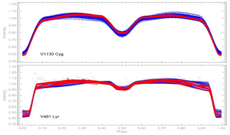
Fig. 1 The light curves of the system are presented. The light curve of V1130 Cyg is shown in the upper panel, that of V461 Lyr in the bottom panel. In both panels, the LC data light curve is plotted as filled blue circles, the SC data light curve as filled red circles. The color figure can be viewed online.
Several spectra have been taken for both targets at the same time, and their data have been provided in the Sloan Digital Sky Surveys (SDSS) archive (Majewski et al. 2017). Both targets have been observed in Apache Point Observatory (APO), using the Sloan 2.5 m Telescope (Gunn et al. 2006). Six spectra have been taken for V1130 Cyg, and four spectra for V461 Lyr. Their data have been released in the database of SDSS IV APOGEE 2 Data Release 16 (DR16) (Ahumada et al. 2019). Although available spectral data do not cover all phases of the targets sufficiently to calculate the radial velocity curve amplitude, considering their orbital periods, the available data suffice to indicate that both targets should be binary stars as it is seen from Figure 2. Using a Python script, depending on the method in the Spectroscopic Binary Solver software (Johnson 2004), we have tried to estimate possible radial velocity curves for the targets over the available data to just make an impression, depending on the fixed orbital periods. In the figure, the observations have been shown by filled circles with their error bars, while the estimated radial velocities are presented by red-dotted lines. According to these estimates, the semi-amplitude (K1) of radial velocity has been found to be about 39.19 km/s−1 for V1130 Cyg, and about 117.79 km/s−1 for V461 Lyr. According to these results, the radial velocity curves of both targets should have been obtained over just one component.

Fig. 2 The radial velocity curves obtained by the Sloan 2.5 m Telescope for both targets. In panels, observations are represented by filled circles with their error bars, while the estimated curves are shown with red-dotted lines. The color figure can be viewed online.
In the study, we have used the Pre-search Data Conditioning Simple Aperture Photometry (PDCSAP) data (Smith et al. 2012; Stumpe et al. 2012) in both SC and LC format for the period (O − C) analyses. For the light curve analyses, we have used LC data for both systems. In the analyses of stellar spot activity, we have used both SC and LC data in a suitable format for V1130 Cyg, while we have used LC data for V461 Lyr. The estimations over the available spectra of the targets have been considered for the light curve analyses, and also for the discussion of the nature of the systems in the last section.
2.1. Orbital Period Variation
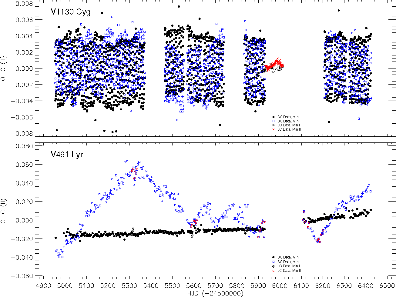
The minima times have been computed from the public SC and LC data taken from the Kepler Database (Slawson et al. 2011; Matijevič et al. 2012) without applying any correction to the observations. In the case of V1130 Cyg, 3249 minima times have been computed from the LC data, while 220 minima times have been obtained from the SC data. In the case of V461 Lyr, 716 minima times have been computed from LC data, and 75 minima from the SC data. We have computed the (O − C) I differences, between the observed minima times and the computed ones. We have obtained the (O − C) I differences for all minima times for both systems. From the data sets of (O − C) I differences, we have extracted all the minima with large error, due to the flare frequencies. We recognized that the purified (O − C) I differences exhibited a linear trend. To remove these trends, we applied a linear corrections to all minima time residuals using equation (1) for V1130 Cyg and equation (2) for V461 Lyr:
After these linear corrections, we have obtained (O − C) II residuals, taking the differences between linear fits and the (O−C) I values. All obtained minima times, their (O −C) I differences and (O − C) II residuals are tabulated in Table 1. When the (O − C) II residuals are plotted versus time, it is seen that the residuals exhibit some systematic variation with time, as shown in Figure 3. In the case of V1130 Cyg, the stellar spot activity occurring on the active component leads the (O − C) II residuals of both the primary and secondary minima to vary synchronously, but in opposite directions, due to the effects presented by Tran et al. (2013) and Balaji et al. (2015). However, it can be seen from the bottom panel of Figure 3 that the secondary minima times are much more affected by spot activity due to their shallower amplitude.
TABLE 1 All the minima times and their r/esiduals for V1130 Cyg and V461 Lyr
| V1130 Cyg | ||||
|---|---|---|---|---|
| HJD | Type | (O − CI) | (O − CII) | |
| (+24 00000) | (day) | (day) | ||
| 54953.77285 | -0.50 | II | 0.0025 | 0.00263 |
| 54954.05240 | 0.00 | I | 0.0007 | 0.00089 |
| 54954.33091 | 0.50 | II | -0.0020 | -0.00187 |
| 54954.61010 | 1.00 | I | -0.0041 | -0.00397 |
| 54954.89837 | 1.50 | II | 0.0029 | 0.00303 |
| 54955.17831 | 2.00 | I | 0.0015 | 0.00169 |
| 54955.45665 | 2.50 | II | -0.0014 | -0.00126 |
| 54955.73540 | 3.00 | I | -0.0039 | -0.00378 |
| 54956.02374 | 3.50 | II | 0.0031 | 0.00328 |
| 54956.30492 | 4.00 | I | 0.0030 | 0.00317 |
| V461 Lyr | ||||
| 54956.46324 | 0.00 | I | 0.0080 | -0.01903 |
| 54958.31067 | 0.50 | II | -0.0060 | -0.03299 |
| 54962.03404 | 1.50 | II | -0.0054 | -0.03241 |
| 54965.75160 | 2.50 | II | -0.0107 | -0.03764 |
| 54969.47630 | 3.50 | II | -0.0088 | -0.03573 |
| 54973.19484 | 4.50 | II | -0.0131 | -0.03998 |
| 54976.91960 | 5.50 | II | -0.0112 | -0.03802 |
| 54980.64768 | 6.50 | II | -0.0060 | -0.03272 |
| 54984.36835 | 7.50 | II | -0.0081 | -0.03484 |
| 54988.08618 | 8.50 | II | -0.0131 | -0.03981 |
2.2. Light Curve Analyses
To detect the absolute light variation of each flare, all the variations such as geometrical effects and sinusoidal variation at out-of-eclipses need to be modelled. To this end, we firstly conducted light curve analyses for both systems. As a first step, we removed the flares from the total light variations, as well as the scattering observations caused by technical problems. Then, for both systems, we chose several consecutive cycles, that were least affected by the spot activity. Lastly, we computed averaged light curves to obtain the data set for the analyses, using the data of these cycles.
We have used the PHOEBE V.0.32 software (Prša & Zwitter 2005), which depends on the Wilson-Devinney Code (Wilson & Devinney 1971; Wilson 1990), to analyse the light curve. We have tried to model the light curve separately by using three modes, such as Mode 2 (detached system), Mode 4 (semi-detached system with the primary component filling its Roche-Lobe), and Mode 5 (semi-detached system with the secondary component filling its Roche-Lobe). Astrophysically acceptable solutions have been found in the analyses with Mode 2 for both systems.
In the light curve analyses, the sinusoidal variations seen at out-of-eclipses have been modelled by two cool spots for the chosen data set. In the analyses, although the third body parameter has been taken as a free parameter, it has been seen that there is no excess of total light due to any third body. The parameters resulting from the light curve analyses are listed in Table 2, while the solutions are shown with the averaged observing data in Figure 4.
TABLE 2 Solution parameters for V1130 Cyg and V461 Lyr*
| Parameter | V1130 Cyg | V461 Lyr |
|---|---|---|
|
|
0.685 |
0.999 |
|
|
90.00 |
89.58 |
|
|
6530 (fixed) | 5774 (fixed) |
|
|
3891 |
4206 |
|
|
0.357 |
0.970 |
|
|
0.376 |
0.428 |
|
|
0.811 |
0.455 |
|
|
0.188 |
0.546 |
|
|
0.32, 0.32 (fixed) | 0.32, 0.32 (fixed) |
|
|
0.50, 0.50 (fixed) | 0.50, 0.50 (fixed) |
|
|
0.64, 0.70 (fixed) | 0.64, 0.664 (fixed) |
|
|
0.616, 0.616 (fixed) | 0.758, 0.751 (fixed) |
|
|
0.3628 |
0.1551 |
|
|
0.2708 |
0.3171 |
|
|
1.135 |
1.135 |
|
|
2.880 |
3.526 |
|
|
0.611 |
0.698 |
|
|
0.900 |
0.900 |
|
|
1.135 |
1.135 |
|
|
0.524 |
6.248 |
|
|
0.436 |
0.436 |
|
|
1.100 |
0.970 |
*Found from the light curve analyses.

Fig. 4 The observed light curves and the synthetic light curve solutions are plotted versus orbital period phases for both V1130 Cyg (upper panel) and V461 Lyr (bottom panel). In the panels, the filled blue circles represent the observations for both systems, while the red lines represent the synthetic curves. The color figure can be viewed online.
2.3. Rotational Modulation and Stellar Spot Activity
In the systems’ light curves, careful examination of the light variations at out-of-eclipses indicates some wave-like sinusoidal variations. Considering both the surface temperature of the components and available flare activities, these wave-like sinusoidal variations must be a stellar rotational modulation caused by the stellar cool spots. It is seen that the minima times of the sinusoidal variations vary when these variations are examined cycle by cycle. This indicates that the active regions exhibit rapid migration on the components’ surfaces. Since it is not possible to model the whole light curves in one step, the data were separated into subsets, considering the shape structures as minima phases, minima, and maxima levels of the consecutive light curves.
In the case of V1130 Cyg, the residuals of the long cadence data have been separated into 30 subsets as described above, which are modelled one by one. In the case of V461 Lyr, the residuals of long cadence data have been modelled in two groups; the deep and shallow minima. In these analyses, the sinusoidal variations have been modelled by using the least squares method to determine their minima times. Then, using these minima times, we have found the migrations of wave-like variation toward the earlier phases in the light curves for both systems.
In the case of V1130 Cyg, examination of the migrations indicates that the active component has one spotted area migrating longitudinally on the stellar surface with a period of 0.33388 years (121.951 d). In the case of V641 Lyr, the analyses have demonstrated that both components have two spotted areas on their surfaces. Two spotted areas on one component migrate with periods of 11.577 and 10.585 years. On the other component, two other spotted areas migrate with periods of 11.807 and 12.836 years. The migrations of all these spots are shown in Figures 5 and 6.
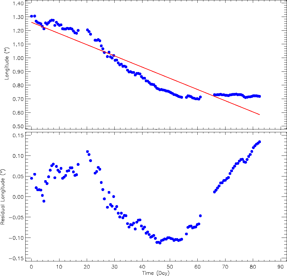
Fig. 5 In the upper panel, the longitudinal variation (filled blue circles) of the stellar cool spot and its linear model for the stellar spots of V1130 Cyg are demonstrated. In the bottom panel, the residuals taken from the linear model are shown. The color figure can be viewed online.

Fig. 6 In the upper left panel, the longitudinal variation of spotted areas on the chromospheric active component of V461 Lyr is shown, while the variation of residuals obtained from the models is exhibited in the lower left panel. In the figure, filled red circles represent the first spot, and filled blue circles the second one. In the upper right panel, the longitudinal variation of the spotted areas on the other component is shown versus time. In the lower right panel, the residuals obtained from the models are shown. The filled blue circles represent the first and the red circles the second spot. The color figure can be viewed online.
2.4. Stellar Flare Activity
To understand the nature of the flare activity and its behaviour on the components, all the variations except the flares in the light curves have been removed. Furthermore, the scattering points due to technical reasons have also been removed from the data.
To determine parameters such as the flare start-end points and the flare equivalent durations, it is necessary to determine the quiescent level of the systems. The sinusoidal light-variations at out-of-eclipses have been modelled by Fourier series. Using these synthetic models, the quiescent level for each flare has been defined. Using the available data in the Kepler Database, 94 flares from V1130 Cyg and 254 flares from V461 Lyr have been detected. The parameters have been calculated for each flare. Two flare examples and their quiescent levels identified by Fourier analysis are shown in Figure 7.

Fig. 7 The flare examples detected from V1130 Cyg (top panel) and V461 Lyr (bottom panel) are shown. In the panels, the filled circles show the observations, while the red lines show the quiescent level defined by Fourier analysis for each light curve part of the targets. The color figure can be viewed online.
After determining the flare start and end times, the flare parameters such as flare maximum time, equivalent duration (P), flare rise (T r ) and decay (T d ) times, flare total time (T t ) and flare amplitude were calculated for each flare. All these parameters are tabulated in Table 3. The time error has been about ±10−8 day for the observation times given in the Kepler Database (Jenkins et al. 2010a,b). Therefore, the error values of the flare time scales have been about ±0.0001 day (±8.64 s). The error values of the computed flare equivalent durations are given in the table for each listed flare. In general, the minimum error value has been found to be ±0.001 s for both targets. The maximum error values have been found to be ±1.006 s for V461 Lyr and ±1.030 s for V1130 Cyg. At this point, it should be noted that equivalent durations of all flares have been calculated by equation (3) defined by Gershberg (1972):
where P is the flare equivalent duration in seconds, the I flare is the flux at the flare moment, and I 0 is the quiescent level flux of the system calculated by the Fourier series at out-of-eclipses. Considering the reasons explained by Dal & Evren (2010, 2011), the flare energies have not been calculated. The equivalent duration parameter has been used instead of the flare energy parameter in the subsequent models.
TABLE 3 PARAMETERS CALCULATED FOR EACH FLARE FOR V1130 CYG AND V461 LYR*
| Flare Time | Amplitude | ||||
|---|---|---|---|---|---|
| (+2400000) | ( |
( |
( |
( |
(Intensity) |
| V1130 Cyg | |||||
| 55933.033204 | 2.871 |
647.313120 | 706.166208 | 1353.479328 | 0.004747 |
| 55933.093141 | 0.772 |
647.304480 | 58.853952 | 706.158432 | 0.001733 |
| 55933.305644 | 0.928 |
353.096928 | 1000.391904 | 1353.488832 | 0.001241 |
| 55933.402359 | 0.375 |
294.224832 | 294.242976 | 588.467808 | 0.001498 |
| 55933.843711 | 5.487 |
470.769408 | 2177.338751 | 2648.108160 | 0.002957 |
| 55933.877766 | 0.878 |
588.476448 | 706.159296 | 1294.635744 | 0.002133 |
| 55934.114788 | 0.621 |
882.702144 | 176.535072 | 1059.237216 | 0.001674 |
| 55934.154291 | 0.381 |
294.242976 | 470.769408 | 765.012384 | 0.001469 |
| 55935.054703 | 2.688 |
176.543712 | 1824.259968 | 2000.803680 | 0.005598 |
| 55935.314883 | 0.051 |
58.853952 | 58.836672 | 117.690624 | 0.000856 |
| V461 Lyr | |||||
| 54962.714192 | 26.897 |
5296.624128 | 15889.872384 | 21186.496512 | 0.002636 |
| 54962.918537 | 2.003 |
1765.540800 | 3531.083328 | 5296.624128 | 0.000497 |
| 54973.871418 | 29.043 |
3531.065184 | 14124.295296 | 17655.360479 | 0.004381 |
| 54974.096197 | 21.781 |
5296.610304 | 10593.221472 | 15889.831776 | 0.002037 |
| 54979.552190 | 7.268 |
1765.525248 | 7062.134688 | 8827.659936 | 0.001591 |
| 54981.820410 | 732.250 |
3531.055680 | 52965.879264 | 56496.934945 | 0.005567 |
| 54983.250817 | 12.554 |
3531.053952 | 7062.126048 | 10593.180000 | 0.002931 |
| 55018.928916 | 203.042 |
5296.501440 | 30013.447104 | 35309.948544 | 0.018895 |
| 55022.872672 | 24.872 |
1765.493280 | 14123.942784 | 15889.436064 | 0.003486 |
| 55026.060364 | 424.376 |
38840.757120 | 22951.355616 | 61792.112736 | 0.012320 |
* Obtained from the analysis of data from the Kepler satellite. In the table the error of each equivalent duration (P) is listed, while the error of the flare time scales is given in the text. The rest of the list can be found in the online archive of the journal.
The distributions of flare equivalent durations on a logarithmic scale versus flare total durations have been modelled by the One Phase Exponential Association (hereafter OPEA) defined by equation (4) (Motulsky 2007; Spanier & Oldham 1987). The SPSS V17.0 (Green et al. 1996) and GraphPad Prism V5.02 (Dawson & Trapp 2004) softwares have been used to derive the models, following the method of Dal & Evren (2010, 2011):
where the parameter y is the flare equivalent duration on the logarithmic scale, while the parameter x is the flare total duration, according to the definition of Dal & Evren (2010). The parameter y 0 is the flare-equivalent duration on the logarithmic scale for the least total duration. In other words, the parameter y 0 is the least equivalent duration occurring in a flare. It is an important point that the parameter y 0 does not depend only on the flare mechanism occurring in the star, but also on the sensitivity of the optical system used for the observations. The parameter Plateau is the upper limit for the flare equivalent duration on the logarithmic scale. Dal & Evren (2011) defined the Plateau value as the saturation level for a star in the observing band. Using the least-squares method, the OPEA models have been derived for the distributions of flare equivalent durations on the logarithmic scale versus the flare total durations.
However, when we compared the distributions of the flare equivalent durations
versus the flare total time on a logarithmic scale, we noticed that one fit
cannot model the distributions. Since some flares are remarkably scattered out
of the 95% confidence intervals of the model fits derived from overall flares
for each target, we have tried to model separately these scattered flares. In
the analyses, we have tried first to derive just one OPEA model for all the
flares, but both the correlation coefficient squared (

Fig. 8 The OPEA models obtained for 94 flares for V1130 Cyg and 255 flares for V461 Lyr, determined by analysing the observation data available in the Kepler Database. The filled circles in the figure show each flare, while the lines show the OPEA models. In the upper panel, the filled blue circles represent the Group 1 flares, the filled black circles the Group 2 flares. In the bottom panel, the filled black circles represent the Group 3 flares; the filled blue circles the Group 2 flares, and the filled pink circles show the Group 1 flares. The color figure can be viewed online.
TABLE 4 THE OPEA PARAMETERS OBTAINED BY USING THE LEAST SQUARES METHOD
| V461 Lyr | Group 1 | Group 2 | Group 3 |
|---|---|---|---|
| Best-fit values | |||
| Y 0 | -0.8112±0.2493 | 0.0082±0.1226 | -0.0972±0.3168 |
| Plateau | 1.9015±0.2565 | 2.7943±0.1676 | 3.4324±0.1755 |
| Half − life | 15004.2 | 16767.6 | 10118.60 |
| Span | 2.7127±0.2157 | 2.7860±0.1270 | 3.5296±0.2743 |
| 95% Confidence | |||
| Y 0 | -1.3257 to -0.2968 | -0.2321 to 0.2486 | -0.7581 to 0.5637 |
| Plateau | 1.3720 to 2.4310 | 2.4658 to 3.1228 | 3.0664 to 3.7985 |
| Half − life | 9640.85 to 33817.20 | 13042.70 to 23470.50 | 7329.38 to 16334.90 |
| Span | 2.2675 to 3.1579 | 2.5370 to 3.0350 | 2.9574 to 4.1018 |
| R 2 | 0.87 | 0.74 | 0.91 |
| p − value1 | 0.0091 | > 0.0001 | 0.0036 |
| p − value2 | 0.013 | 0.005 | 0.0061 |
| p − value3 | > 0.10 | 0.0158 | 0.0038 |
| V1130 Cyg | Group 1 | Group 2 | - |
| Best-fit values | |||
| Y 0 | -0.9133±0.0664 | -1.0765±0.0828 | - |
| Plateau | 2.1997±0.3495 | 1.00676±0.1023 | - |
| Half − life | 1456.51 | 1226.07 | - |
| Span | 3.1130±0.3173 | 2.0833±0.0891 | - |
| 95% Confidence | |||
| Y 0 | -1.0497 to -0.7770 | -1.2421 to -0.9109 | - |
| Plateau | 1.4825 to 2.9168 | 0.8022 to 1.2113 | - |
| Half − life | 1031.79 to 2475.54 | 978.88 to 1640.26 | - |
| Span | 2.4619 to 3.7641 | 1.9051 to 2.2614 | - |
| R2 | 0.96 | 0.91 | - |
| p − value 1 | 0.0001 | 0.2982 | - |
| p − value 2 | 0.0040 | 0.2183 | - |
| p − value 3 | > 0.1000 | > 0.1000 | - |
For each group, the distribution model of the flare equivalent durations versus the flare total time has been tested using three different methods such as the D’Agostino-Pearson normality test, the ShapiroWilk normality test, and the Kolmogorov-Smirnov test (D’Agostino & Stephens 1986). The p − value values have been computed, following these methods. According to the results, the distribution of flare equivalent durations versus the flare total time cannot be modelled by any other function apart from the OPEA function. The p−values have been found to be < 0.001 in the methods as listed in Table 4.
To check whether the separations seen in the OPEA models are the real situation, or not, we have computed the flare cumulative frequency distributions depending on each different energy limit (Gershberg 1972) for each group. To reveal the flare energy character of a star, Gershberg (1972) defined the flare cumulative frequency distribution, separately calculated for each different energy limit.
However, the flare equivalent durations have been used instead of the flare energy to compute the flare cumulative frequencies in this study, because of the reasons stated above. The obtained flare cumulative frequency distributions are shown for V1130 Cyg in Figure 9 and V461 Lyr in Figure 10. As seen from Figures 9 and 10, the flare cumulative frequencies exhibit the distributions in the form of an exponential function. Indeed, the least-squares method in the GraphPad Prism V5.02 program has indicated that an exponential function seems to be the most suitable function to fit these distributions, and therefore we have modelled all the distributions by exponential functions. The obtained exponential functions are shown by red lines in Figures 9 and 10.

Fig. 9 Cumulative flare frequencies and their models derived for Group 1 (30 flares) and Group 2 (64 flares) obtained from V1130 Cyg observations. The black circles in the figure represent Group 1 and the blue circles represent Group 2. In the figure, the red lines represent the exponential distribution models. The color figure can be viewed online.
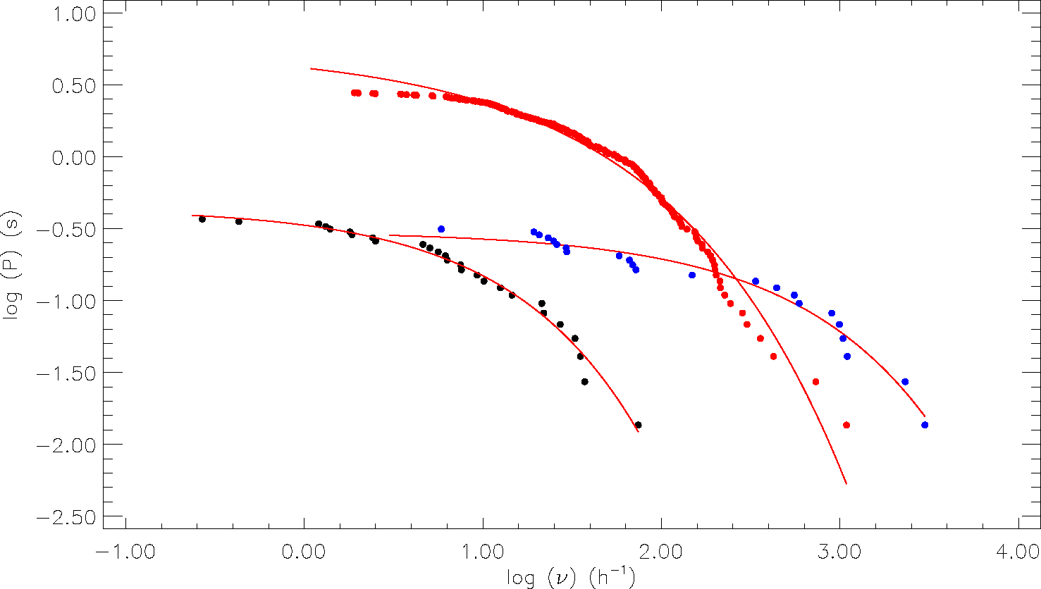
Fig. 10 Cumulative flare frequencies and their models derived for Group 1 (over 27 flares), Group 2 (over 205 flares) and Group 3 (over 23 flares) obtained from V461 Lyr observations. The black circles in the figure represent Group 1, the red ones represent Group 2, the blue circles represent Group 3. In the figure, the red lines represent the exponential distribution models. The color figure can be viewed online.
V1130 Cyg has been observed over 23810.584 h in total. The sum of equivalent duration for its 94 flares has been calculated as 267.576 seconds. V461 Lyr has been observed along 3580.667 h in total. The sum of equivalent durations has been calculated as 25831.721 seconds over its 255 flares. Ishida et al. (1991) has defined two different flare frequencies for the flare activity. These frequencies are expressed by equations 5, 6:
Here,
TABLE 5 FLARE FREQUENCIES COMPUTED FOR BOTH SYSTEMS
| Parameters | All | Group 1 | Group 2 | Group 3 |
|---|---|---|---|---|
| V461 Lyr | ||||
| Total Observation
Time |
3580.667 | 3580.667 | 3580.667 | 3580.667 |
| Flare Number | 255 | 27 | 205 | 23 |
| Total Equ. Dur. |
25831.721 | 352.662 | 13572.733 | 11865.771 |
|
|
0.07122 | 0.00754 | 0.05725 | 0.00642 |
|
|
0.00024 | 0.00003 | 0.00105 | 0.00092 |
| V1130 Cyg | ||||
| Total Observation
Time |
23810.584 | 23810.584 | 23810.584 | - |
| Flare Number | 94 | 30 | 64 | - |
| Total Equ. Dur. |
267.576 | 133.788 | 128.561 | - |
|
|
0.00395 | 0.00126 | 0.00269 | - |
|
|
0.00001 | 0.00001 | 0.00001 | - |
It is well-known that the flare events are generally random phenomena in the case of UV Ceti type flare stars. To test this situation for both targets, we calculated the phase distribution of the flares, depending on the orbital periods of the targets. The total flare numbers were computed in phase intervals of 0.05 for the flares of both targets. Then, we plotted these numbers versus the phase, as seen in Figure 11. We show separately the phase distributions of the flares for each group in the middle and bottom panels of the same figure.

Fig. 11 The distributions of flare total number in each phase interval of 0.05, plotted versus phase for 255 flares detected for V461 Lyr and for 94 flares for V1130 Cyg. In the upper panel the flare phase distributions are shown by a blue line for V461 Lyr and a red line for V1130 Cyg. In the middle and bottom panels, the black lines represent Group 1 flares for both targets, while the red lines show Group 2 flares. In the middle panel, the blue line represents Group 3 flares of V461 Lyr. The color figure can be viewed online.
3. Results and Discussion
Analysis of V1130 Cyg and V461 Lyr data taken from the Kepler Database (Slawson et al. 2011; Matijevič et al. 2012) shows that both systems have highlevel chromospheric activity. It is necessary to investigate which components exhibit chromospheric activity in the systems and to determine their activity levels in comparison with similar stars. For this aim, first of all, the physical parameters of the components have to be determined. For both systems, it is seen that various calibrations and approaches to reveal the physical structure of components have been made in the literature, but no complete light curve analysis has been found. Considering the available radial velocity variations of the targets as shown in Figure 2, both targets should be binary stars. As described in § 2, the semi-amplitudes (K1) of the radial velocities have been estimated as at least 39.19 kms−1 for V1130 Cyg and 117.79 kms−1 for V461 Lyr. These values seem to be enough to support the fact that both targets are the combinations of two stars at least, and not single stars with a planetary system. Therefore, for the first time in the literature, the light curve analyses of the systems have been performed with PHOEBE V.0.32 software, and the parameters obtained in these analyses are listed in Table 2.
The spectral type of V1130 Cyg is given in the literature as F7 + K0 IV (Svechnikov & Kuznetsova 1990). The
temperatures of the components are given as T
1 = 5587 K and T
2 = 6621 K (Armstrong et al. 2014).
In the light curve analysis with PHOEBE V.0.32 software, the temperature of the
primary component has been taken as 6530 K and that of the secondary as 3891±50 K.
The mass ratio (q) of the components has been found to
be0.689±0.001, while the orbital inclination angle (i) of the
system has been obtained as 90◦.00±0◦.01. The mass of the
primary component has been found as 1.337
The spectral type of V461 Lyr’s primary component has been given as G9 (Qian et al. 2018). In the light curve analysis
with PHOEBE V.0.32 software, the temperature of the primary component has been taken
as 5774 K, and that of the secondary as 4206±50 K. The mass ratio
(q) has been found to be 0.999±0.001, while the orbital
inclination angle (i) of the system has been obtained as
89◦.58±0◦.01. The mass of the primary component has been
found to be 0.993
3249 minima times have been computed from V1130 Cyg’s long cadence data and 220 ones from the short cadence data. 716 minima times have been calculated from V461 Lyr’s long cadence data and 75 ones from the short cadence data. The (O−C) II residuals shown in Figure 3 have been obtained by applying a linear correction given by equations 1, 2. It is seen that the expected results have been found, according to both Tran et al. (2013) and Balaji et al. (2015), whose studies were concentrated on the magnetic activity effects on the minima times. The primary and secondary minima times are differentiated by the effect of the chromospheric activity of the systems. If one examines the minima times of V461 Lyr, it will be seen that the chromospheric activity mostly affects the variations of the secondary minima. Therefore, the (O−C) analysis is quite difficult for this target. As seen from the (O − C) II residuals shown in the bottom panel of Figure 3, the correction rates have been found to be remarkably different, analysing the primary minima and the secondary minima together. This makes it difficult to understand the nature of the system. At this point, it cannot be said for sure whether the linear trend seen in the primary minima times is caused by an inadequate analysis, or not. It is possible that it can be a small part of a sinusoidal variation due to the effect of cool spots.
V1130 Cyg has been observed over 23810.584 h in total, according to the available data in the Kepler Database, where 94 flares have been obtained in total. When the distribution of flare equivalent durations versus the flare total times on the logarithmic scales was analysed, an interesting fact was noticed. The obtained OPEA model exhibits two different distributions. The flares were divided into two groups: 30 flares in the first group and 64 flares in the second group. Therefore, two separate OPEA models were derived for both groups. When the parameters of the obtained models have been compared with each other, the statistical tests have shown that these two groups are separate and cannot be modelled under a single model. The Plateau values obtained separately from these two groups have been found to be 2.1997 s for Group 1 and 1.0068 s for Group 2. It is seen that there is approximately a two-times difference between these two Plateau values. The situation was encountered for the first time by Kamil & Dal (2017). Considering that the OPEA models derived by the flares come from different components, the temperatures of the components of V1130 Cyg are suitable to exhibit different group flares, according to Dal & Evren (2011).
V461 Lyr was observed over 3580.667 h in total. As a result of the analysis, 255 flares were obtained in total. Then, the OPEA model was derived for these flares. The same interesting situation was also seen in the case of V461 Lyr. The data cannot be represented by one model. The data seem to be best represented by three different models, shown in Figure 8. Therefore, the flares obtained from V461 Lyr were divided into three groups: 27 flares in the first group, 205 flares in the second group, and 23 ones in the third group. Three OPEA models were created for the flares of these groups. The Plateau values were obtained as 1.9015 s for Group 1, 2.7943 s for Group 2, and 3.4324 s for Group 3. The components’ temperatures could explain the division into two flare groups. In this case, the systems must have an unseen third component to provide a third group. But there has been no observational information about the third body. Besides, there were no background and foreground stars near the system that could exhibit flare activity to create a third group.
Taking into account the frequency definitions of Gershberg (1972), in the case of V1130 Cyg, the flare frequencies of Group 1 were found to be N 1 = 0.00126h−1 and N 2 = 0.00001, while N 1 = 0.00269h−1 and N 2 = 0.00001 for Group 2 flares. From V461 Lyr’s flares, the flare frequencies were found as N 1 = 0.00754h−1 and N 2 = 0.00003 for Group 1 flares, N 1 = 0.05725h−1 and N 2 = 0.00105 for Group 2 flares, and also N 1 = 0.00642h−1 and N 2 = 0.00092 for Group 3. In the case of UV Ceti type single stars, the N 1 flare frequency was found to be N 1 = 1.331h−1 for AD Leo, N 1 = 1.056h−1 for EV Lac. The N 2 flare frequency was found to be N 2 = 0.088 for EQ Peg, N 2 = 0.086 for AD Leo (Dal & Evren 2011). In the case of eclipsing binaries, with just one component being a chromospherically active star, the flare frequencies have been found to be N 1 = 0.01735h−1 and N 2 = 0.00001 for KIC 9641031, N 1 = 0.01351h−1 and N 2 = 0.00006 for KIC 9761199, N 1 = 0.05087h−1 and N 2 = 0.0005 for KIC 11548140 (Yolda¸s & Dal 2016, 2017b,a). As an indicator of flare activity level, one of the most reliable parameters should be the flare frequency if it was determined over long observing durations. In this study, the flare frequencies were computed over 29630.74161 hours, while they were also computed over long observing durations in the cited studies. Consequently, in this study, the flare frequencies are quite suitable to discuss stellar activity levels.
Solving the OPEA models, the Half-life parameter for V1130 Cyg was found to be 1456.515 s for Group 1 flares, 1226.070 s for Group 2 flares. In the case of V461 Lyr, it was found to be 15004.2 s for Group 1, 16767.6 s for Group 2, and 10118.6 for Group 3 s. These values are remarkably higher than the values obtained from classical UV Ceti type stars. For example, they are 433.10 s for DO Cep, 334.30 s for EQ Peg, and 226.30 s for V1005 Ori (Dal & Evren 2011). Similarly, they are 2291.7 s for KIC 9641031, 1014 s for KIC 9761199, 2233.6 s for KIC 11548140 (Yolda¸s & Dal 2016, 2017b,a).
The longest rise time (T r ) was found to be 1706.558976 s for Group 1 and 2765.821248 s for Group 2 in the case of V1130 Cyg. The longest rise time was found to be 1765.447488 s for Group 1, 38840.757120 s for Group 2, and 10592.6832 s for Group 3 in the case V461 Lyr. According to some examples from the classical single UV Ceti type stars, the maximum rise times were 2062 s for V1005 Ori, 1967 s for CR Dra (Dal & Evren 2011). It was found to be 1118.099 s for KIC 9761199 (Yolda¸s & Dal 2017b), while it was 3942.749 s for KIC 11548140 (Yolda¸s & Dal 2017a). In the case of the flares observed in the UV Ceti type single stars, the maximum flare total time was found to be 5236 s for V1005 Ori, and it was 4955 s for CR Dra (Dal & Evren 2011). However, the longest flares obtained in the case of V1130 Cyg were 3413.250144 s for Group 1 and 7885.51805 s for Group 2. The longest flares obtained in the case of V461 Lyr were 58258.0624 s for Group 1, 192431.8967 s for Group 2, and 86506.9597 s for Group 3. The longest flares lasted 5178.87 s for KIC 9641031, 1118.099 s for KIC 9761199 and 22185.361 s for KIC 11548140 (Yolda¸s & Dal 2016, 2017b,a). The comparisons show that V1130 Cyg and V461 Lyr have relatively higher chromospheric activity compared to similar systems, although the values are not as high as those obtained in the case of UV Ceti type single stars.
It has been understood from the variations at out-of-eclipses that the systems exhibit cool spot activity as well as flare activity. The reason for these variations is the rapid evolution of stellar cool spots on the stellar surface. The stellar spot activities seen on the chromospherically active components have been analysed by examining the minima phase variations of the sinusoidal variations versus time. As a result of the analysis, it is seen that the active component of V1130 Cyg has a spot migration with a period of 0.33388 years. However, V461 Lyr has four spots on its two active components. The migration periods were found to be 11.58 years and 10.59 years for two spots on the same component. The migration periods of the other two spots on the other component were found to be 11.81 years and 12.84 years.
The observations of the spot groups on the solar surface show that two permanent active longitudes occur between 180 degrees. These effective longitudes are known as Carrington Coordinates and are fixed structures for some authors, while others indicate that the effective longitude rotation speeds are not constant and may be different (Lopez Arroyo 1961; Stanek 1972). Similarly, stellar cool spots detected on the active components of the systems showed migration, but the migration periods were different for each spot. As shown in the lower panels of Figures 5 and 6, some wave-like variations remain after correcting for migration movements with some linear model fits. From the spots seen for the first time to the end of the observation season in the data, it is seen that the migration periods have a great variation, which reveals that differential rotation on the surfaces of the stars is very strong.
Apart from this situation, as shown in Figure 6, there are two pairs of active longitudes on V461 Lyr, and the active longitudes in each pair are located with a longitude interval of 180 degrees. This means that there are four active longitudes positioned with a longitude interval of 90 degrees. According to this scene, an observer can detect some flares from the longitudes at 90 degrees on the stellar surface. In this case, we expect to see an almost homogeneous phase distribution for the flares from V461 Lyr. On the other hand, as shown in Figure 11, the total number of flares detected in each phase interval of 0.05 is increasing toward the phases of 0.35 and 0.65. It seems that the flare numbers start to increase from phase 0.35 and decrease until phase 0.65. However, the flare number drops to nearly zero at phase of 0.50. The active component should be blacked out by the other component in the direction of the observer. Consequently, according to this scenario, the flare frequency varies from one phase interval to the next one; and it reaches a maximum around phase 0.50, where the stellar surface part is positioned toward the other component. Because of the tidal effect, the possibility of flare occurrence on the surface part facing the other components becomes higher than anywhere on the surface, though the flares can occur anywhere on the stellar surface due to the spotted regions in the active longitude.
In the case of V1130 Cyg, the target has just one active longitude where the cool spots occur. As shown in Figure 11, the flare numbers increase at phases 0.20, 0.35, 0.70, and 0.90. Similarly, the flare number decrease to near zero at phase 0.50. This could be caused by the eclipses of the components. V1130 Cyg exhibits a different behaviour from V461 Lyr. The target shows a nearly homogeneous phase distribution for the flares despite the single active longitude.
In the literature there are several studies such as Hawley et al. (2014); Dal & Özdarcan (2018), in which flare frequency variation versus rotational phase is mentioned. Dal & Özdarcan (2018) demon- strated that the flare frequency of KIC 12418816 increases toward phase 0.85. However, Hawley et al. (2014) indicated that the flare frequency of GJ 1243 does not exhibit any clear variation with phase. At this point, it must be noted that GJ 1243 is remarkably one of the most active stars. Indeed, V1130 Cyg exhibits 94 flares over 29630.742 hours of observing patrol, while V461 Lyr exhibits 255 flares in total. However, Davenport et al. (2014) detected over 6100 individual flare events from GJ 1243 in 7665.6 hours (about 11 months). GJ 1243 is a single M dwarf, most probably a fully convective star; and its whole surface must be fully covered with magnetic lines. As a result, as in the case of UV Ceti type flare stars, the flare time distribution does not exhibit any correlation with the rotation period in the case of GJ 1243, unlike both V461 Lyr and V1130 Cyg.
Apart from the phase distributions of total flare numbers in each phase interval of 0.05, we also examined the phase distributions of each flare group for both systems. One expects that the flares in each group come from different sources due to the different mechanisms working on the stellar surfaces. In this case, it is expected that the flare phase distributions should be maximum around the different phases. However, the distributions shown in Figure 11 indicate that all groups have a maximum around the same phases. This reveals that even if the sources or the mechanisms of each flare group are different from each other, the locations of each flare group on the stellar surface are roughly the same.

