


 nueva página del texto (beta)
 Inglés (pdf)
 Artículo en XML
 Referencias del artículo
 Enviar artículo por email
 Citado por SciELO
  Similares en
SciELO
Similares en
SciELO 
 Permalink
1. INTRODUCTION
The study of δ Scuti stars has undergone many changes since its inception. Soon after the pioneering works of Eggen (1957) and Millis (1966, 1968), systematic studies like those of Breger (1979) and the early considerations about the nature of their variability by the French group led by Le Contel et al. (1974), as well as the later coordinated longitudinal campaigns designed to discover the true nature of the pulsational variability, altered the nature of our knowledge of these stars. During these years some researchers such as Zessewitch (1950) and Abhyankar (1959), among others, recognized the value of using the old data sets which provided, as in the present study, time bases of fifty years or more leading to more precise interpretations of the variability. However, the attainable limits of ground-based observations were finally reached and efforts were made to study these variables from space.
As Garrido and Poretti (2004) pointed out, teams dedicated to δ Scuti stars have begun changing their observational strategies. After the Canadian satellite MOST was successfully launched to study asteroseismology from space, other missions were designed to determine adequate frequency resolutions. This satellite, and COROT, were the first to study δ Scuti stars from space. CoRoT (Convection, Rotations, and Planetary Transits), led by the CNES in association with French laboratories with large international participation, was a satellite built to study the internal structure of stars and to detect extrasolar planets. It continuously observed star fields in the Milky Way for periods of up to 6 months. Over the course of 2,729 days, CoRoT collected some 160,000 light curves showing variations of star brightness over time. This mission ended in June 2014.
There have been several other space projects. One of the most important was that of NASA’s Kepler satellite, which was launched on March 6, 2009 with the primary mission of searching for exoplanets via planetary transits using high-precision, long time-series CCD photometry with a secondary mission of studying stellar variability (Guzik et al., 2019). In 2013 the K2 mission was developed to observe 19 new fields along the ecliptic plane. δ Scuti variables have been included in these campaigns since they are a promising type of star for research using pulsations to infer interior structure and, as a result, to test the input of physics and methods of solar and stellar modelling. Multiple papers have utilized the Kepler data, and as Guzik et al. (2019) pointed out, the lists of candidate stars observed for these data could be used to discover targets for asteroseismic research.
Recent studies of δ Scuti stars using data from the Kepler mission include Bowman and Kurtz (2018) who demonstrated that an ensemble-based approach using space photometry from the Kepler mission was not only possible, but it was also valuable as a method to identify stars for mode identification and asteroseismic modelling. This work was extended by Antoci et al. (2019) for hot young δ Scuti stars which were missing in the Kepler mission data set.
Kepler’s database, combined with other satellite results such as Gaia DR2 that provided the parallaxes, has served to derive precise luminosities (Murphy et al., 2019) for stars in and around the δ Scuti instability strip for a sample of over 15 000 A and F stars with δ and non δ Sctuti stars. Murphy et al., (2019) determined a new empirical instability strip based on the observed pulsator fraction that is systematically hotter than the theoretical strips. Ziaali et al. (2019) examined the period-luminosity (P-L) relation for δ Sctuti stars with the same Gaia DR2 parallaxes for the sample of Rodriguez et al. (2000) as well as 1124 stars observed by the Kepler mission and determined absolute magnitudes. Barcelo Forteza et al. (2020) remarked that thanks to the high-precision photometric data legacy from space telescopes, like CoRoT and Kepler, the scientific community was able to detect and characterize the power spectra of hundreds of thousands of stars. Thanks to long-duration high-cadence TESS light curves, they could analyze more than two thousand δ Scuti classical pulsators and proposed the frequency at maximum power as a proper seismic index, since it is directly related to the intrinsic temperature, mass and radius of the star.
Extending the study of large satellite data sets, Jayasinghe et al. (2020) characterized an all-sky catalogue of 8400 δ Scuti variables in ASAS-SN, which included 3300 new discoveries and combined with the Gaia DR2 derived period-luminosity relationships for both the fundamental mode and overtone pulsators. The determined results are indicative of a Galactocentric radial metallicity gradient. In their sample, Jayasinghe et al. (2020) identified two new δ Scuti eclipsing binaries, ASASSN-V J071855.62434247.3 and ASASSN-V J170344.20-615941.2 with short orbital periods of 2.6096 and 2.5347 d, respectively. Regarding particular stars, Handler et al. (2020) carried out a study of a close binary system, HD 74423, discovered by TESS. They claim that it might be the prototype of a new class of obliquely pulsating stars in which the interactions of stellar pulsations and tidal distortion can be studied.
In the present paper we utilize both the observations of the AD CMi star obtained decades ago to determine its secular behavior as well as uvby−β to determine its physical parameters. The HADS star AD CMi has the following characteristics: right ascension and declination of 07:52:47.18, +01:35:50.50 (epoch 2000), magnitude of 9.38, a spectral type of F0IV, a period of 0.12297443d (2.9 hr) and an amplitude of variation of 0.3mag. All these features make it an easy target for the small telescopes provided with CCD cameras that are used in our astronomical courses.
With respect to the background of the star, according to Anderson and McNamara (1960) AD CMi was discovered by Hoffmeister (1934) and Zessewitch (1950) who described it as an eclipsing variable of
Algol type, with a period of
The last comprehensive study of AD CMi was done by Khokhuntod et al. (2007). With observations carried out in 2005 and 2006, they analyzed the pulsation of the star with the derived multiple frequencies fitted to their data. Besides the dominant frequency and its harmonics, one low frequency (2.27402c/d) was discovered which, they stated, provided a reasonable interpretation for the long-noticed luminosity variation at maximum and minimum light. The results provided the updated value of period of 0.122974478d, and seemed to support the model of a combination of the evolutionary effect and light-time effect of a binary system. Now, with an extended time basis of more than twelve years we can verify and refine their findings.
In order to carry out an analysis to determine the physical parameters, uvby−β photoelectric photometry can be considered. These include several sources starting with the observations of Epstein & Abraham de Epstein (1973), Rodríguez (1988) and the observations presented in this paper carried out in 2013, 2014, 2016, 2017, 2018 and 2019, and summarized in Table 1.
TABLE 1 LOG OF OBSERVING SEASONS AND NEW TIMES OF MAXIMA OF AD CMI
| Date | Observers/reducers | Npoints | Time span | Nmax | Tmax | Telescope | Filters | Camera | Observatory |
|---|---|---|---|---|---|---|---|---|---|
| yr/mo/day | (day) | 2400000+ | |||||||
| 13/02/0910 | cvr/cvr | 202 | 0.13 | 1 | 56333.8206 | m1 | G | ST8 | TNT |
| 13/02/2223 | aas/arl | 226 | 0.12 | 1 | 56346.7301 | m1 | wo | ST8 | TNT |
| 13/11/1718 | cvr/jhp | 20 | 0.09 | 1 | 56613.9390 | 84 | uvby − β | spectr | SPM |
| 14/04/0506 | AOA14/cgs | 99 | 0.08 | 1 | 56753.6540 | m2 | wo | ST8300 | TNT |
| 16/01/1213 | aas,jg/jhp | 48 | 0.01 | 1 | 57400.8690 | 84 | uvby − β | spectr | SPM |
| 16/01/2122 | ESAOBELA16/cgs | 148 | 0.20 | 1 | 57409.8501 | m1 | G | ST8 | TNT |
| 16/01/2122 | ESAOBELA16/cgs | 179 | 0.15 | 1 | 57409.8501 | m2 | V | 1001 | TNT |
| 16/01/2223 | ESAOBELA16/dsp | 112 | 0.16 | 0 | m2 | V | ST8 | TNT | |
| 16/02/1112 | dsp/dsp | 130 | 0.14 | 1 | 57430.7541 | m2 | V | 1001 | TNT |
| 16/02/1213 | AOA16/dsp | 80 | 0.06 | 0 | me | V | 1001 | TNT | |
| 16/03/1112 | AOA16/dsp | 167 | 0.15 | 1 | 57459.6543 | m1 | V | 1001 | TNT |
| 16/03/1213 | AOA16/dsp | 103 | 0.12 | 0 | m1 | V | 1001 | TNT | |
| 16/12/1314 | dsp/dsp | 42 | 0.11 | 0 | 84 | uvby − β | spectr | SPM | |
| 17/01/1415 | ESAOBELA17/dsp | 144 | 0.12 | 1 | 57768.8131 | m1 | V | 1001 | TNT |
| 18/01/1112 | ESAOBELA18/dsp | 80 | 0.09 | 0 | me | V | 1001 | TNT | |
| 18/01/1213 | ESAOBELA18/dsp | 133 | 0.07 | 0 | me | V | 1001 | TNT | |
| 18/01/2122 | ESAOBELA18/dsp | 137 | 0.12 | 0 | me | V | 1001 | TNT | |
| 18/03/0304 | AOA18/dsp | 157 | 0.15 | 1 | 58181.7596 | m1 | V | 1001 | TNT |
| 18/03/1718 | AOA18/dsp | 129 | 0.13 | 1 | 58195.7759 | m1 | V | 1001 | TNT |
| 19/01/1516 | ESAOBELA19/hh | 97 | 0.15 | 1 | 58499.8951 | m2 | V | ST8 | TNT |
| 19/01/1819 | ESAOBELA19/hh | 205 | 0.16 | 1 | 58502.8419 | m2 | V | ST8 | TNT |
| 19/01/2122 | ESAOBELA19/hh | 141 | 0.19 | 1 | 58505.9170 | m2 | V | ST8 | TNT |
| 19/01/2223 | ESAOBELA19/hh | 186 | 0.21 | 2 | 58506.7780 | m2 | V | ST8 | TNT |
| 58506.9044 | |||||||||
| 19/02/0102 | jgt/jgt | 228 | 0.27 | 2 | 58516.7387 | m2 | wo | 8300 | TNT |
| 58516.8638 | |||||||||
| 19/03/0102 | AOA19/arl | 47 | 0.04 | 0 | m1 | V | 1001 | TNT | |
| 19/03/1516 | AOA19/arl | 32 | 0.02 | 0 | me | V | 1001 | TNT | |
| 19/03/1617 | AOA19/arl | 187 | 0.14 | 1 | 58559.7805 | me | V | 1001 | TNT |
Notes: jhp, J. H. Peña; dsp, D. S. Piña; arl, A. Rentería; jgt, J. Guillén; cvr, C. Villarreal; cgs: C. García; hh, H. Huepa AOA14: N. Ordoñez, S. Mafla, W. Fajardo, M. Rojas, I. Cruz, O. Martinez, E. Rojas, J. Rosales, W. Fajardo, A. Garcia & W. Fuentes; ESAOBELA16: A. Rodríguez, V. Valera, A. Escobar, M. Agudelo, A.Osorto, J. Aguilar, R. Arango, C. Rojas, J. Gómez, J. Osorio, & M. Chacón,; AOA16: Juarez, K. Lozano, K., Padilla, A., Santillan, P. and Velazquez R., ESAOBELA17: Ramirez, C., Rodriguez, M, Vargas, S., Castellon, C., Salgado, R., Mata, J., de la Fuente, D., Santa Cruz, R., Gonzalez, L., Chipana, K.; ESAOBELA18: Calle, C., Huanca, E., Uchima, J., Ramírez, R., Funes, R., Martinez, J., Mejía, R., Sarmiento, Y., Cruz, M., Meza, E., Alvarado, N., Huaman, V. & Ochoa, G.; AOA18: A. L. Zuñiga, J. L. Carrillo, S. B. Juárez, B. Chávez & D. Navez; ESAOBELA19: A. Belen Blanco, T. Benadalid, J. M. Donaire, M. Quiroz-Rojas, P. Escobar, M. Mireles, R. Mejía, A. León, C. Zelada, J. Ng, A. Arcila, L. E. Salazar, P. Escobar & M. M. Mireles; AOA19: I. Soberanes, H. Posadas, C. Castro, J. Briones & M. Romero.
2. OBSERVATIONS
Although some of the times of maximum light of this star have been reported elsewhere (Peña et al., 2017), we here present new times of maxima and the detailed procedure followed to acquire the data. The observations were done at both the Observatorio Astronómico Nacional of San Pedro Mártir (SPM) and that of Tonantzintla (TNT), in México. Table 1 presents the log of observations, as well as the new times of maximum light.
2.1. Data Acquisition and Reduction at Tonantzintla
Three 10-inch Meade telescopes were utilized at the TNT Observatory and are denoted by m1, m2 and me. These telescopes were equipped with CCD cameras and the observations were done using V and G filters. During all the observational nights this procedure was followed: the integration time was 1 min and there were around 11,000 counts, enough to secure high precision. The reduction work was done with AstroImageJ (Collins & Kielkopf (2012)). This software is relatively easy to use and, besides being free, it works satisfactorily on the most common computing platforms. With the CCD photometry two reference stars were utilized whenever possible in a differential photometry mode. The results were obtained from the difference Vvariable −Vreference and the scatter calculated from the difference V reference1− V reference2. Light curves were also obtained. In order to calculate the times of maximum light a program that considers the derivative function was used. A fifth polynomial was adjusted between the selected points in order to enclose the point of maximum light. On applying the derivative, as a criterion, the roots were determined in such a way that an f adjustment function was found, so that in the open selected interval, the derivative equal to zero was a minimum (if it was convex) or maximum (if it was concave) relative to f. The new times of maximum light are listed in Table 1. In this table, in Column 1 the date of observation is listed, in Column 2 the observers/reducers; in Column 3 the obtained number of points during the night, and in Column 4 the time span of the observations. Column 5 specifies the number of maxima for that night; Column 6 the time of maximum in HJD-2400000; and Column 7 the telescope utilized (m1, m2 and me stand for small 10” Meade telescopes, whereas 84 describes the telescope at the SPM observatory); Column 8 describes the filter utilized (V in the UBV system and G for the GRB filter system, whereas in the uvby−β we utilized only the y filter transformed into Olsen’s (1983) photoelectric photometry system. Finally, the last two Columns 9 and 10 specify the CCD camera and the observatories, Tonantzintla (TNT) and San Pedro Mártir (SPM).
2.2. Data Acquisition and Reduction at SPM
As was stated in Peña et al. (2016) reporting on BO Lyn, the observational pattern as well as the reduction procedure have been employed at the SPM Observatory since 1986 and, hence, have been described many times. A detailed description of the methodology can be found in Peña et al. (2007).
The star AD CMi was observed in uvby −β photometry over various seasons: November, 2013; January, December, 2016 and 2017. The first one covered six nights, whereas the second one three nights in January and seven in December, 2016. AD CMi was observed on only one night in the 2017 December season.
Over the nights of observation of the AD CMi star the following procedure was used: Each measurement consisted of at least five ten-second integrations of the star and three ten-second integrations of the sky simultaneously for the uvby filters, and almost simultaneously for the narrow and wide filters that define Hβ.
The details of the second season are described in Peña et al. (2019), whereas for the 2013 season the transformation coefficients of that night are listed in Table 2. In the 2016 season three nights were lost due to bad weather.
TABLE 2 MEAN VALUES AND STANDARD DEVIATIONS < σ > OF THE TRANSFORMATION COEFFICIENTS OBTAINED FOR THE SEASONS
| Season | B | D | F | J | H | I | L |
|---|---|---|---|---|---|---|---|
| 2013 Nov | 0.027 | 0.973 | 1.034 | 0.034 | 1.022 | 0.146 | -1.495 |
| < σ > | 0.029 | 0.010 | 0.004 | 0.014 | 0.031 | 0.028 | 0.015 |
| 2016 Jan | 0.031 | 1.008 | 1.031 | -0.004 | 1.015 | 0.159 | -1.362 |
| < σ > | 0.028 | 0.003 | 0.015 | 0.015 | 0.005 | 0.004 | 0.060 |
| 2016 Dec | 0.134 | 0.993 | 1.024 | 0.043 | 1.025 | 0.101 | |
| < σ > | 0.243 | 0.009 | 0.065 | 0.055 | 0.009 | 0.026 | |
| 2017 Dec | 0.016 | 1.013 | 1.002 | 0.023 | 1.032 | 0.131 | -1.314 |
| < σ > | 0.084 | 0.047 | 0.040 | 0.035 | 0.015 | 0.029 | 0.100 |
What must be emphasized here are the transformation coefficients for the observed seasons (Table 2) and the season errors which were evaluated using the observed standard stars. These uncertainties were calculated through the differences in magnitude and colors for (V , b−y, m 1, c 1 and Hβ) which are (0.0870,
0.0065, 0.0085, 0.0212, 0.0179); (0.054, 0.012, 0.019, 0.025, 0.012) and (0.032, 0.010,0.011,0.013, 0.012) for the 2013 and both the 2016 and 2017 seasons, respectively, for a total of 94 points in uvby and 68 points in Hβ, which provide a numerical evaluation of our uncertainties. We must call attention to the bad quality of the December 2016 season. However, since the effects of the clouds compensate each other, the color indexes gave reasonable values, whereas the V showed significant larger scatter and, will not be taken into account. The obtained data will be sent to the archives and are available upon request.
3. PERIOD DETERMINATION
To determine the period behavior of AD CMi the following three methods were employed: (1) Time series analyses of different data sets. (2) Period determination through O−C differences minimization (PDDM), and (3) O−C differences calculated utilizing a compiled collection of times of maximum light.
The previously determined ephemerides equations, as well as the newly determined ones are listed in Table 3.
TABLE 3 LOG OF EFEMERIDES EQUATIONS
| Reference | T0 | Period | A | β |
|---|---|---|---|---|
| Anderson60 | 2436601.8228 | 0.122974 | ||
| Breger75 | 2442429.4582 | 0.12297443 | ||
| Rodriguez88 | 2436601.8226 | 0.12297431 | 1.9 × 10⁻¹² | |
| Rodriguez90 | 2436601.8225 | 0.12297426 | 2.7 × 10⁻¹² | |
| Yang92 | 2436601.8224 | 0.12297429 | 2.19 × 10⁻¹² | |
| Burchi93 | 2447506.5815 | 0.122974448 | ||
| Kim94 | 2442429.4582 | 0.12297455 | ||
| Fu96 | 2436601.8203 | 0.12297446 | 4.6 × 10⁻¹³ | |
| Fu2000 | 2436601.8203 | 0.122974463 | 3.50 × 10⁻¹³ | |
| Hurta2007 | 2436601.82736 | 0.12297451 | ||
| Pongsak2007 | 2436601.8219 | 0.122974478 | ||
| PP time series | 2436601.8186 | 0.122974518 | ||
| PP PDDM | 2458559.7805 | 0.122974511 |
3.1. Time Series
As a first method to determine the period, we used a time series method which is commonly utilized in the δ Scuti star community: Period04 (Lenz & Breger, 2005). There are several data sets which can be analyzed with this code:
i) The combined data in uvby − β of Rodriguez et al. (1988) and the present paper’s data.
In this case, we were fortunate enough that AD CMi had been observed in 1984 by Rodriguez et al. (1988) with a spectrophotometer similar to that of the SPM observatory, so a time series analysis was possible using their data along with the observations reported in the present paper. The initial time is HJD 2445766.3497 and the end time HJD 2457400.9452, with a total of 339 data points. The time span covered is then 11634.5955d or 31.8yr which is 94684 cycles, an enormous gap during which no observations were made of this system. To combine both seasons we first had to level them. Rodriguez et al. (1988) published their result in differential magnitudes relative to the BD + 2◦1804 star. We observed this star both in 2017 (once) and 2018 (three times) and found that its photometric values were 8.181 ± 0.010 in V ; 0.335 ± 0.003 in (b − y); 0.155 ± 0.005 in m 1 and 0.347 ± 0.006 for c 1. The uncertainties are the standard deviation of the four measurements. The details of the accuracy of each season can be found in Peña et al. (2019). The analysis of these data gave the results listed in Table 4 (Set 1), with a zero point of 8.6046, and residuals of 0.014532.
ii) To this data set we added that of Epstein &Abraham de Epstein (1973) (Set 2). They observed this star in 1973 and considered it to be an RR Lyra star. A few points in each of the four consecutive reported nights comprise the data sample of only fifteen data points. This enlarges the times basis from HJD2441010.6949, their first reported point, to HJD2457400.9452, our last observed point, a difference of 16390d (44.9 yr) equal to 133388 cycles. However, the gaps between the sets are enormous.
iii) To fill these gaps we considered the ASAS data (Pojmanski et al. 2005), because this sample contains 464 points over a time span of 907 days in the years from 2002 to 2005. The V magnitude sample was increased with the values of Dean et al. (1977), Epstein et al. (1973), Balona & Stobie (1983), and Kilambi & Rahman (1993). Therefore, we compiled 1300 points in this final data set. The photometry presented by Kilambi & Rahman (1993) lists differential magnitudes referred to HD 64561 star, with a magnitude of 8.20 ± 0.02.
TABLE 4 OUTPUT OF PERIOD04 CALCULATED WITH THE V MAGNITUDE OF SEVERAL DATA SETS
| Considered data | Nr. | Frequency | Amplitude | Phase | Residuals |
|---|---|---|---|---|---|
| Set 1 | F1 | 8.13821236 | 0.145219814 | 0.2134 | 0.0281 |
| F2 | 16.2544156 | 0.0281107579 | 0.2715 | 0.0199 | |
| F3 | 0.00249795 | 0.754162399 | 0.9004 | 0.01453 | |
| Set 2 | F1 | 8.13830066 | 0.140946042 | 0.1759 | 0.036 |
| F2 | 16.245476 | 0.0289895308 | 0.4235 | 0.028 | |
| F3 | 0.00256016 | 0.28816242 | 0.1689 | 0.229 | |
| Set 3 | F1 | 8.13176594 | 0.140564142 | 0.0110 | 0.3364 |
| F2 | 16.2635352 | 0.0262466142 | 0.5018 | 0.0282 | |
| F3 | 1.0705324 | 0.0121627692 | 0.4000 | 0.0266 |
Notes: Set 1: Rodriguez et al. (1988) and the present paper’s uvby − β. Set 2: Adds uvby of Epstein and Abraham de Epstein (1973). Set 3: All data listed in Table 3.
The analysis of Period04 is presented in Figure 1. At the top is the periodogram of the original data and at the bottom, that of the residuals after the produced frequency was subtracted. Table 4 summarizes these results (set 3).
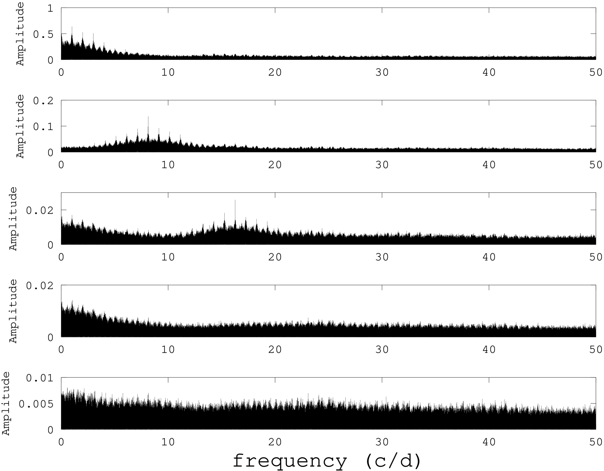
Fig. 1 The analysis of Period04 is presented. Descending, the periodogram of the window function and subsequently each maxima is presented. At the bottom, the residuals after the three frequencies have been subtracted. Emphasis should be made on the Y-axis scale.
The results of utilizing Period04 gave as the first frequency 8.13830066c/d with an amplitude of 0.1409 and a phase of 0.1759. Evaluating the residuals we obtained the following numerical values: 16.254, 0.02898 and 0.4234 respectively. Fitting the data to these values gave as residuals a frequency of 0.0025c/d with an amplitude of 0.2881 and a phase of 0.1689. These values correspond to a period of 0.12287577d for the first frequency and to 0.061523d. Given the numerical frequency values the results of Period04 gave f and 2f, or a value close to it (16.276c/d). When a phasevs.magnitude plot was constructed, the phasing shows the correctness of the determined period (Figure 2).
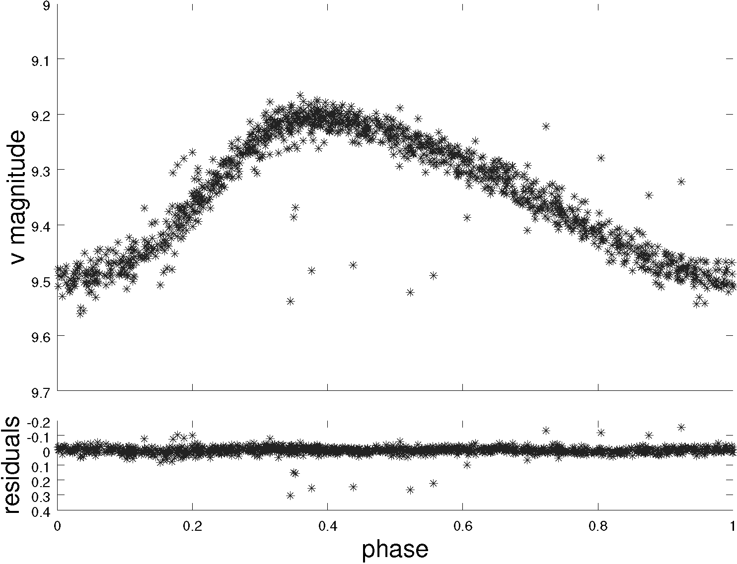
Fig. 2 Top: Phase diagram after the analysis of Period04 using frequency F1 set 3 of Table 4. Bottom: The residuals after the three frequencies have been subtracted.
3.2. Period Determination Through O−C Differences Minimization (PDDM)
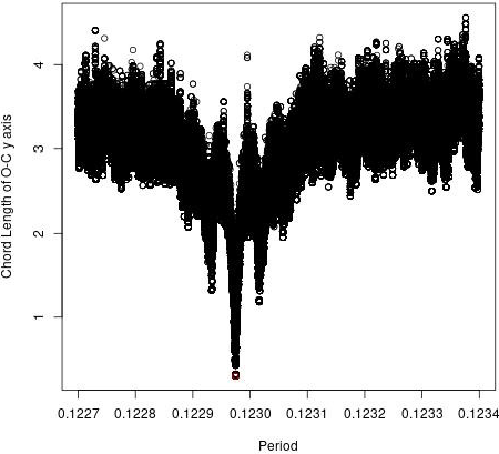
We employed another method based on the concept of the minimization of the chord length linking all the points in the O−C diagram for different values of changing periods, looking for the best period which corresponds to the minimum chord length (see the case of KZ Hya, Peña et al. 2018).
A set of 94 times of maxima was considered for this analysis. Taking this into consideration, we used the determined period value in § 3.1 and the standard deviation of those consecutive differences to keep an interval span in which the period is located; those values are 0.1230±0.0002d. Maintaining a period precision of a billionth and taking the interval span period into consideration, 500,000 periods were used to perform this method. The T 0 used to calculate the O−C diagrams was 2458559.7805. Then the best period is the one with the smallest chord length and it is shown in Figure 3.
The ephemerides equation is then:
As we can see in Figure 4, the plot shows a slope and marginally a sinusoidal behavior which can be related to the light-travel time effect (LTTE), revealing the possible presence of a second body. This visualization is later confirmed (Figure 5).


Then, we adjusted a sinusoidal function to the O−C diagram performing a fit using LevenbergMarquardt Algorithm. We then used a combination of the chord length minimization and the non-linear fit for a sinusoidal function, taking the periods with the minimum chord length and, as a second criterion, the RMS error of the non-linear fitting.
The fitting equation for the O−C diagram is
and the continuous line in Figure 6 shows the sinusoidal fit over the O−C diagram with a new period.
The sinusoidal function parameters are listed in Table 5. Accordingly, the period of the sinusoidal behavior is 10,247.8759 days or 28.1 years.

TABLE 5 EQUATION PARAMETERS FOR THE SINUSOIDAL FIT
| Value | |
|---|---|
| Z |
|
|
|
|
|
|
|
|
|
|
| RSS residuals |
|
The ephemerides equation determined by this method is:
The goodness of the model is determined by the RSS residuals listed in Table 3.
3.3. O−C and Mass Determination
Before calculating the coefficients of the ephemerides equation, we reviewed the existing literature related to AD CMi. Several authors have conducted studies on the O−C behavior of these particular objects and, in this preliminary stage, we took the existing updated list of times of maxima from the literature, plus the data that we acquired. We built the O−C diagram with the obtained period values from Period04 (set 3).
The O−C diagram (Figure 6) shows a variation and a cyclic pattern with no quadratic component. Hence our solution is of the form:
where τ is the equation given by Irvin (1952)
The fit (Figure 6) was done by least squares with the Levenberg-Marquard algorithm, using the relation provided by Li & Qian (2010) in their equation 3:
Where
With
where e, ω, P orb , T, P and E are: the eccentricity, the periastron longitude, the orbital period, the time of periastron passage, the period of pulsation of AD CMi (P = 0.122974518) and the epoch, respectively.
Since equation 5 is trascendental, the solutions for E ∗ are obtained through Bessel series
where
The obtained orbital parameters with the fit are presented in Table 6 and have been used to build the plot of Figure 6.
The mass function is given by Fu et al. (2008) with P orb = 32.33 (yr).
To calculate the mass of the companion, the solution of the following function was evaluated for m 2:
for a mass of
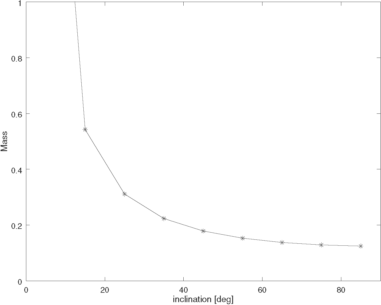
TABLE 7 ORBITAL SEMI-MAJOR AXIS AND COMPANION’S MASS AS A FUNCTION OF ANGLE
|
|
A (AU) |
|
|---|---|---|
| 5 | 8.93975 | 2.30637 |
| 15 | 3.01040 | 0.54239 |
| 25 | 1.84362 | 0.31112 |
| 35 | 1.35840 | 0.22320 |
| 45 | 1.10188 | 0.17854 |
| 55 | 0.95116 | 0.15286 |
| 65 | 0.85969 | 0.13748 |
| 75 | 0.80663 | 0.12863 |
| 85 | 0.78212 | 0.12456 |
Pongsak Khokhuntod et al. (2007) stated that the binary orbit has a period of 27.2 ± 0.5 years, with an eccentricity of 0.8 ± 0.1. However, since there is a big gap between the first 12 data points and the rest, and the bulk of the data spans only one cycle, this result should not be considered to be an accurate solution of the orbital parameters.
However, this is a plausible solution because it diminishes the dispersion, as can be see in the residuals in Figure 6. From the data shown in Table 7 and represented in Figure 7 we can consider the mass determination of the companion as a function of this angle since we cannot determine the inclination angle. If we do so, the probability that the companion is an M type star is 75%. The minimum mass is discarded because in our light curves there is no evidence of eclipses. Of course, more observations are needed to corroborate this result
3.4. Period Determination Conclusions
Despite having been determined to be a variable star many years ago, the nature of this star has been variously described, from a binary star to a pulsating star, as well as an RR Lyrae and, finally a δ Scuti star. Since then, more information has been gathered but no period analysis was done. In the present paper, different approaches were utilized to determine the stability of the pulsation. With respect to its period determination and interpretation, it has varied from a periodic star to a quadratic fit which should be interpreted as a changing period.
The first method used to determine the periodic content utilized a time series analysis of different data sets. The first set is that of the V filter of the photometry of Rodriguez et al. (1988) and that of the V filter of the uvby − β photometry of the present paper. The time span covered for all the data is 17084d or 47 years, which in cycles is 138926. The second method we used was PDDM which gives a first approximation to the period of a binary system. Finally, in the third method we utilized O−C analyses via the LTTE.
The amazing result is that the uvby−β photoelectric photometry adjusts to a phase both in magnitude and color indexes with the properly determined frequency.
In conclusion, there was a systematic improvement of the period, but not only that: Yang et al. (1992) postulated that the quadratic fit was much better, so the period was considered to be increasing at a rate of (1.3 ± 0.07 × 10⁻⁸ days/year) although they could not fit the curve well with the observations from 1985 and 1986.
They suggested that more observations were urgently needed to clarify the true situation of the period variation. It is just now that these observations and analysis have been done with congruent results.
Data from other independent sources, such as the Kepler field or TESS, would have been very useful but, unfortunatelly, the star was not observed by either.
4. PHYSICAL PARAMETERS
Determination of the physical parameters of a star is possible if a comparison of theoretical models, such as those of Lester, Gray & Kurucz (1986), (hereinafter LGK86), is made. The uvby − β unreddened color indexes are used because the uvby − β photometric system has the advantage that reddening and unreddened colors can be determined from the photometry, the proper calibrations depending on the spectral type of the considered object. Nissen’s (1988) procedure is applicable for A and F type stars and Shobbrook’s (1984) for earlier spectral types. Hence, accurate determination of the spectral type is crucial.
According to Houk and Swift (1999) as reported in Simbad, AD CMi has a spectral type of F0IV/V. To corroborate this, we fixed its position in the unreddened color diagram [m 1] vs. [c 1] that was established for the open cluster Alpha Per (Peña et al. 2006) for which the unreddened color indexes were compared to the spectroscopically determined spectral types from several sources. In all cases the photometrically determined spectral types coincided with those determined spectroscopically, assuring us of the goodness of the method. We applied these calibrations to the uvby − β photometry obtained (Table 8) for AD CMi corroborating first that the known spectral type of AD CMi was correct (Figure 8). To further check our results using uvby − β photometry, we calculated the unreddened indexes [m 1] [c 1] from the other two sources, that of Epstein et al. (1973) and of Rodriguez et al. (1988). This latter reference reported the photometry of AD CMi differentially with respect to the star HD 63776 which was measured during two different years 2017 (once) and 2018 (three points) and obtained the following values for V , (b − y)1, m 1, and c 1 (8.181 ± 0.010, 0.335 ± 0.003, 0.155 ± 0.005, 0.347 ± 0.006) respectively which immediately allowed us to calculate the uvby − β values for AD CMi in the 1988 season. In all three cases with uvby − β photometry, the location of AD CMi is in the same position, making its spectral type determination unquestionable. In view of this, the prescription to determine the reddening is that of Nissen (1988).
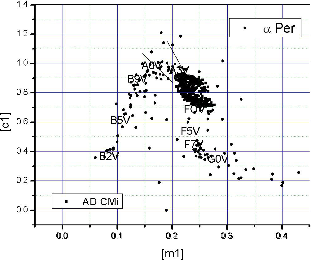
Fig. 8 Position of AD CMi in the unreddened indexes of Alpha Per from all sources with uvby−β photometry.
TABLE 8 AVERAGED MAGNITUDES, COLOR INDEXES AND β WITH THEIR UNCERTAINTIES IN PHASE BINS AS A FUNCTION OF PHASE
| Phase | V | (b − y) | m 1 | c 1 | β | σ V | σ (b − y) | σ m 1 | σ c 1 | σ β | N |
|---|---|---|---|---|---|---|---|---|---|---|---|
| 0.00 | 9.208 | 0.152 | 0.179 | 0.936 | 2.792 | 0.012 | 0.007 | 0.013 | 0.018 | 0.014 | 15 |
| 0.05 | 9.221 | 0.155 | 0.179 | 0.933 | 2.776 | 0.012 | 0.009 | 0.021 | 0.021 | 0.012 | 12 |
| 0.10 | 9.245 | 0.165 | 0.175 | 0.918 | 2.774 | 0.011 | 0.009 | 0.019 | 0.024 | 0.016 | 17 |
| 0.15 | 9.269 | 0.169 | 0.182 | 0.884 | 2.778 | 0.013 | 0.005 | 0.014 | 0.022 | 0.015 | 9 |
| 0.20 | 9.299 | 0.176 | 0.175 | 0.883 | 2.759 | 0.009 | 0.010 | 0.019 | 0.026 | 0.015 | 14 |
| 0.25 | 9.322 | 0.188 | 0.169 | 0.866 | 2.749 | 0.017 | 0.008 | 0.010 | 0.021 | 0.014 | 16 |
| 0.30 | 9.361 | 0.192 | 0.171 | 0.845 | 2.752 | 0.018 | 0.006 | 0.018 | 0.026 | 0.011 | 16 |
| 0.35 | 9.399 | 0.201 | 0.175 | 0.820 | 2.740 | 0.019 | 0.011 | 0.022 | 0.027 | 0.017 | 21 |
| 0.40 | 9.430 | 0.210 | 0.171 | 0.810 | 2.735 | 0.019 | 0.004 | 0.014 | 0.021 | 0.019 | 13 |
| 0.45 | 9.447 | 0.216 | 0.171 | 0.796 | 2.726 | 0.033 | 0.005 | 0.012 | 0.024 | 0.019 | 16 |
| 0.50 | 9.480 | 0.215 | 0.176 | 0.786 | 2.718 | 0.016 | 0.005 | 0.014 | 0.017 | 0.007 | 12 |
| 0.55 | 9.493 | 0.218 | 0.174 | 0.777 | 2.719 | 0.015 | 0.007 | 0.012 | 0.014 | 0.017 | 11 |
| 0.60 | 9.481 | 0.214 | 0.180 | 0.777 | 2.725 | 0.019 | 0.007 | 0.017 | 0.023 | 0.020 | 13 |
| 0.65 | 9.460 | 0.210 | 0.177 | 0.783 | 2.736 | 0.022 | 0.008 | 0.015 | 0.016 | 0.009 | 13 |
| 0.70 | 9.438 | 0.194 | 0.187 | 0.776 | 2.743 | 0.025 | 0.011 | 0.022 | 0.026 | 0.026 | 9 |
| 0.75 | 9.372 | 0.189 | 0.175 | 0.806 | 2.751 | 0.021 | 0.007 | 0.015 | 0.020 | 0.019 | 11 |
| 0.80 | 9.314 | 0.178 | 0.175 | 0.832 | 2.760 | 0.025 | 0.009 | 0.012 | 0.028 | 0.014 | 22 |
| 0.85 | 9.241 | 0.163 | 0.176 | 0.872 | 2.784 | 0.021 | 0.009 | 0.017 | 0.036 | 0.014 | 26 |
| 0.90 | 9.209 | 0.151 | 0.187 | 0.895 | 2.792 | 0.015 | 0.008 | 0.017 | 0.030 | 0.020 | 35 |
| 0.95 | 9.203 | 0.145 | 0.187 | 0.925 | 2.796 | 0.014 | 0.008 | 0.016 | 0.020 | 0.017 | 33 |
We determined the unreddened indexes of AD CMi which were measured over three different seasons at SPM: 2013, 2016 and 2017. The spectral types we determined were A and F, not late enough to calculate the metallicity.
We relied on uvby − β photometry again to determine the metallicity. We followed a prescription proposed by Meakes et al. (1991) for short period Population II Cepheids from uvby − β photometry. LGK86 calculated grids for stellar atmospheres for G, F, A, B and O stars for different values of [Fe/H] (-3.0, -2.5, -2.0, -1.5,-1.0, -0.5, 0.0, 0.5 and 1.0) in a temperature range from 5500 up to 50 000 K. The surface gravities vary approximately from the main sequence values to the limit of the radiation pressure in 0.5 intervals in logg.
We built a (b−y)0 vs. m 0 diagram for all reported metallicities (Figure 9). A surface gravity of 4 which would be the case for a δ Scuti star, was assumed for all. Then we plotted the unreddened data points of AD CMi onto this diagram. As can be seen in Figure 9, this star has a metallicity close to a 0.0, solar composition. As a corollary, we determined the effective temperature in the range of variation (7500, 8200K). This is the metallicity chosen for the comparison with the LGK86 models.

4.1. Calibration Utilizing all the Available uvby − β Observations
To diminish the large scatter in the magnitude and photometric indexes, we averaged the entire set with available uvby−β photometry: SPM over three seasons: 2013, 2016 and 2017 (the data will be sent upon request), along with those of Epstein et al. (1973) and of Rodriguez et al. (1988,) covering a time span of 12314 days, or 100135 cycles in phase bins of 0.05 intervals, utilizing the epoch of Kilambi & Rahman (1993) and the frequency determined in this paper. Given the large number of points in the whole sample (509) we cleaned the data deleting points that were notoriously out of the trend. The reduced sample includes 333 data points.
The averaged points are presented in Table (8), (Column 1 phase; Column 2 magnitude; subsequent columns list (b − y), m 1, c 1, next column presents values of Hβ). The standard deviation for each bin is presented in the subsequent columns. The last column presents the number of entries on average.
We applied Nissen’s prescription to the averaged values and determined the reddening, the unreddened indexes (b − y)0, m 0,c 0, as well as the absolute magnitude, and distance for each phase point. Mean values were calculated for E(b − y) for two cases: (i) the whole data sample and (ii) in phase limits between 0.3 and 0.8, which is customary for pulsating stars to avoid the maximum. It gave, for the whole cycle, values of 0.010 ± 0.010; whereas for the previously mentioned phase limits we obtained, 0.010 ± 0.005. The distance, for the same limits, was 370 ± 38 pc and 369 ± 36 pc, respectively. The uncertainty is merely the standard deviation. The procedure to determine the physical parameters has been reported elsewhere (Peña et al., 2016). The metallicity values are the same in both cases [Fe/H] of 0.13 ± 0.013.
The physical parameters determination was performed by Rodriguez et al. (1988) through uvby −β photoelectric photometry. We have utilized the same procedure (see for example Peña & Martinez; 2014; Peña & Sareyan, 2006).
They derived an E(b-y) of 0.017 ± 0.007 and T e (K) of 7550 ± 190 and logg (dex) of 3.83 ± 0.06. The values we obtained are presented below and the results are equal, since the same uvby − β photometry was considered and the same analysis was done, though thirty years later with an extended time basis. A comparison between the photometric, the unreddened indexes c 0 and (b−y)0 obtained for the star with the models allowed us to determine the effective temperature T e and the surface gravity logg (Figure 10). Table 9 lists these values. Column 1 shows the phase, Columns 2 the reddening; Columns 3 to 5 the unreddened indexes and β. Figure 10 shows the position of the unreddened color indexes of AD CMi in the theoretical models of LGK86. Phase is indicated as integers. Subsequent columns present the unreddened magnitude, the absolute magnitude, the distance modulus, the distance in parsecs and the effective temperature from the LGK86 plot. Column 12 lists the effective temperature obtained from the theoretical relation reported by Rodriguez (1989) based on a relation from Petersen & Jorgensen (1972, hereinafter P&J72) Te = 6850+1250×(β−2.684)/0.144 for each value and averaged in the corresponding phase bin. In the final column the surface gravity logg from the plot is presented.

Fig. 10 Position of the unreddened color indexes of AD CMi in the theoretical models of LGK86. Phase is indicated in integers.
TABLE 9 E(B − Y ), COLOR INDEXES, DISTANCE, EFFECTIVE TEMPERATURE AND LOG G IN EACH BIN AS A FUNCTION OF PHASE
| Phase | E(b − y) | (b − y) 0 | m 0 | c 0 | β | V | Mv | DM | Dst | Te | Te | logg |
|---|---|---|---|---|---|---|---|---|---|---|---|---|
| pc | LGK86 | P&J72 | ||||||||||
| 0.01 | 0.015 | 0.137 | 0.184 | 0.933 | 2.792 | 9.14 | 1.24 | 7.9 | 381 | 7700 | 7788 | 3.75 |
| 0.05 | 0.005 | 0.150 | 0.181 | 0.932 | 2.776 | 9.20 | 1.02 | 8.2 | 432 | 7600 | 7649 | 3.6 |
| 0.10 | 0.012 | 0.153 | 0.179 | 0.916 | 2.774 | 9.19 | 1.13 | 8.1 | 410 | 7600 | 7631 | 3.7 |
| 0.15 | 0.016 | 0.153 | 0.187 | 0.881 | 2.778 | 9.20 | 1.49 | 7.7 | 348 | 7600 | 7666 | 3.8 |
| 0.20 | 0.007 | 0.169 | 0.177 | 0.882 | 2.759 | 9.27 | 1.22 | 8.1 | 407 | 7400 | 7501 | 3.6 |
| 0.25 | 0.010 | 0.178 | 0.172 | 0.864 | 2.749 | 9.28 | 1.23 | 8.1 | 407 | 7300 | 7414 | 3.6 |
| 0.30 | 0.014 | 0.178 | 0.175 | 0.842 | 2.752 | 9.30 | 1.46 | 7.8 | 369 | 7400 | 7440 | 3.6 |
| 0.35 | 0.011 | 0.190 | 0.178 | 0.818 | 2.740 | 9.35 | 1.52 | 7.8 | 368 | 7200 | 7336 | 3.6 |
| 0.40 | 0.016 | 0.194 | 0.176 | 0.807 | 2.735 | 9.36 | 1.49 | 7.9 | 375 | 7200 | 7293 | 3.6 |
| 0.45 | 0.014 | 0.202 | 0.175 | 0.793 | 2.726 | 9.38 | 1.41 | 8.0 | 394 | 7200 | 7215 | 3.5 |
| 0.50 | 0.005 | 0.210 | 0.177 | 0.785 | 2.718 | 9.46 | 1.30 | 8.2 | 429 | 7100 | 7145 | 3.5 |
| 0.55 | 0.008 | 0.210 | 0.177 | 0.775 | 2.719 | 9.46 | 1.41 | 8.1 | 407 | 7100 | 7154 | 3.5 |
| 0.60 | 0.010 | 0.204 | 0.183 | 0.775 | 2.725 | 9.44 | 1.55 | 7.9 | 377 | 7100 | 7206 | 3.5 |
| 0.65 | 0.014 | 0.196 | 0.181 | 0.780 | 2.736 | 9.40 | 1.76 | 7.6 | 338 | 7200 | 7301 | 3.6 |
| 0.70 | 0.002 | 0.192 | 0.188 | 0.776 | 2.743 | 9.43 | 1.96 | 7.5 | 312 | 7200 | 7362 | 3.8 |
| 0.75 | 0.006 | 0.183 | 0.177 | 0.805 | 2.751 | 9.34 | 1.80 | 7.5 | 323 | 7300 | 7432 | 3.8 |
| 0.80 | 0.005 | 0.173 | 0.177 | 0.831 | 2.760 | 9.29 | 1.69 | 7.6 | 331 | 7400 | 7510 | 3.8 |
| 0.85 | 0.013 | 0.150 | 0.180 | 0.869 | 2.784 | 9.18 | 1.69 | 7.5 | 315 | 7700 | 7718 | 3.9 |
| 0.90 | 0.010 | 0.141 | 0.190 | 0.893 | 2.792 | 9.17 | 1.61 | 7.6 | 325 | 7700 | 7788 | 3.9 |
| 0.95 | 0.010 | 0.135 | 0.190 | 0.923 | 2.796 | 9.16 | 1.40 | 7.8 | 357 | 7800 | 7822 | 3.8 |
| Average | 0.010 | 7.8 | 370 | 7390 | 7468 | 3.7 | ||||||
| α | 0.010 | 0.2 | 38 | 234 | 220 | 0.8 | ||||||
| Average | 0.010 | 7.8 | 369 | 7200 | 7288 | 3.6 | ||||||
| α | 0.005 | 0.2 | 37 | 106 | 94 | 0.1 |
4.2. Physical Parameters. Conclusions
One of the major contributions of the present paper is the analysis of uvby −β photoelectric photometry with an extended time basis. From the uvby−β photometry we have obtained basically the same results as Rodriguez et al. (1988) but with a time span extended thirty years. This has proven the stability of the star.
5. CONCLUSIONS
New observations in uvby −β and CCD photometry were carried out at the San Pedro Mártir and Tonantzintla observatories, respectively, on the δ Scuti star AD CMi.
With respect to the study of the period stability of the star, we have corroborated what Yang et al. (1992) postulated: that a quadratic fit was much better, so that the period was considered to be increasing at a rate of (1.3±0.07)×10−8 days/year, although they could not fit the curve well with the observations in 1985 and 1986. We have accomplished this fit with our results.
These new uvby−β data, combined with the previous data from Epstein et al. (1973) and Rodriguez et el. (1988), comprising a time span of 133,388 days served to determine the reddening as well as the unreddened indexes utilizing Nissen’s (1988) calibrations. Metallicity values were calculated for only two points when the star passed through spectral class F, and these were also inferred from uvby − β photoelectric photometry plotting the unrreddened values of (b − y)0 and m 0 on the grids determined from the models of LGK86 for different metallicities for values of surface gravity equal 4. These comparisons served to discriminate among the theoretical models that have been developed by LGK86 for the most adequate metallicity value. Once this was established, the proper model of LGK86 provided the physical characteristics of the star, logT e and the surface gravity log g. The effective temperature was also calculated through the theoretical relation (P&J72). The numerical values obtained by both methods gave similar results within the error bars, and gave a good idea of the behavior of the star.

