nova página do texto(beta)
 Inglês (pdf)
 Artigo em XML
 Referências do artigo
 Enviar este artigo por email
 Citado por SciELO
  Similares em
SciELO
Similares em
SciELO 
 Permalink
1. INTRODUCTION
Jets from young stars and their associated HerbigHaro objects (HH) are now the most studied and best understood of all astrophysical jets. HH jets are collimated bipolar ejections from low, intermediate and sometimes high mass protostars or young stars (see, e.g., the review of Frank et al. 2014). The interaction between HH jets and the surrounding environment generates a main working surface known as the “head”. This structure (formed by a bow shock/jet shock pair) is a clear sign of the “turning on” of the jet, which typically occurred at times of ≈ 103 → 104 yr ago in observed HH jets.
This type of jets also have a structure of emitting knots (some of them resembling the jet head, and others forming aligned chains of more compact emission peaks) in the region between the outflow source and the jet head (see, e.g., Reipurth &Heathcote 1990 and the review of Reipurth & Bally 2001). Several possibilities of how to model these knots have been explored (see, e.g., Raga & Kofman, 1992, and Micono et al. 1998), but presently the favoured explanation is that they are the result of a timevariability in the ejection, which leads to the formation of “internal working surfaces” within the jet beam (see, e.g., Raga et al 1990). Some of the “classical HH objects” of the catalogue of Herbig (1974) are associated with either jet heads or knots.
A problem that has received little attention is the effect of a “slow turning on” of the outflow on the jet head. As far as we are aware, the only simulations studying the dynamics of the head of a “slow turning on” jet (as opposed to a jet which is instantaneously “switched on” at full velocity) are the ones of Lim et al. (2002). These authors focus their study on the survival of H2 molecules in the resulting, accelerating jet head, presenting 1D hydrodynamic simulations including an H2 formation/destruction chemical network.
Of course, there are a number of numerical studies of the ejection of MHD jets from star+accretion disk systems (e.g., Ouyed et al. 2003; Hiromitsu & Shibata 2005; Zanni et al. 2007; Ahmed & Shibata 2008; Romanova et al. 2018), in which a sudden switch on of the jet is definitely not imposed (the “switching on” of the outflow being a result of the simulated accretion+ejection flow). These models produce a highly super-alfvénic leading head that evolves consistently with the computed timedependence of the ejection.
In the present paper, we revisit the “slow turn on jet” problem. We study the dynamics of the head of a cylindrical jet with a linear ramp of increasing ejection velocity as a function of ejection time. We combine this ejection velocity with two forms for the ejection density variability:
a constant ejection density,
a constant mass loss rate (so that the ejection density is proportional to the inverse of the ejection velocity).
We obtain analytical models of this flow by assuming that the material in the jet beam is free streaming (before reaching the jet head), and that the motion of the working surface of the jet head can be described:
by using a ram-pressure balance condition,
by assuming that it coincides with the motion of the center of mass of the material that has entered the working surface.
The first of these assumptions (see, e.g., Raga & Cantó 1998) is correct for a “massless” working surface which instantaneously ejects most of the material sideways (into a jet cocoon), while the latter assumption (see Cantó et al. 2000) is appropriate for the “mass conserving” case in which the shocked material mostly stays within the working surface.
We also carry out axisymmetric numerical simulations of the flow, and compare the results with the ram-pressure balance and center of mass analytic models. This is the first time that a comparison between numerical simulations and the two analytic approximations (described above) has been attempted.
The paper is organized as follows. In § 2 we present the center of mass and the ram-pressure balance solutions for a uniformly accelerated jet evolving in a homogeneous interstellar medium. In § 3 we present the axisymmetric numerical simulations. A comparison of the results with the analytic models is done in § 4. A discussion of the results is held in § 5, and concluding remarks are given in § 6.
2. ANALYTIC MODEL
We consider a jet with an ejection velocity of the form
where a is a constant acceleration and τ the ejection time. We assume a cylindrical flow, with a jet cross section σ which is circular and constant. We also assume that the jet moves into an environment of uniform density ρ a .
We consider two different forms for the ejection density:
We assume that the flow in the jet beam is freestreaming, satisfying the condition:
where u(x,t) is the velocity as a function of distance x from the source at an evolutionary time t and u 0(τ) is the ejection velocity (at the ejection time τ < t). For an ejection time τ < 0, x = 0, i.e., no material is ejected. Also, for a cylindrical, free-streaming flow, the density is given by:
where ρ 0(τ) is the ejection density (see equation 2 or 3) and ˙u 0 = du 0 /dτ is the derivative of the ejection velocity with respect to the ejection time (for a derivation of this equation, see Raga & Kofman, 1992). The relationship between the evolutionary time t and the ejection time τ can be obtained from equations (1) and (4). Later, in § 2.1, we explicitly show this relationship.
When the flow starts (at t = 0), a working surface is formed at x = 0. This “jet head” then travels away from the outflow source for increasing times. In order to describe the time evolution of this working surface, we use two analytic approximations:
center of mass- we assume that the position of the working surface coincides with the center of mass of the ejected, free-streaming material,
ram-pressure balance- we assume that the motion of the working surface is determined by the jet/environment ram-pressure balance condition.
The first of these approximations is appropriate for a working surface in which the shocked gas mostly remains within the jet head, and the latter approximation is valid for a working surface that ejects most of the matter sideways (into a jet cocoon).
We therefore develop four analytic models, with the two ejection densities and the two analytic approximations described above. The models all share the linearly accelerating ejection velocity given by equation (1).
2.1. Center of Mass Equation of Motion
We first consider a “mass conserving” working surface. For this case, we assume that the material going through the bow and jet shocks mostly stays within the working surface, with only a small fraction of this material being ejected sideways into the jet cocoon. The working surface position should then coincide with the center of mass of the free-streaming fluid parcels that have piled up within it. This center of mass position is given by:
with the differential element of mass given by:
In this equation, the first term on the right-hand-side corresponds to the ejected material, and the second term to the swept-up, stationary, environment entering the working surface. In equation (7), σ is the jet cross section, ρ 0(τ) is the ejection density, u 0(τ) the ejection velocity and ρ a (x) the (possibly positiondependent) environmental density.
Using equations (4-7) and considering that the ejection time τ 0 is integrated from 0 to τ, we obtain:
where we have set ρ a = const., and x j is the position that the fluid parcels would have if they were still free-streaming:
see equation (4).
Also, from equations (1) and (4) we find:
Equation (10) can be inverted to obtain
Combining equations (8-10), we obtain:
In order to carry out the remaining integrals, we have to specify ρ 0(τ’). We consider two forms for the ejection density (see equation 2).
Equation (12) takes the form:
Using equations (10) and (13), we obtain
this is a quadratic equation with one positive solution, given by
In the low density limit ρ a → 0, equation (14) takes a particularly simple form that leads to finding the solution
This solution can also be obtained by carrying out a first-order Taylor series expansion of equation (15).
By substituting equation (11) into (13), we can also obtain x cm as an explicit function of t, giving
with t c ≡ m/aρ˙ a and x c ≡ m˙ 2 /aρ 2 a .
In the
With a constant ρ 0, equation (12) takes the form:
where t and τ are related through equation (10).
Substituting t as a function of τ we obtain:
which has a positive solution
In the ρ a → 0 limit, equation (20) (or, alternatively, equation 21) takes the form
with a quadratic dependency on the ejection time.
We can also find a solution to (19) as a function of evolutionary time t (using equation 11), giving:
where
and therefore the position x cm has a quadratic dependency on the evolutionary time t.
Equation (23) takes the form of a constant acceleration condition, with the acceleration given by
which in the ρ a → 0 low density limit becomes,
2.2. Ram-Pressure Balance Equation of Motion
Figure 1 shows a schematic diagram of a jet head propagating through a stationary environment. This leading working surface has a structure consisting of two shocks: an upstream shock known as the jet shock (or Mach disk), which is slowing down the jet material, and a downstream bow shock which is accelerating the surrounding material. The two-shock working surface structure travels away from the outflow source at a velocity v ws .
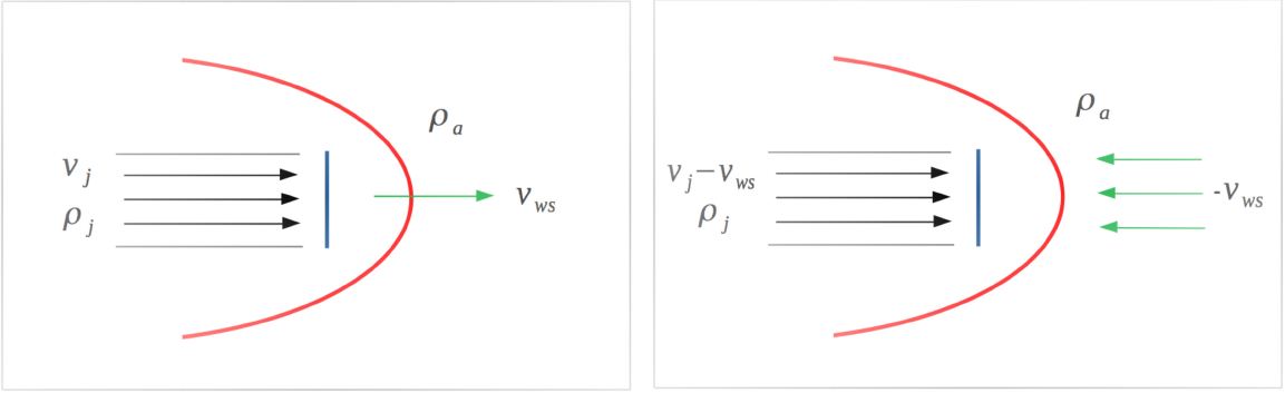
Fig. 1 Jet head working surface in a reference frame at rest with respect to the outflow source (left) and in a reference frame moving along with the working surface (right). The bow shock is shown in red and the jet shock in blue. The color figure can be viewed online.
The right panel of Figure 1 shows the situation seen in a reference frame at motion with the jet head. For a hypersonic flow, the two working surface shocks are strong, so that the post-shock gas pressures are given by:
for the bow shock, and
for the jet shock (assuming that the jet and the environment have the same specific heat ratio γ). In this equation, v j and ρ j are the velocity (with respect to the outflow source) and the density of the material that is presently entering the jet shock.
If the working surface is moving with a constant velocity the condition
is satisfied. This is called the ram-pressure balance condition. This condition is also valid for a working surface moving with a variable velocity as long as the inertia of the material between the bow shock and the jet shock is negligible, which is the case if most of the material is ejected sideways from the working surface into a jet cocoon.
From equation (29) we find that
Clearly, the shock velocity associated with the bow shock is v bs = v ws and the shock velocity of the jet shock is:
We now consider the equation of motion v ws = dx ws /dt for the working surface. Setting v j = u 0(τ) (i.e., the velocity of the material entering the working surface is equal to the ejection velocity at the corresponding ejection time τ), we then have:
The ejection time τ of the material entering the working surface is obtained from the free-streaming relation
where t is the evolutionary time (see equation 4). Solving for t and differentiating with respect to τ we obtain
Combining equations (32) and (33), we obtain:
The density of the jet material entering the working surface is ρ j = ρ(x ws ,t) (see equation 5), which for our chosen ejection velocity variability (see equation 1) becomes:
Finally, from equations (34) and (35) we obtain:
In order to proceed it is now necessary to specify the form of ρ 0(τ). We therefore consider the two cases of constant mass loss rate and constant ejection density.
For
It is convenient to use the dimensionless variables:
In terms of these variables, equation (37) is
In Appendix A, it is shown that an approximate analytic solution of equation (39) can be constructed as a non-linear average of a “near” and a “far field” analytic solution (see equations 51 and 52), which in terms of the respective dimensional variables is
Setting ρ 0 = const. in (36) and taking the square of the equation, we obtain:
Proposing a power law solution, we find that
We therefore find a quadratic dependency on the ejection time.
Using equations (11) and (42) we then obtain:
where β 0 is given by equation (24). This implies a quadratic dependence on the evolutionary time.
In the
and the β0≫1 limit leads to
3. THE NUMERICAL SIMULATIONS
In order to check our analytical solutions we computed a set of 2D axisymmetric simulations for both the constant mass loss rate and constant ejection density cases. For the simulations we use a code that solves the ideal gas-dynamic (Euler) equations in a fixed two dimensional grid. The code uses a second order Godunov type method with the HLLC (Toro et. al. 1994) approximate Riemann solver, including a linear reconstruction of the primitive variables with the minmod slope limiter to avoid spurious oscillations. In order to use cylindrical coordinates, the appropriate geometrical source (∝ 1/r) terms are included after each time step in an operator splitting fashion. Additionally, we incorporated the cooling function dependent on density, metallicity and temperature in the energy equation (also as source term) as proposed by Wang et al. (2014), which we compute assuming a solar metallicity.
In order to stabilize the method an artificial diffusion with a (dimensionless) value of 0.01 was added to all of the equations, and a Courant number of 0.2 was used. The code is written in fortran90 and is parallelized with the Message Passing Interface. We used a computational grid with a size of 0.05 and 0.2pc along the r and x directions, respectively. The spatial resolution was ≈ 6.89au, corresponding to 600 × 6000 cells along the radial and axial directions.
3.1. Initial and Boundary Conditions
We model jets propagating into a uniform, quiescent environment, and consider the values n a = 100 cm−3 and n a = 5000 cm−3 for the environmental density. For convenience, from now on we will use number density instead of mass density. We consider a mean molecular weight of µ = 1.3. We also consider the cases of jets with a constant mass loss rate and a constant ejection density.
In all simulations, we consider the ejection velocity variability given by equation (1) with a = 100 kms−1 per millenium = 3.17 × 10⁻⁴ cms−2. An initial jet radius r j = 300AU (the cross section being σ = πr j 2) and a temperature T = 100K (for both the jet and the environment) were imposed in all models.
We therefore compute four models, two with constant ejection density (which we
label n
100 and n
5000, with the subscript giving the ambient density in
cm−3) and two with constant mass loss rate (which we label
In the constant mass flux cases, we find a maximum jet density of n j = 1.56×107 cm−3, and a minimum jet density of n j = 6.24×103 cm−3, corresponding to an ejection time τ = 1yr, and τ = 2500yr, respectively.
We should note that the parameters we have chosen are inspired in the characteristics of “classical” HH jets such as HH 34 and HH 111, which have:
radii ≈ 100 AU (Reipurth et al. 2002) and ≈ 300 AU (Reipurth et al. 1997), for HH 34 and HH 111, respectively. We chose the larger of these two radii in order to have a better resolution of the jet in our numerical simulations. These jet radii are measured in the “jet knot chain” at distances of ≈ 10'' (corresponding to ≈ 6 × 1016 cm) from the outflow sources, and not in the considerably broader HH 34S and HH 111V “heads”;
full spatial velocities (i.e., combining radial velocities and proper motions) between 200 and 300 km s−1 (Hartigan et al. 2001; Reipurth et al. 2002) and lengths (out to HH 34S and HH 111V) of ≈ 8 × 1017 cm. We have then made a choice of a = 100kms−1 per millenium (see above), which after an evolutionary time of ≈ 2500 yr produces a jet head with a position and velocity similar to the ones of HH 34S and HH 111V (see the following section). The simulations are stopped at this time (i.e., at 2500 yr);
mass loss rates in the 10
even though the ambient densities in HH 34 and HH 111 are of ≈ 10 cm−3 (19), we have chosen higher environmental densities (of 100 and 5000 cm−3, see above) in order to have a substantial braking effect and to obtain larger differences between the center of mass and rampressure balance solutions.
4. RESULTS
We computed four numerical simulations, two with a constant ejection density (models
n
100 and n
5000) and two with a constant mass loss rate (models
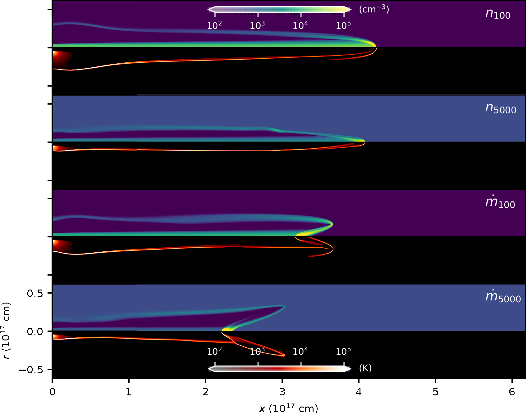
Fig. 2 Numerical density and temperature stratifications obtained from our four models (see the text and Table 1), at an evolutionary time of 2500 years. For each model, we show the number density (top half) and temperature (bottom half) in logarithmic color scales. The axial and radial axes are given in units of 1017 cm. In the constant mass loss rate models the jet density and the pressure drop quite considerably, leading to the formation of internal “crossing shocks”. The color figure can be viewed online.
Generally, the highest densities and temperatures are found in the on-axis regions of
the jet heads. The jet heads of the models with constant ejection density (models
n
100 and n
5000) have traveled to distances from the outflow source larger than the
ones of constant mass loss rate (
As a result of the lower jet beam density and pressure, the constant mass loss rate models develop an incident/reflected crossing shock structure, which (in the incident shock region) leads to the production of faster off-axis motions in the jet head (see the two bottom panels of Figure 2). This kind of structure is always found in jet simulations with appropriate parameters, i.e. simulations where the jet is under-dense and under-pressured with respect to the environment during its evolution (see, e.g., Raga 1988; Downes & Ray 1999).
The upper left panel of Figure 3 shows the
position of the bow shock (dash-dotted blue line) and jet shock (dotted blue line)
as a function of time for the
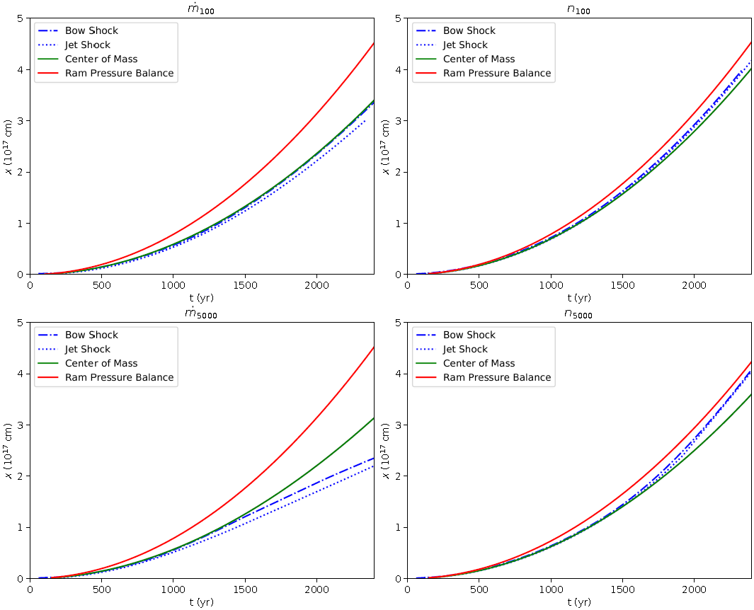
Fig. 3 Position of the jet head as a function of time for the constant mass loss rate models (left panels) and the constant ejection density models (right panels). The red solid line shows the ram-pressure balance solution and the green dashed line shows the center of mass solution. The dash-dotted line shows the bow shock and the dotted line the jet shock positions obtained from the numerical simulations. The color figure can be viewed online.
The upper right panel of Figure 3 shows the timedependent position of the jet head for the n 100 constant ejection density model. For times < 1500 yr, the jet and bow shock positions (obtained from the numerical simulation) quite closely follow the center of mass analytic solution. At larger times, the jet and bow shock positions lie above the center of mass solution, and begin to approach the ram-pressure balance solution. At all times, the positions of the jet and bow shock lie in between the working surface positions predicted by the two analytic models.
The lower left panel of Figure 3 shows the
evolution of the jet head for the
The strong departures from the simple, cylindrical structure assumed in the analytic models occurs because at increasing times the jet density (and pressure) drop quite considerably in this model, leading to the formation of internal “crossing shocks”. These shocks then lead to the formation of complex off-axis structures in the jet head (see the two bottom panels of Figure 2).
The lower right panel of Figure 3 shows the dynamics of the jet head for the n 5000 constant ejection density model. This model shows jet and bow shock positions that initially follow the center of mass analytic model, and at times t > 1500 yr tend to approximate the ram-pressure balance model.
Finally, we calculate the relative position differences ∆x a /x cm = x/x cm − 1, with x cm being the position of the “center of mass jet head” (see equations 17 and 21). The distance from the source x a corresponds either to the bow shock or jet shock positions (obtained from the numerical simulations), or to the position of the “ram-pressure balance jet head” (see equations 40 and 43). Figure 4 shows the relative position differences (with respect to the center of mass position for the jet head) for all of our computed models. The first thing to note (see the red lines in the two right panels of Figure 4) is that the relative position difference between the center of mass and ram pressure balance solutions does not strongly depend on time for the constant ejection density models (a result that can be seen by comparing equations 21 and 42). This result does not strictly hold for the constant mass loss rate models (red lines in the left panels of Figure 4).
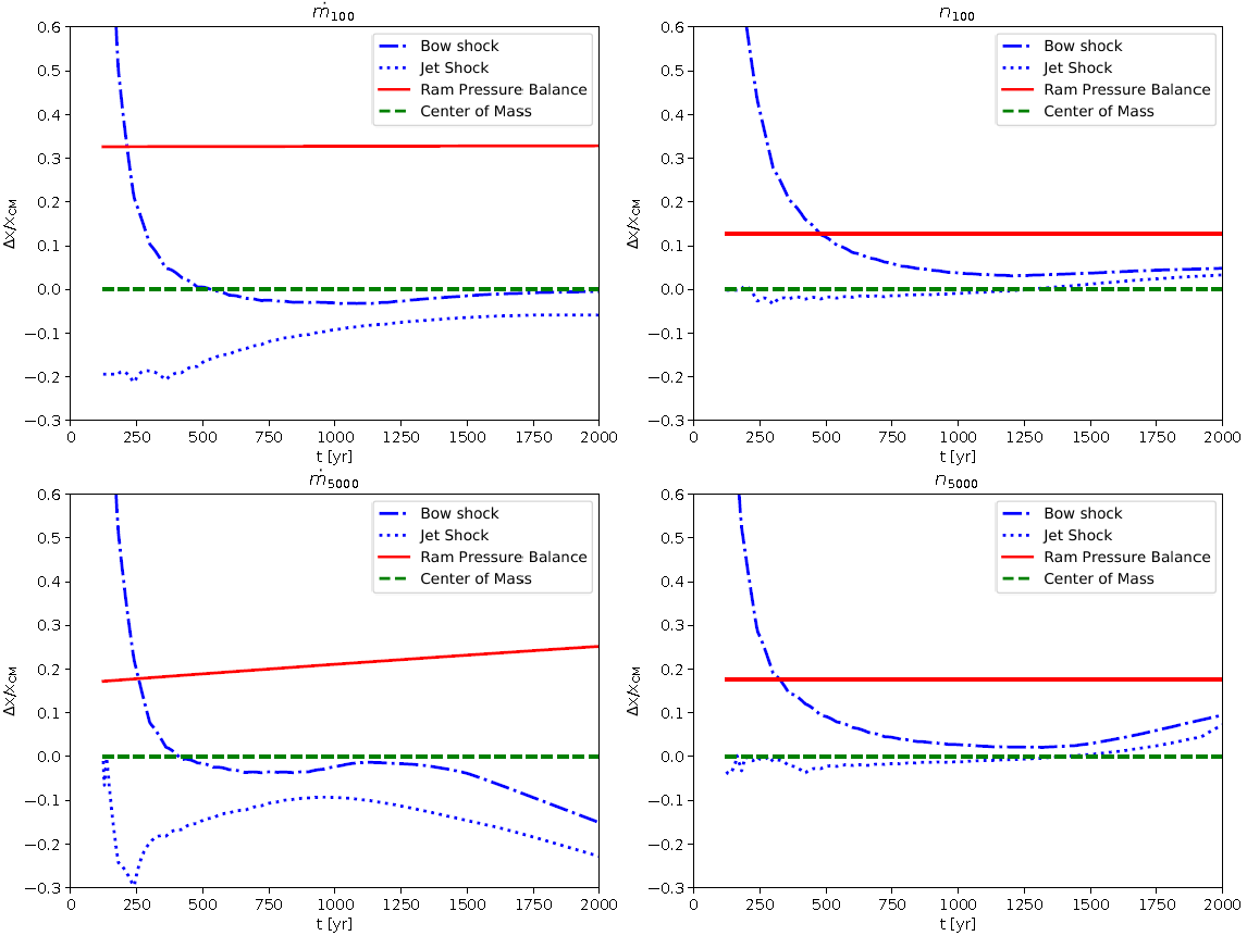
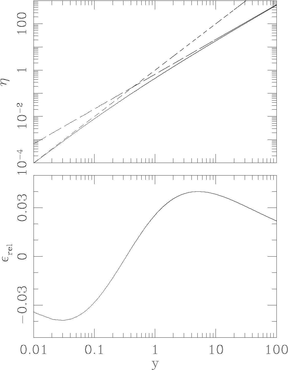
Fig. 4 The relative differences of the ram-pressure balance solution (solid red line), the numerical bow shock (dashdotted blue line) and jet shock positions (dotted blue line) with respect to the center of mass working surface solution (the dashed, green line showing the ∆x/x cm = 0 line) as a function of time t. The results obtained for our four models (see Table 1) are shown (constant mass loss rate models on the left, and constant ejection density models on the right). The color figure can be viewed online.
For the constant mass loss rate models we see that for t > 550 yr the bow and jet shock positions remain below the center of mass working surface position, with negative ∆x values (see the left panels of Figure 4). For the constant ejection density models (right panels of Figure 4) we see an initial convergence to the center of mass solution of the bow and jet shock positions, and for t > 1300 yr we see progressively larger, positive values for ∆x/x cm (starting to approach the ram-pressure balance working surface position).
5. DISCUSSION
We have presented a first attempt to compare the analytic ram-pressure balance (Raga & Kofman 1992) and center of mass (Cantó et al. 2000) formalisms (for obtaining the motions of working surfaces in variable ejection jets) with axisymmetric numerical simulations. To this effect, we chose the relatively simple problem of the leading head of a jet produced with an ejection velocity that increases linearly with time. We explored the cases of a time-independent mass loss rate (in which the ejection density scales as the inverse of the ejection velocity) and of a constant ejection density. From the simulations we computed the on-axis positions of the jet shock and bow shock, and compared them with the predictions of the analytic models (in which the jet and bow shock are assumed to be spatially coincident).
For three of our four simulations (models n
100, n
5000 and
It is clear that right after a working surface is formed, the two associated shocks
are very close to each other (with a separation
It is possible to obtain analytic estimates of the separation between the two shocks (and therefore the mass of the gas within the working surface) with different degrees of complexity (and accuracy), following the approaches developed for determining the shock standoff distance in blunt body flows (see, e.g., the book of Hayes & Probstein 2003 and Cantó & Raga 1998). Here, we present a very simple estimate of the mass within a working surface.
In the stationary state (i.e., after the initial regime of growing separation between the two working surface shocks), the mass M ws within the two working surface shocks is:
where
Also, the total mass that has been fed into the working surface is
where t d = x ws /v ws is the dynamical timescale (with x ws being the position and v ws the velocity of the working surface).
Combining equations (46-48) we obtain
In this equation, we have considered that the M ws /M in ≤ 1 condition has to be satisfied (with M ws = M in for the initial, mass conserving regime, and M ws < M in when the sideways ejection from the working surface becomes important), while our analytic estimate can give values > 1 because of its implicit assumption of a balance between the mass rates into and out of the working surface (which is not satisfied in the early evolution of the working surface, as discussed above). Clearly, for the case of an accelerating working surface (as the one that we obtain from our variable ejection models), the derivation of equation (49) should be done evaluating the appropriate integrals (see § 4 of the paper of Lim et al. 2002), but the simple derivation shown above still gives the correct scaling properties.
We now consider that the transition between the mass conserving and efficient mass losing working surface regimes (which can be described with the “center of mass” and “ram-pressure balance” equations of motion, respectively) occurs when M ws /M in ≈ 1/2 (i.e., that the working surface has lost half of the processed jet material). Therefore, the position x t of the working surface at which the transition between the center of mass and ram pressure balance regimes occurs can be estimated setting M ws /M in = 1/2 in equation (49), which gives:
Setting c 0 = 3 km s−1 (see above), r j = 300 au (see § 3) and a velocity v ws ≈ 200 km s−1, we then obtain x t ≈ 3 × 1017 cm, This is the correct order of magnitude for the location of the transition between the “mass conserving” center of mass and the “efficient mass losing” ram-pressure balance regimes for the working surface found in our n 100 and n 5000 numerical simulations (see Figure 3).
To summarize, we find that numerical simulations of a jet with a linearly accelerating ejection velocity vs. time produce a leading head which at early times can be analytically modeled with the center of mass formalism, and (for appropriate flow parameters) at later evolutionary times approaches the ram-pressure balance solutions. The distance from the source at which the transition between these two regimes occurs can be estimated with equation (50). This result holds provided that during its time-evolution the jet does not become under dense/under pressured, in which case strong departures from the analytic solutions are found.
6. CONCLUSIONS
This paper presents a first attempt to compare analytic solutions based on both the “ram-pressure balance” and “center of mass” formalisms with hydrodynamical (axisymmetric) simulations. For this comparison we have studied the case of a linearly increasing ejection velocity as a function of time (and two different forms for the ejection density, see § 2).
This simple ejection variability could apply to the early evolution of an HH outflow, and is relevant for the problem of entrainment of environmental molecular material into the jet head (see Lim et al. 2002) and the potential destruction of molecules by shocks, particularly in the jet head. Since a direct application to the observed, evolved, HH jets is not straightforward, the interest of our work is primarily theoretical.
While full analytic solutions for different forms of the ejection variability have been found in the past with the “center of mass” formalism (see Cantó et al, 2000 and Cantó & Raga 2003), no solutions (except the trivial one for the constant ejection case) have been found with the “ram-pressure balance” equation of motion for the working surfaces. We were surprised to find that the “linearly accelerating” ejection velocity case does lead to a full, analytic rampressure balance solution for the case of a constant ejection density (though we managed to find only an approximate analytic solution for the constant mass loss rate case). This result implies that ram-pressure balance analytic solutions might also exist for other ejection velocity/density variability combinations.
Comparing the center of mass and the rampressure balance solutions with axisymmetric numerical simulations (with the same parameters) we find that for the case of over-dense jets (with higher densities in the jet side of the leading working surface) the numerical results initially follow the center of mass solution, and at later times approach the ram-pressure balance analytic solution. This result shows a satisfying consistency between the analytic approaches and the numerical solutions with the full (axisymmetric) hydrodynamic equations. Not unexpectedly, we do not find a good agreement between the analytic and numerical results for cases in which the jet density drops to values lower than the environmental density, as the jet beam then develops internal shocks (in the numerical solutions) that affect the motion of the leading working surface.
Clearly, it would be interesting to extend this comparison between numerical simulations and analytic solutions of variable jets to the case of jets with “internal working surfaces” within their beams. This problem, which would clearly have much more direct applications to observed HH jets, is left for a future study.