


 nueva página del texto (beta)
 Inglés (pdf)
 Artículo en XML
 Referencias del artículo
 Enviar artículo por email
 Citado por SciELO
  Similares en
SciELO
Similares en
SciELO 
 Permalink
1. Introduction
In different stellar outflows, one sometimes finds clump-like flows with an emitting “trail” (linking the clumps to the outflow source) with a “Hubble law” of linearly increasing velocities with distance from the source. This kind of structure is observed in some outflows from young stars (most notably in the Orion BN-KL outflow, see e.g. Allen1983, Bally2017 and Zapata 2011 and in some planetary (PN) and protoplanetary (PPN) nebulae (see, e.g., Alcolea 2001 and Dennis 2008). A second, striking outflow with multiple “Hubble tail clumps” has been recently found by Zapata 2020.
Following the suggestion of Alcolea 2001 that the observed “Hubble law tail” clumps were the result of “velocity sorting” of a sudden ejection with a range of outflow velocities, Raga 2020a,Raga 2020b developed a model of a “plasmon” resulting from a “single pulse” ejection velocity variability. In this model, an ejection velocity pulse of parabolic Raga 2020a or Gaussian Raga 2020b time-dependence forms a working surface (the “head” of the plasmon) followed by the material in the low velocity, final wing of the ejection pulse (forming the Hubble law “tail”). These authors called this flow the “head/tail plasmon”, adapting the name proposed by De Young 1967 for a clump-like outflow.
In the present paper, we study an alternative type of “single pulse outflow” that also produces a structure with a Hubble law of linearly increasing velocities with increasing distances from the outflow source, We propose a cylindrical ejection with:
a “square pulse” time-dependent ejection velocity, with a sudden “turning on” at an ejection time τ = 0 and a “turning off” at τ = τ 0,
a parabolic initial cross section for the ejection velocity (with a peak, on-axis velocity and 0 velocity at the outer edge r j ).
This is in contrast to the single pulse outflows studied by Raga 2020a, Raga 2020b, who proposed parabolic or Gaussian time-dependencies for the velocity and a top-hat cross section ejection for the ejection.
The paper is organized as follows. In § 2, we describe an analytic model, based on the “center of mass” formalism of Canto 2000, which leads to a simple solution for the motion of the working surface produced by the (non-top hat cross section) ejection pulse. In § 3, we present an axisymmetric numerical simulation (with parameters appropriate for a high velocity knot in a PN), and compare the obtained results with the analytic models. Predictions of position-velocity (PV) diagrams are done from the numerical model. Finally, the results are discussed in § 4.
2. The Analytic Model
2.1. The Shape of the Working Surface
Let us consider a hypersonic, cylindrical ejection with a time-dependent, “square pulse” ejection velocity, and a non-top hat cross section. The ejected material will be free-streaming (because the pressure force is negligible) until it reaches a leading working surface (or “head”) formed in the interaction between the outflow and the surrounding environment. This situation is shown schematically in Figure 1.
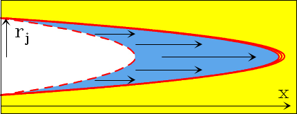
Fig. 1 Schematic diagram showing the interaction of an ejection pulse (of duration τ 0 and initial radius r j , travelling along the x-direction) with a non-top hat ejection velocity cross section interacting with a uniform environment. The outflow interacts with the environment forming a two-shock, curved working surface (thick, solid red curve). At evolutionary times t > τ 0 the source is no longer ejecting material, and therefore an empty region (limited by the dashed, red curve) is formed close to the outflow source. At large enough times, all of the ejected material will join the working surface, and the empty region will be bounded by the bow shock. The color figure can be viewed online.
If the material in the working surface is locally well mixed, the center of mass formalism of Canto 2000 will give the correct position x cm of the working surface for all radii r in the cross section of the outflow. Then,
where ρ a (x) is the (possibly position-dependent) ambient density, τ ' is the time at which the flow parcels were ejected. u 0(r,τ ') and ρ 0(r,τ ') are the time-dependent velocity and density ejection cross sections (respectively),
is the position that the fluid parcels would have if they were still in the free-flow regime and τ is the time at which the parcels now (i.e., at time t) entering the working surface were ejected. This time τ can be found by appropriately inverting the free-streaming flow relation:
Now, let us assume that we have an ejection pulse with a velocity
with constant v 0. For τ < 0 and τ > τ 0 there is no ejection. The function f(r) is the radial profile of the ejection velocity, which we will assume has a peak at r = 0 and low velocities at the outer radius r j of the cylindrical ejection. We will furthermore assume that the ejection density ρ 0 is time independent, and that the outflow moves into a uniform environment of density ρ a .
We now introduce the ejection velocity given by equation (4) and constant ρ 0 and ρ a (see above) in equations (1-2) to obtain:
Where
is the environment-to-outflow density ratio. This equation can be inverted to obtain x cm as a function of t and τ:
where τ is the ejection time of the material entering the working surface at an evolutionary time t (see equation 3).
Now, as t grows, the ejection time τ also grows. and eventually reaches τ 0. For τ > τ 0, all of the ejected material (at a given radius r) has fully entered the working surface, and for larger times the position of the working surface evolves following equation (7) with τ = τ 0.
It is also possible to obtain x cm fully as a function of evolutionary time t by combining equations (3) and (4) to obtain
valid for
which (not surprisingly) corresponds to the constant velocity motion predicted from a simple “ramppressure balance” argument. This solution was derived for the head of a constant velocity, non-top hat cross section jet by Raga et al. (1998).
For τ > τ 0, the position is given by equation (7) with τ = τ 0:
The transition between the regimes of equation (9) and (10) occurs at the evolutionary time t c when the material ejected at τ 0 catches up with the working surface. The position of the last ejected material is:
and it catches up with the working surface when t = t c and x 0 = x ws . We can now use the value of x ws obtained from equations (9) or (10), which when substituted in equation (11) both lead to:
which is independent of r. Therefore, at a time t c , the material of the pulse ejected at all radii is fully incorporated into the working surface. At a time t c , the working surface has a shape:
obtained by combining equations (9) and (12).
2.2. The Velocity Structure
The velocity of the material within a fully mixed working surface is directed along the x-axis (see Figure 1). The position-dependent velocity can be straightforwardly obtained by calculating the timederivative of the x cm (r,t) locus of the working surface (given by equations 9 and 10, depending on the value of t).
For t ≤ t c (see equation 12), from equation (9) we obtain:
Therefore, the velocity in the curved working surface has a “Hubble law” of linearly increasing velocities as a function of distance along the x-axis, with a slope of 1/t.
For t > t c (see equation 12), from equation (10) we obtain:
Again, the velocity as a function of distance follows a linear, “Hubble law”. The
slope of this law (see equation 15) is 1/t for
t = t
c
, and approaches a value of
2.3. Solutions for Different σ Values
If we choose values for the density ratio σ = ρ a /ρ 0, from equations (9-10) we obtain the position x ws and from equations (14-15) the velocity of the working surface on the symmetry axis. The positions and velocities obtained for σ = 0, 0.1, 0,5, 1.0 and 2.0 are shown in Figure 2.
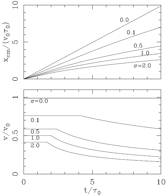
Fig. 2 Position (top) and axial velocity (bottom) of the head of the plasmon as a function of time. The curves are labelled with the values of σ used to calculate the solutions (see equations 9, 10, 14 and 15).
For σ = 0 (the “free plasmon”) the plasmon head moves at a constant velocity v 0 (see equation 4). For σ > 0, the working surface moves at a constant velocity (given by equation 14) for t ≤ t c (see equation 12), and has a monotonically decreasing velocity for t > t c . The velocity at all times has lower values for larger σ.
In order to illustrate the shapes that the plasmon (i.e., the working surface) can take, we choose a parabolic ejection velocity cross section (see equation 4):
where r j is the radius of the cylindrical outflow.
In Figure 3, we show the time-evolution of the flow for three different values of the environment-toejection density ratio: σ = 0, 0.1 and 0.5. For σ = 0, the time at which the ejected material fully enters the working surface is t c → ∞ (see equation 12). For σ = 0.1 and 0.5, we obtain t c = 4.1τ 0 and 2.41τ 0, respectively. The shapes shown in Figure 3 were obtained using equation (9) for times t ≤ t c and equation (10) for t > t c (this case applies only to the t = 3 and 4τ 0 frames of the σ = 0.5 case).
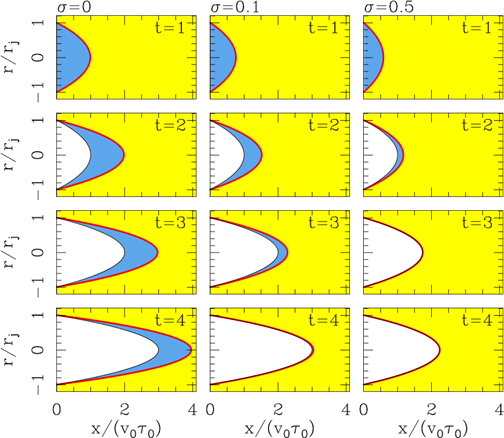
Fig. 3 Solutions for an outflow pulse with a parabolic ejection velocity cross section (see § 2.3). The three columns show the time-evolutions obtained for different values of σ = ρ a /ρ 0, and are labelled with the corresponding σ (above the top graphs). The four lines correspond to different evolutionary times: t = τ 0 (top), 2τ 0, 3τ 0 and 4τ 0 (bottom). The working surface is shown with the thick, solid line, and the “empty cavity” region is shaded white. The blue region (not always present) is the ejected material which has still not been incorporated into the working surface. The color figure can be viewed online.
Also shown in Figure 3 is the “empty region” formed for t > τ 0 (i.e., when the ejection has already stopped) close to the outflow source (see equation 11). In the σ = 0 case, the working surface moves freely, and therefore the ejected material (shown in blue in Figure 3) never catches up with it. In the σ = 0.1 case, in the t = 4τ 0 frame most of the ejected material has already caught up with the working surface, and in the σ = 0.5 case in the t = 3 and 4τ 0 frames (which have t > t c , see above) all of the outflow material is within the working surface, and the “empty region” fills the volume between the outflow source and the working surface.
3. A NUMERICAL SIMULATION
3.1. Flow Parameters
In order to illustrate in more detail the full characteristics of the flow, we compute an axisymmetric numerical simulation of the “parabolic cross section plasmon” described in § 2.3 using the walicxe-2D code (Esquivel et al. 2009). We choose parameters appropriate for a high velocity clump in a PN: an axial velocity with an on-axis value v 0 = 200 km s−1 (decreasing parabolically to zero at a radius r j , see equation 16), an initial radius r j = 1016 cm, an ejection atom+ion number density n 0 = 104 cm−3 (independent of radius) and an ambient density n a = 100 cm−3. Initially, both the outflow and the environment have a 104 K temperature. The ejection is imposed at t = 0 (at the beginning of the simulation) and ends at a time τ 0 = 100 yr. For these parameters, the environment to outflow density ratio has a value σ = 0.1, and we then expect the ejected material to be fully incorporated into the working surface at a time t c = 416.2 yr (see equation 12).
We assume that all of the flow is photoionized by the central star of the PN. We consider this photoionization in an approximate way by imposing a minimum temperature T = 104 K and full ionization for Hydrogen throughout the flow. The parametrized cooling function of Biro & Raga (1994) is used for T > 104 K.
The computational domain has a size of (35, 8.75) × 1016 cm (along and across the outflow axis, respectively), resolved with a 7-level binary adaptive grid with a maximum resolution of 8.54 × 1013 cm. An inflow boundary is applied at x = 0 and r > r j for t < τ 0, a reflection boundary is applied outside the injection region (at x = 0) and on the symmetry axis, and a free outflow is imposed in the remaining grid boundaries.
3.2 Results
We have run the simulation described in § 3.1 for a total time of 600 yr. Figures 4 and 5 show timeframes (at times t = 100, 200, 300, 400, 500 and 600 yr) of the resulting density stratification. In these figures, we show the shape of the working surface (equations 9 and 10). For times t ≤ t c = 416.2 yr (see § 3.1), we also show the inner edge of the “empty cavity” of the analytic model (equation 11). For t > t c , all of the region inside the working surface is in the “empty cavity” regime, and for t ≤ τ 0 = 100 yr there is no empty region.
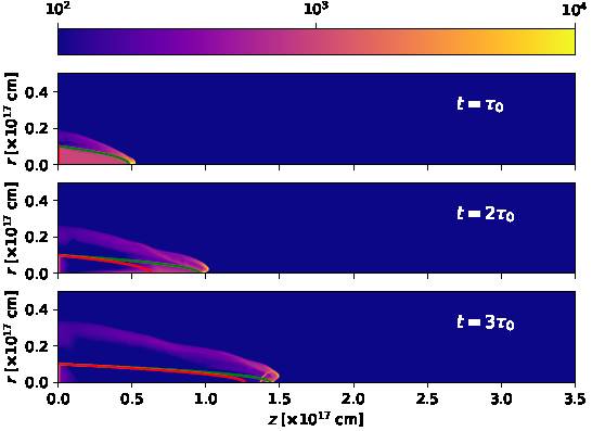
Fig. 4 Number density stratifications obtained from the numerical simulation for times t = 100, 200 and 300 yr. The densities are shown with the logarithmic colour scale given by the top bar (in cm−3). The shape of the working surface obtained from the analytic model is shown with the green curve, and the inner limit of the analytic “empty cavity” is shown with the red curve. The distances along and across the outflow axis are given in units of 1017 cm. The color figure can be viewed online.
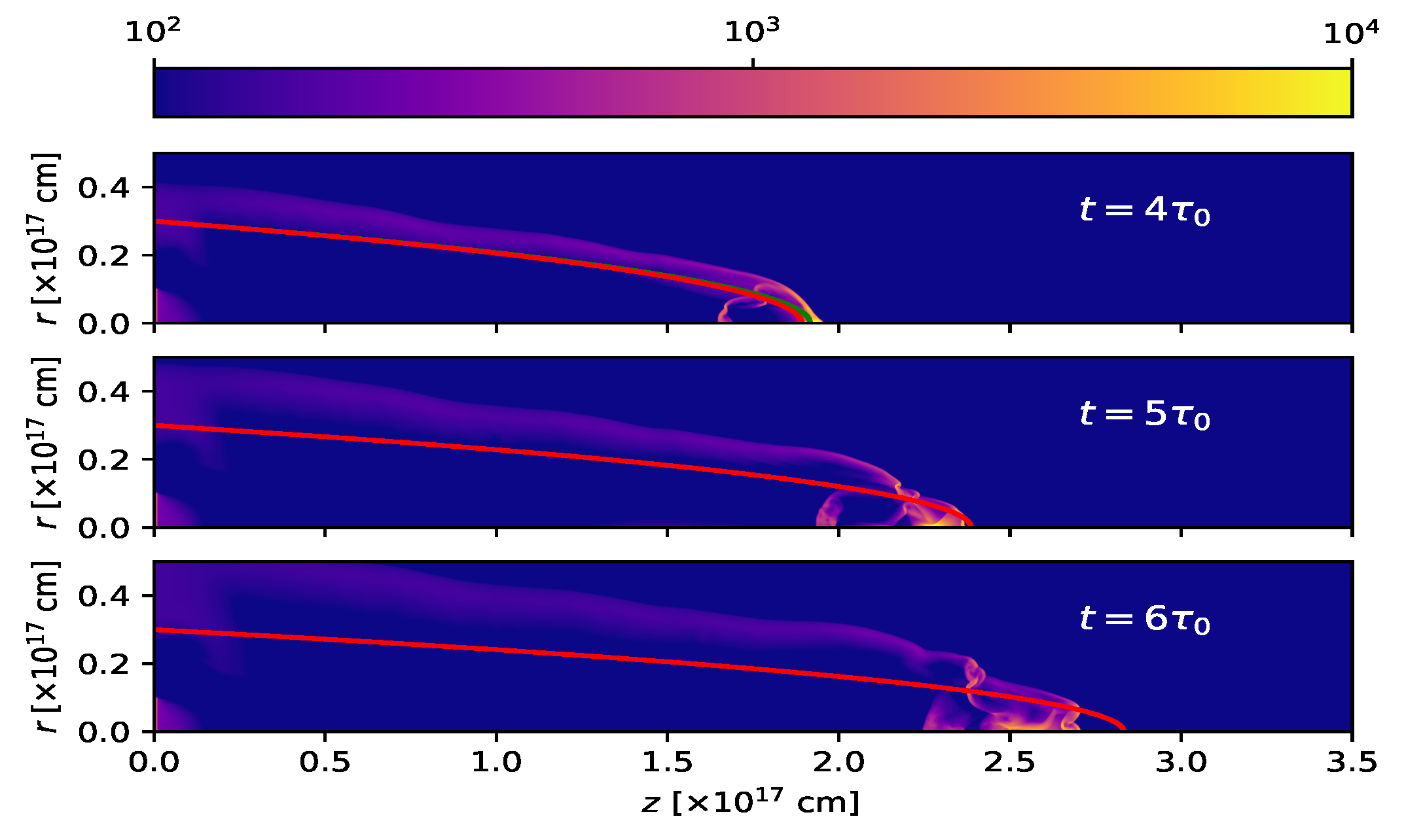
Fig. 5 The same as Figure 4, but for times t = 400, 500 and 600 yr. The color figure can be viewed online.
It is clear that even though at early times (see the t = τ 0 frame of Figure 4) the working surface of the numerical simulation has a shape that partially agrees with the analytic model, at later times the working surface has bow shock wings which are considerably broader than the analytic prediction (see the remaining frames of Figures 4 and 5). This difference is partly due to the lack of perfect mixing (assumed in the analytic model) between outflow and environment material in the numerical simulation. The other effect that pushes out material sideways from the head of the working surface is the radial gas pressure gradient (also not included in the analytic model). However, the position of leading region of the working surface approximately agrees with the analytic model at all times (see Figures 4 and 5).
We have computed the recombination cascade Hα emission coefficient, and integrated it through lines of sight in order to compute intensity maps. Figures 6 and 7 show the emission maps computed assuming a 30◦ angle between the outflow axis and the plane of the sky, for times t = 100, 200, 300, 400, 500 and 600 yr.
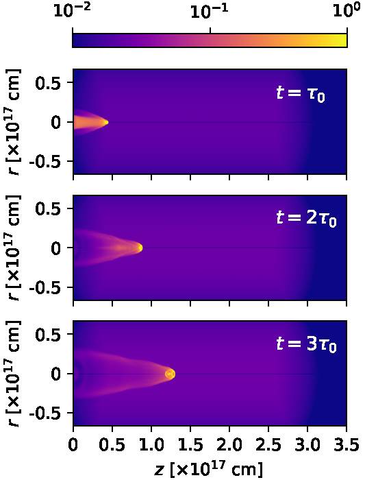
Fig. 6 Hα maps obtained from the numerical simulation for times = 100, 200 and 300 yr. The maps are computed assuming a 30 angle between the outflow axis and the plane of the sky. The emission (normalized to the peak emission of each map) is shown with the logarithmic colour scale given by the top bar. The distances along and across the outflow axis are given in units of 1017 cm. The color figure can be viewed online.
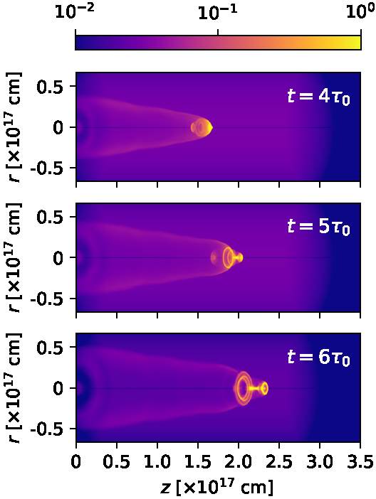
Fig. 7 The same as Figure 6, but for times t = 400, 500 and 600 yr. The color figure can be viewed online.
From Figures 6 and 7, we see that the earlier maps (the t = 100 and 200 yr, top two frames of Figure 6) show the emission from the ejected material before it reaches the working surface. In all of the later maps, we see a bright, compact component in the leading, on-axis region of the working surface, and the emission of extended bow shock wings trailing this clump.
With the Hα emission coefficient we have also computed predicted position-velocity (PV) diagrams. These PV diagrams correspond to long-slit spectra obtained with a “narrow” spectrograph slit with a full projected width of 2 × 1016 cm straddling the outflow axis (see Figures 8 and 9) and with a “wide” spectrograph slit that includes all of the emission of the bow shock (see Figures 10 and 11), and show the emission as a function of position along the outflow axis and radial velocity (along the line of sight). Figures (8, 9) and (10, 11) show the PV diagrams computed for a 30◦ orientation of the outflow axis with respect to the plane of the sky, and for times t = 100, 200, 300, 400, 500 and 600 yr.
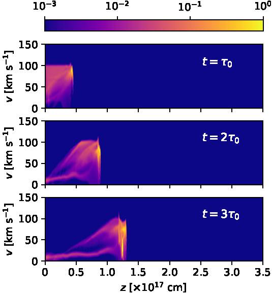
Fig. 8 Hα position-velocity diagrams obtained from the numerical simulation for times t = 100, 200 and 300 yr. These PV diagrams have been calculated assuming that a long spectrograph slit with a projected full width of 2 × 1016 cm straddles the symmetry axis of the flow. The maps are computed assuming a 30◦ angle between the outflow axis and the plane of the sky. The emission (normalized to the peak emission of each map) is shown with the logarithmic colour scale given by the top bar. The distances along the outflow axis are given in units of 1017 cm, and the radial velocities in km s−1. The color figure can be viewed online.
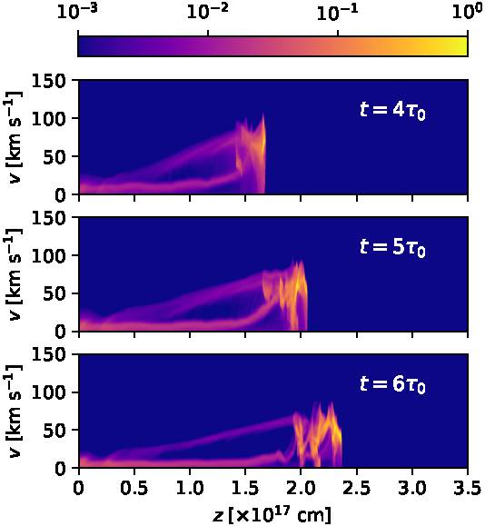
Fig. 9 The same as Figure 8, but for times t = 400, 500 and 600 yr. The color figure can be viewed online.
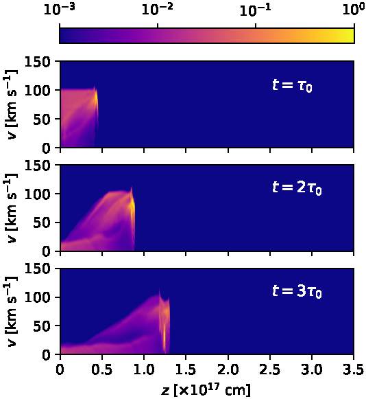
Fig. 10 The same as Figure 8, but with PV diagrams calculated for a wide spectrograph slit that straddles the symmetry axis and includes all of the emitting region of the flow. The color figure can be viewed online.
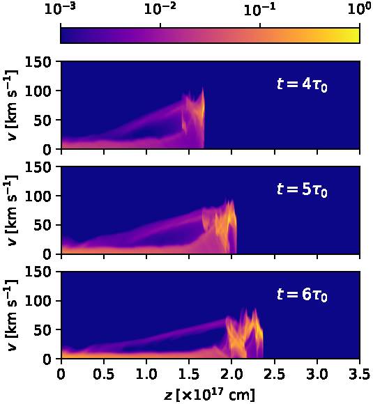
Fig. 11 The same as Figure 9, but with PV diagrams obtained with a wide spectrograph slit that includes all of the emitting region of the flow. The color figure can be viewed online.
From these figures it is clear that in all of the PV diagrams we see:
qualitatively very similar results for slits of different widths (seen comparing Figure 8 to Figure 10, and 9 to 11),
a bright, compact emission feature at the position and velocity of the on-axis, leading region of the working surface,
an approximately linear ramp of increasing radial velocities, ending at the position of the leading clump.
Apart from these two components, in the earlier frames (t = 100 and 200 yr, the two top frames of Figure 8) we see the ejected material (at a projected velocity of 100 km s−1) before it reaches the working surface. This component disappears at later times, since all of the ejected material has then been incorporated into the working surface. Also, at all times we see a low velocity component, which corresponds to environmental material that has been shocked by the far bow shock wings and has not mixed with the rest of the flow.
4. SUMMARY
We have studied the flow resulting from a constant density, collimated, cylindrical non-top hat cross section ejection of material over a finite time τ 0. We first calculate an analytic model (based on the “center of mass formalism” of Cantó et al. 2000) with which we obtain analytic expressions for the time-evolution of the working surface produced by the interaction of the ejection with a uniform environment.
This solution has two regimes:
a working surface which is being fed by the ejected material (see equation 9). This solution was previously derived by Raga et al. (1998),
a working surface in which all of the ejected material has already been incorporated (see equation 10).
The transition between the two regimes occurs at the time t c given by equation (12). For t < t c , the region inside the working surface is partly filled by the ejected material (with an inner cavity with a boundary given by equation 11). For t > t c , the region within the working surface is “empty” (i.e., as in the ballistic analytic model, see Figure 3).
For t < t c , the working surface moves at a constant velocity, and for t > t c it slows down, more strongly for larger values of the environment-toejection density ratio σ = ρ a /ρ 0 (see Figure 2). For these two regimes, we find that the material in the working surface has a linear velocity vs. x (the position along the outflow axis) dependence, given by equations (14) and (15).
We also compute an axisymmetric numerical simulation, with conditions appropriate for a high velocity clump in a PN. We find that the density structure
initially shows a working surface and a low density cavity that agree well with the analytic predictions (see Figure 4). However, at later times the numerical working surface develops bow shock wings that are considerably broader than the ones of the analytic prediction (see Figures 4 and 5). The position of the leading region of the working surface shows a reasonably good agreement with the analytic model for all of the computed times.
From the numerical simulation, we have calculated Hα maps (Figures 6 and 7) and PV diagrams (Figures 8 to 11). We find that the PV diagrams do show the linear radial velocity vs. position “Hubble law” predicted from the analytic models (see Figures 8 and 9).
Therefore, we have found a new way of straightforwardly obtaining clump-like outflows with a “Hubble law” linear radial velocity ramp joining them to the outflow source. This is an alternative scenario to the one of the “single peak radial velocity pulse” model of Raga et al. (2020a,b), which also produces “Hubble law clumps”. Clearly, these two possibilities are useful as guidelines to obtaining detailed models of structures with these characteristics in PN (see, e.g., Dennis et al. 2008) or in outflows in star formation regions (see, e.g., Zapata et al. 2020).
We end by noting that the results presented in this paper directly depend on quite arbitrary assumptions of a pulse-like ejection and a non-top hat ejection velocity cross section. Reasonable arguments for these two assumptions can be presented:
an ejection with a limited duration is partially justified by the observation of clump-like flows in outflows from young and evolved stars, which most likely imply such a time-limited ejection,
a non-top hat outflow cross section could be the result of a magnetocentrifugal ejection from an accretion disk (which produces higher outflow velocities from the inner regions of the disk), or the result of an initial, turbulent outflow region that generates the centrally peaked velocity profile.
This is by no means a concrete proof that the characteristics that we have assumed for the outflow are correct. This type of uncertainty is present in the vast majority of the jet models in the astrophysical literature, many of which share the assumption of a simple but unlikely “sudden turn-on”, top hat cross section” ejection.

