1.Introduction

Collimated ejections from stars sometimes show high velocity clump structures which are joined to the source by a fainter emitting region with a “Hubble velocity law” of increasing radial velocities with distance. This type of structure is seen in some planetary nebulae; examples are described by ^{Alcolea et al. (2001)} and ^{Dennis et al. (2008)}.

There is also the remarkable “Orion fingers” multiple outflow from the Orion BN-KL region (e.g, ^{Allen & Burton 1983}; ^{Zapata et al. 2011}; ^{Bally et al. 2017}). This outflow has ≈100 collimated features radiating away from the BN-KL multiple stellar system. These features have CO emission with Hubble law, linear radial velocity vs. position structures, ending in compact clumps (seen in H₂ and optical atomic/ionic lines). ^{Rivera-Ortíz et al. (2019}a, b) have modeled these structures as dense clumps travelling semi-ballistically away from the source region.

In a recent paper, ^{Raga et al. (2020)} have presented a model for a “single pulse ejection” jet, which results in the production of a dense “head” joined to the outflow source by a “tail” which develops a linear, Hubble law velocity structure for times greater than the duration of the pulse. This “head/tail plasmon” flow is clearly promising for modelling the objects described above.

^{Raga et al, (2020)} studied the problem of a collimated flow produced by a parabolic, single pulse ejection velocity variability. They also assumed the mass loss rate to be time-independent during the duration of the pulse (so that the ejection density is proportional to the inverse of the ejection velocity). With these assumptions, they obtained a fully analytic model, and also presented an axisymmetric numerical simulation of the flow.

In the present paper, we extend the work of ^{Raga et al. (2020)} to a different functional form for the ejection velocity pulse, which we now assume to have a Gaussian time-dependence. We also study two different forms for the ejection density history: a time-independent density, and a Gaussian density history (with the same time-width as the velocity pulse).

The paper is organized as follows. In § 2 we describe the time and position for the formation of the leading working surface of the flow. In § 3 we describe the method for determining the motion of the leading working surfaces, and apply it to the case of constant ejection density. The solutions obtained for different values of the environment to outflow density ratio are presented in § 4. Solutions for the case with a Gaussian ejection velocity variability are presented in § 5. The velocity and density structures of the tails (for the Gaussian plasmons with constant and with Gaussian ejection density histories) are modeled in § 6. Finally, the results are summarized in § 7.

2.The Formation of a Working Surface

In regions without shock waves, a 1D, hypersonic jet flow follows the free-streaming solution

where u (x,t) is the velocity (along the outflow axis) as a function of distance x from the source at an “evolutionary time” t, τ is the “ejection time” at which the fluid parcel at position x was ejected, and u_o(τ) is the velocity with which it was ejected.

From equation (1), one can straightforwardly derive the relation:

where u̇0=du0/dτ. The fluid parcels ejected close to a time τ will catch up with each other to form a discontinuity when ∂u/∂x→∞. The condition for the formation of a discontinuity therefore is that the denominator of equation (2) becomes zero (of course provided that the ejection velocity is not constant, so that the numerator of equation 2 is non-zero). From this, we find that the time at which the flow ejected at a time τ forms a discontinuity is:

We now propose a Gaussian form for the ejection velocity:

where τ₀ is the dispersion and v₀ the peak velocity, The time for the formation of a discontinuity (equation 3) is then:

It is clear that for the flow ejected at large negative times the formation of a discontinuity occurs at a time tcol=τ (corresponding to the τ→-∞ limit of equation 5). Therefore, the discontinuity is formed at the position of the outflow source (x = 0), and remains there until τ approaches τ₀ (see equation 4) and the ejection velocity begins to have significant values.

As discussed, e.g., by Raga et al. (1990), the discontinuities formed by an ejection velocity variability in a hypersonic jet correspond to two-shock “working surfaces”. The motion of the “head” (leading working surface) of the flow produced by a Gaussian ejection velocity pulse is described in the following section. The region between the head and the outflow source is filled by material from part of the decreasing velocity wing of the ejection velocity pulse (see the schematic diagram of Figure 1).

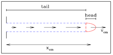
Fig. 1 Schematic diagram showing the structure of a “head/tail plasmon” produced by a single pulse ejection velocity variability. The rising velocity wing of the ejection pulse piles up into the leading head, and part of the decreasing velocity wing fills up the region between the head and the outflow source. The color figure can be viewed online. 

3.The Motion of the Plasmon Head

Under the assumption of a cylindrical flow, the position x_cm of the center of mass of the material that has entered the working surface at the head of the plasmon (see equation 1 of ^{Raga et al. 2020}) is given by:

where ρa is the (possibly position-dependent) environmental density, u₀(τ´) and ρ0(τ') are the ejection velocity and density (respectively), x_j is given by:

and the integration limit τ is the root of:

Following ^{Cantó et al. (2000)} and ^{Raga et al. (2020)}, instead of inverting equation (8), we will use τ (i.e., the ejection time) as independent variable, and find x_cm (from equation 6) and the evolutionary time t (from equation 8) as a function of τ.

We now consider a Gaussian ejection velocity variability (see equation 4), a constant ejection density p₀ and a uniform ambient density p_a. Equation (6) then takes the form:

where

and

is the error function.

From equations (9-10) we obtain the quadratic equation for x_cm:

with

4.Solutions for Different σ Values

4.2.Solutions for σ > 0

For σ > 0, the position x_cm of the head of the plasmon can be straightforwardly obtained by inverting equation (9), and evaluating the integrals (see equation 10) as a function of the ejection time τ. Also, calculating the evolutionary time t as a function of τ (see equation 8), we can obtain x_cm(t). Doing the appropriate time derivatives (analytically or numerically), we can also obtain the velocity v_cm = dx_cm/dt of the plasmon head.

The results obtained for different values of σ are shown in Figure 2. It is clear that for σ = 0 the plasmon reaches the asymptotic velocity v _a (see equation 18). For σ >0, v_cm, reaches a maximum value and then decreases as a funciton of time as the plasmon head incorporates more environmental material.

Fig. 2.  Dimensionlessposition (top) and velocity (bottom) of the plasmon head as a function of evolutionary time for σ = 0 (black curve), 0.1 (cyan), 1.0 (blue), 10 (red) and 100 (green). The solid curves show the results for the constant ejection density problem, and the dashed curves show the Gaussian ejection density case (with σ₁ values equal to the σ values given above). The color figure can be viewed online. 

For σ > 0, the head of the plasmon has a mass given by the contribution from the ejection pulse (see equation 19) and also a contribution from the environment:

Ma(τ)=M0 σ2xcm(τ)v0τ0 , (20)

where M₀ is the mass of the ejection pulse and σ is given by equation (13).

The mass in the tail (i.e., in the continuous beam segment between x = 0 and x_cm) is:

Mt(τ)=M02[erf(tτ0)-erf(ττ0)], (21)

In Figure 3 we plot the mass M_t of the tail, the total mass M_h = M_p + M_a of the plasmon head and the fraction M _a /M_h of this mass that corresponds to the swept-up environment as a function of the evolutionary time t for models with different σ values.

Fig. 3 Dimensionless mass (top) of the “constant density plasmon” head M_h (solid curves) and tail M_t (dashed lines), and fraction of environmental mass within the head (bottom). The results obtained for models with σ = 0 (black curves), 0.1 (cyan), 1.0 (blue), 10 (red) and 100 (green) are shown. The color figure can be viewed online. 

5.The Case of a Gaussian Ejection Density Variability

Let us now consider an ejection with a Gaussian velocity variability (see equation 4) and also with a Gaussian density variability:

of the same shape. In this equation, ρ0(τ) (in boldface) is the time-dependent ejection density, and p₀ is the peak density.

Inserting the ejection velocity (equation 4) and density (equation 22) variabilities into equation (6), we obtain an equation of the same form as (9), but with

Combining equations (9) and (23), we obtain the quadratic equation for x_cm:

with

The position x_cm and velocity dx_cm/dt as a function of 𝑡 obtained for different σ₁ values are shown in Figure 2. It is clear that for all σ₁ values, the plasmon head is faster than the “constant density plasmon” with σ = σ₁ (see equations 13 and 25). For σ₁ = σ > 0, the “Gaussian density” and “constant density” plasmons converge to the same velocity for t >> τ₀.

Also, using the appropriate integral from equation (23), we find that the contribution from the ejection pulse to the mass of the plasmon head as a function of τ is:

where M₀ is the mass of the ejection pulse. The mass in the tail (i.e., in the continuous beam segment between x = 0 and x_cm) is:

The head of the plasmon has a mass given by the contribution from the ejection pulse (see equation 28) and a contribution from the environment:

where M₀ is the mass of the ejection pulse and σ₁ is given by equation (25).

In Figure 4 we plot the mass M_t,1 of the tail, the total mass M_h,1 = M_p,1 + Ma_,1 of the plasmon head and the fraction M_a,1/M_h,1 of this mass that corresponds to the swept-up environment as a function of the evolutionary time t for models with different σ₁ values. The results are qualitatively similar to the ones obtained for the constant ejection density plasmon (see Figure 2).

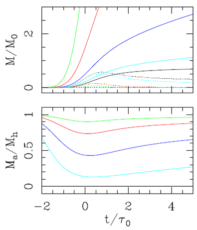
Fig. 4.  Dimensionlessmass (top) of the “Gaussian density plasmon” head M_h (solid curves) and tail Mt (dashed lines), and fraction of environmental mass within the head (bottom). The results obtained for models with σ₁ = 0 (black curves), 0.1 (cyan), 1.0 (blue), 10 (red) and 100 (green) are shown. The color figure can be viewed online. 

6.The Velocity and Density Structure of the Tail

We now calculate the density along the plasmon tail. To this effect, we use the solution to the continuity equation of a free-streaming, plane-parallel flow:

where u̇0(τ)=du0/dτ (see, e.g., ^{Raga & Kofman 1992}). For our Gaussian u₀(τ) (see equation 1) we then have:

where x, t and τ are related to each other through the free-streaming condition (equation 1).

In Figure 5, we show the free streaming velocity and density along the tail of the constant ejection density (see § 4) and Gaussian ejection density (§ 5) free plasmons (i.e., with σ = 0) for different evolutionary times. As shown by ^{Raga et al. (2020}, who studied a plasmon with a parabolic ejection velocity), for t > τ₀ the plasmon tail develops a “Hubble law” linear velocity vs. position dependence.

Fig. 5 Velocity (top) and density (bottom) vs. position along the plasmon tails, for evolutionary times t/ τ₀= 0, 1, 3, 5 and 7 (the curves are labeled with these times). The curves end in an open circle, which indicates the position (and in the top diagrams, the velocity) of the plasmon head. The results obtained for the constant ejection density case are shown in the left frames, and the ones obtained for the Gaussian ejection density on the right. The color figure can be viewed online. 

For both plasmon solutions, the density along the tail has its peak value approaching the position of the plasmon head (at all times shown in Figure 5). At t = τ₀, the constant ejection density plasmon tail has a second peak at x = 0, and develops a flat density vs. position structure at larger evolutionary times. At x = 0, the Gaussian ejection density plasmon has a density that → 0 at larger evolutionary times, leading to steeper density vs. position dependencies.

7.Summary

As a follow up to the paper of ^{Raga et al. (2020)}, who studied the flow resulting from an ejection velocity pulse with a parabolic time-dependence (and a time-independent mass loss rate), we consider ejection pulses with different time histories.

In particular, we study the flow resulting from a collimated ejection velocity pulse with a Gaussian time-dependence, considering the cases of a constant ejection density and a density with a Gaussian time-dependence (with the same width as the ejection velocity), moving into a uniform environment. Using the “center of mass formalism” of ^{Cantó et al. (2000)}, we derive full analytic solutions (given in terms of the error function) for both cases.

We calculate the position and velocity of the plasmon head as a function of time, and obtain very similar results for the constant and Gaussian ejection densities (Figure 2). The two cases produce an initial acceleration of the plasmon head, followed by a convergence to a constant velocity (for the σ = 0, “free plasmon” case) or by a gradual velocity decrease for cases with substantial environmental braking (i.e., for σ > 0).

We also calculate the mass in the head and tail of the plasmon as a function of evolutionary time. We find that:

Finally, we calculate the velocity and mass as a function of position for the σ = 0plasmons (see Figure 5). We recover the result of ^{Raga et al. (2020}) that for t > τ₀ the tail has a velocity structure that approaches a linear “Hubble law” velocity vs. position. For the density structure, we see that there is a peak just before the head of the plasmon. In the rest of the tail, there are substantial differences between the constant and Gaussian ejection density cases, with the former case having zero density at x = 0, and the latter case having a density ≈ 2 times lower than the peak density (at the position just before the head).

Therefore, we find that the assumption of a constant or a Gaussian time-dependent ejection density does not affect the dynamical characteristics of the “head/tail plasmon” in a substantial way. The main differences between these two cases are the mass and the density distribution within the plasmon tail.

We should note that the dynamical characteristics of the plasmons studied in this paper are also very similar to the ones of the “parabolic velocity pulse” plasmon studied by ^{Raga et al. (2020)}. From this, we conclude that at least at large evolutionary times (i.e., for t > τ₀) the dynamics of the head/tail plasmon are mostly independent of the details of the velocity and density ejection histories. The only important effect of different forms of the ejection is to change the mass content and density stratification of the material in the plasmon tail.

Now, the way forward to study the head/tail plasmon flow is with full axisymmetric or 3D numerical simulations of the flow. This will allow, among other things, an evaluation of the observational characteristics of the flow and of the stability of the plasmon head at large evolutionary times. Also, it would be interesting to extend the present work to the relativistic case, since it would have clear applications to microquasars and gamma-ray bursts.