SciELO - Scientific Electronic Library Online

 
vol.57 número1New Spectral Analysis Results Within the Scope of Extended Matter Research in the AR Lacertae Active Binary SystemArtificial Neural Network Modeling of the Conformable Fractional Isothermal Gas Spheres índice de autoresíndice de materiabúsqueda de artículos
Home Pagelista alfabética de revistas  

Servicios Personalizados

Revista

Articulo

Indicadores

Links relacionados

  • No hay artículos similaresSimilares en SciELO

Compartir


Revista mexicana de astronomía y astrofísica

versión impresa ISSN 0185-1101

Rev. mex. astron. astrofis vol.57 no.1 Ciudad de México abr. 2021  Epub 30-Sep-2021

https://doi.org/10.22201/ia.01851101p.2021.57.01.13 

Articles

Analytic Solutions for Truncated Plasmons

J. Cantó1 

A. C. Raga2  3 

1Instituto de Astronomía, UNAM, México.

2Instituto de Ciencias Nucleares, UNAM, México.

3Inst. de Investigación en Ciencias Físicas y Matemáticas, USAC, Guatemala.


ABSTRACT

We present a new plasmon model for a cometary clump moving supersonically in an environment with a non-zero gas pressure. We find that the environmental pressure produces a cutoff in the wings of the cometary clump, therefore resulting in quite \stubby" plasmons for a large range of ow Mach numbers. We derive a relation between the length-to-width ratio of the plasmon and the Mach number M of the ow, which could be used to directly derive M from observations of (appropriate) cometary clumps.

Key Words HII regions; ISM; jets and outows; ISM; kinematics and dynamics; planetary nebulae; general; shock waves

RESUMEN

Presentamos un nuevo modelo de plasmón para un nudo cometario moviéndose supersónicamente respecto de un medio ambiente con presión finita. Encontramos que la presión del medio ambiente produce un corte en las alas del nudo cometario, dando como resultado nudos \rellenitos" para un gran intervalo de números de Mach del flujo. Derivamos una relación entre el cociente \largo a ancho" del plasmón y el número de Mach M del flujo, el cual podría ser usado para derivar directamente M de observaciones de nudos cometarios apropiados.

1.Introduction

De Young & Axford (1967) derived the so-called “plasmon” solution, which consists of the balance between the gas pressure within a decelerating (or accelerating) isothermal clump of gas and the ram-pressure of the environment into which it is travelling. This simple solution still continues to be used to model the dynamics of different astrophysical flows involving cometary clumps (see, e.g., Rivera-Oríz et al. 2019a, b; Veilleux et al. 1999; De Young 1997).

Modified versions of the plasmon solution of De Young & Axford (1967) have been obtained including the effects of:

The formation of “tails” by wind/clump interactions was explored analytically by Dyson, Hartquist & Biro (1993).

Numerical simulations show that plasmon-style “interstellar bullet” flows are highly unstable, with rather intense fragmentation of the plasmon configuration (see, e.g., Klein et al. 2003; Raga et al. 2007). It can be argued that if a high speed flow rapidly disrupts a liquid droplet (see, e.g., Nicholls & Ranger 1969), a gas cloud would be disrupted with even greater ease.

On the other hand, it is clear that some astrophysical flows (e.g., the Orion “fingers” around the BN-KL object, see Rivera-Ortíz et al. 2019a) do show the characteristics predicted by the “braking plasmon” analytic model. In a recent series of papers, Pittard et al. (2009, 2010) and Goldsmith & Pittard (2017, 2019) show that clumps with high clump to environment density ratios can be substantially braked (or accelerated, depending on the reference system) before fragmenting and mixing with the environment. This “dense clump regime” was also explored by Rivera et al. (2019b), who carried out a comparison between an analytic plasmon model and numerical simulations. At least for such dense gas clumps, it appears that the plasmon model of De Young & Axford (1967) is still relevant.

In the present paper we consider the effect of the environmental gas pressure on the structure of a plasmon. This pressure will of course have an important effect for a plasmon moving at a relatively low Mach number (with respect to the environmental sound speed). Also, even in the case of a high Mach number plasmon, the environmental pressure will have an important effect in the plasmon “wings”, where the bow shock becomes highly oblique.

The paper is organized as follows. In § 2, we present the new plasmon model, and derive a full analytic solution for the shape of the plasmon. In § 3 we derive the equation of motion for the modified plasmon, and integrate it numerically to determine the velocity and position of the plasmon as a function of time. Finally, we present a discussion of the results in § 4.

2.The Plasmon Model

We consider the situation shown in the schematic diagram of Figure 1. In a cylindrical reference frame moving with the plasmon, the surrounding environment (of density ρa, pressure P a and isothermal sound speed ca=Pa/ρa) impinges on the plasmon with a velocity v a (this is the relative velocity between the environment and the plasmon).

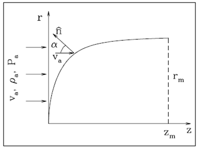
Fig. 1 Schematic diagram of a plasmon. In a frame of reference at rest with the plasmon, the environment (of density ρa and pressure P a ) impinges from the left, along the symmetry axis of the (z,r) cylindrical coordinate system. The thick curve represents the surface of the plasmon, which is truncated at the position (zm, rm). We show the angle α between the direction of the impinging flow and the local normal to the plasmon surface. 

In our model, we assume that the environment is isothermal, with a position-independent sound speed c a . We also assume that the plasmon is isothermal, but allow it to have a different sound speed c0. This choice is appropriate for a dense clump in an outflow from a young star, travelling within a higher temperature, neutral or partially ionized environment.

We assume that at any time in its evolution, the internal pressure stratification of the decelerating (or accelerating) plasmon instantaneously relaxes to the hydrostatic equilibrium, so that:

P(z)=P0e-z/H, (1)

for an isothermal gas, where

Hc02a, (2)

with c0 being the isothermal sound speed and α the acceleration/deceleration of the plasmon. An exploration of the validity of equation 1 is presented in Appendix B.

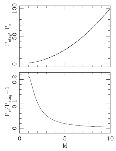
As discussed in Appendix A, the pressure of the shocked environment in contact with the plasmon is approximately given by:

Ps=Pa+ρava2cos2α, (3)

where ρa, v a and P a are the ambient density, velocity and pressure (respectively) and α=arctan(dz/dr) is the angle between the impinging flow and the normal to the surface of the plasmon (see Figure 1). Therefore, the pressure P0 at the head of the plasmon (see equation 1) is:

P0=(1+β)ρava2, (4)

with

βPaρava2=1M2, (5)

where M is the Mach number calculated with the velocity v a of the plasmon and the isothermal sound speed c a of the environment.

Now, setting P(z)=Ps (equations 1 and 3) and considering that dz/dr = tan α (see Figure 1), we obtain the differential equation

dzdr=tanα=1(1+β)e-z/H-β-1, (6)

with β given by equation (5).

From the second equality of equation (6) we obtain:

z=Hln(1+β)(1+ω)1+β(1+ω), (7)

with

ω=tan2α. (8)

It is clear that the plasmon solution ends at a finite zm, for which α=π/2 (so that also ω=tanα). From equation (7) we obtain:

zm=Hln1+ββ. (9)

In order to obtain the z(r) solution, we first consider the first equality of equation (6):

dr=dzω, (10)

where ω is defined in equation (8). Also, from equation (7) we have:

dz=H(1+ω)1+β(1+ω)dω. (11)

Combining equations (10-11) we obtain the differential equation:

drdω=H(1+ω)1+β(1+ω)ω, (12)

which can be integrated to obtain:

r=2Htan-1ω-β1+βtan-1βω1+β, (13)

with ω given by equation (8). Equations (8) and (13) are then the solution for the shape of a plasmon interacting with an environment with a non-zero gas pressure.

This solution has the following limiting cases:

z1

r2zH1+β, (14)

zzm (see equation 9):

rrm=πH1-β1+β, (15)

β0

r=2Htan-1ez/H-1. (16)

Equation (16) is the plasmon solution of De Young & Axford (1967).

In Figure 2, we plot the r(z) solutions (equations 8 and 13) for different values of β. It is clear that the length-to-width ratio of the plasmon grows as a function of decreasing β. This effect can be quantified by calculating the length-to-width ratio L/W=zm/(2rm) from equations (9) and (15):

L/W=12πln1+ββ1-β1+β=12πln1+M21-11+M2, (17)

where for the second equality, we have used the M2=1/β relation. This Mach number dependence of the length-to-width ratio of the plasmon is shown in Figure 3.

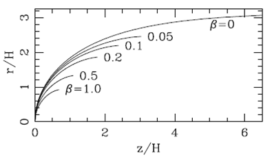
Fig. 2. The plasmon solution for different values of β. The curves are labeled with the corresponding β values. 

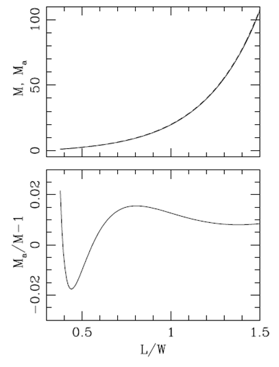
Fig. 3. Topplot: Mach numbers M (from the “exact” equation 17) and M a (from the approximate inversion 18) as a function of the length-to-width ratio of the plasmon. Bottom plot: relative error of the approximate inversion as a function of L/W. 

It is of interest to have an analytic expression for calculating the Mach number M of the plasmon flow as a function of the observed L/W length-to-width ratio. As equation (17) does not have an analytic inversion, we propose the fit:

Ma=π3/2eπ(L/W)(L/W)-1.5+5.18-0.16. (18)

In Figure 3, we also show M a vs. M/L solution, as well as its relative deviation (Ma-M)/M (with M given by equation 17) with respect to the exact solution. In the bottom frame of Figure 3, we see that for the M=1100 Mach number range, the relative error of the interpolation of equation (18) is smaller than 2%.

Finally, we calculate the mass of the plasmon. To do this, we combine equations (1), (4) and (8) to obtain

ρ(ω)=ρ01+β(1+ω)(1+β)(1+ω), (19)

with ρ0=P0/c02 being the density at the head of the plasmon. Now, using equations (19), (11) and (13) we can calculate the mass Mp of the plasmon:

Mp=π0zmρ(z)r2dz=4πρ0H3m(β), (20)

with

m(β)=0tan-1ω-β1+βtan-1βω1+β2(1+β)(1+ω)2dω. (21)

We have not been able to carry out this integral analytically. However, in the limits of low and high β one obtains:

m(β)π2-48-3π2-48β;β1, (22)

m(β)=9π2-161921β3;β1. (23)

This latter, β >> 1, limit corresponds to a highly subsonic flow, for which our model is probably not appropriate.

A good analytic approximation for β in the full 0 range is:

ma(β)=b01+b1β+b2β2+b3β3, (24)

with

b0=π2-48;b1=3π2-4π2-4;b2=5.25367;b3=24(π2-4)9π2-16. (25)

Figure 4 (top) shows the dimensionless mass m obtained from a numerical integration of equation (21) as a function of β, as well as the analytic approximation m a . The bottom plot shows the relative deviation between these two solutions, and we can see that the approximate analytic solution has deviations of less that 3% relative to the exact (i.e., numerical) solution.

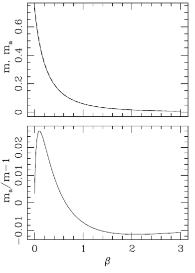
Fig. 4. Topplot: Dimensionless mass m (solid line, obtained from a numerical integration of equation 21) and the approximate solution m a (dashed line, from equation 24) as a function of β =1/M2 (where M is the Mach number of the flow). Bottom plot: relative error of the approximate, analytic solution as a function of β. 

3.The Equation of Motion for the Plasmon

The plasmon’s equation of motion can be straightforwardly derived noting that the deceleration of the plasmon is a=c02/H (see equation 2), and then writing H in terms of the plasmon mass using equation (20). We then obtain:

a=dvadt=-4πρac04(1+β)va2m(β)Mp1/3, (26)

where we have also used equation (4). We note that in this equation, β=ca2/va2.

Equation (26) was derived assuming that the plasmon has a time-independent mass. This is of course not necessarily true, since

  1. the plasmon could evaporate from the back side (which is probably not an important effect in the pressure confined plasmon tail that we are modelling here),

  2. the flow around the plasmon head could entrain a substantial amount of plasmon material.

A parametrization of the “detrainment” of material from a plasmon has been obtained by Rivera-Ortíz et al. (2019b) by comparing a mass-losing plasmon analytic model with numerical simulations. Through their combined analytic and numerical aproach, these authors estimate a characteristic timescale

tm=10.45Hc0 (27)

for substantial mass loss from the plasmon. A mass conserving plasmon model is therefore appropriate only for evolutionary times <tm.

We first define dimensionless variables:

x'=xl0;v'=vaca;t'=tcal0, (28)

where x is the position of the plasmon, and

l0Mp4πρa1/3cac04/3. (29)

In terms of these dimensionless variables, equation (26) takes the form:

d2x'dt'2=dv'dt'=-1+v'2m1v'21/3. (30)

This is the equation of motion for the plasmon, and a numerical integration is presented in § 3.

For v'1, we can set 1+v'2v'2, and

m(1/v')b0=π2-48, (31)

(see equation 22 and 25) in the second equality of equation (30). With an initial condition (the initial Mach number of the plasmon), we integrate this equation to obtain:

v'(t')=M01/3-b01/3t'33. (32)

It is clear that v'0 as t't'0, with

t'03M0b01/3. (33)

We can integrate again to obtain the dimensionless position of the plasmon as a function of time:

x'(t')=3M04b01/31-1-b01/3t'3M01/34, (34)

where we have assumed that x'(t'=0)=0. This solution has been previously derived, e.g., by Cabrit & Raga (2000).

In Figure 5 we present a comparison of the “large Mach number” analytical solution (equations 32 and 34) with a full, numerical integration of equation (30) for a plasmon with a v'(t'=0)=M0=10 initial Mach number. It is clear that initially the two solutions are most similar, and that they start diverging when the plasmon slows down to v'1. While the analytic, high Mach number solution (which is really not applicable in this low v´ regime) shows a plasmon which stops at a time t0 (see equation 33), the full solution gives a plasmon that gradually slows down but does not stop at a finite distance.

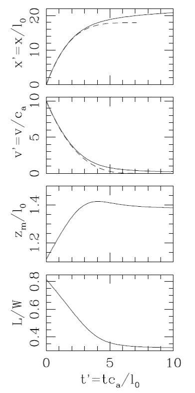
Fig. 5 Dimensionless position (top) and velocity (second from top) as a function of time. The solid curves correspond to the full (numerical solution of equation (30), and the dashed curves to the “high Mach number” analytic solution (equations 32 and 34). The two bottom frames show the dimensionless axial extent zm/l0 and the length-to-width ratio L/W of the plasmon as a function of time. 

Figure 5 also shows the axial extent zm (equation 9) and the length-to-width ratio (L/W, given by equation 17) of the plasmon as a function of time. The length zm initially grows with time, reaches a peak (of ≈1.42l0) and then slowly decreases for times t>4l0/ca. The length-to-width ratio decreases monotonically from a L/W≈0.8 down to an asymptotic value of ≈0.32.

4.Discussion

We have derived an analytic solution for the problem of an isothermal plasmon travelling supersonicaly within an environment with a non-zero pressure.

For a hypersonic flow with M >>1, our model coincides with the De Young & Axford (1967) plasmon solution.

Interestingly, we find that even for large values of M the non-zero environmental pressure produces a cut-off for the plasmon, which is terminated at the distance zm and cylindrical radius rm from the plasmon head given by equations (9) and (15). Thus cutoff results in rather stubby plasmons (see Figure 2), unless one goes to very high Mach number flows.

We find that the length-to-width ratio of the plasmon solution (equations 17 and 18) has values ranging from ≈0.4 to ≈1.5 for Mach numbers M=1100 (see Figure 3). Therefore, the extended wings of the De Young & Axford (1967) solution will basically never be formed in a real astrophysical flow, unless it has an extremely high Mach number. We find an analytical expression (equation 18) that can be used to derive an estimate for the flow Mach number from the observed length-to-width ratio of a cometary clump.

We also integrated the equation of motion for the new plasmon solution, and for high Mach numbers we find (not surprisingly) a time-dependent position and velocity which are similar to the ones found from the De Young & Axford (1967) plasmon solution. When the flow reaches a Mach number of ≈3, the new solution starts to separate from the De Young & Axford model, with the plasmon slowing down more slowly, and never stopping completely (while the De Young & Axford plasmon stops at a finite distance along its direction of motion).

Finally, we would like to point out an important qualitative result obtained from our new model. The ratio between the extent along the symmetry axis of the plasmon zm and the scale-height H (equation 9) only has a logarithmic dependence on β=1/M2 (see equation 5). Therefore, for a wide range of possible values of M a , we will have H ≈zm, so that the gas within the plasmon will not be strongly stratified (as for this, one would need many pressure scale heights fitting within the length of the plasmon). This is a feature that is found when one tries to fit clumps obtained in numerical simulations with an analytic plasmon solution (see, e.g., Raga et al. 1998).

Acknowledgements

This work was supported by the DGAPA (UNAM) grant IG100218. We acknowledge an anonymous referee for helpful comments which (among other things) lead to the discussion in Appendix B.

References

Cabrit, S. & Raga, A. C. 2000, A&A, 354, 667 [ Links ]

Cantó, J. & Raga, A. C. 1995, MNRAS, 277, 1120 [ Links ]

Cantó, J., Espresate, J., Raga, A. C., & D’Alessio, P. 1998, MNRAS, 296, 1041 [ Links ]

de Young, D. S. 1997, ApJ, 490, 55 [ Links ]

de Young, D. S. & Axford, W. I. 1967, Natur, 216, 129 [ Links ]

Dyson, J. E., Hartquist, T. W., & Biro, S. 1993, MNRAS, 261, 430 [ Links ]

Goldsmith, K. J. A. & Pittard, J. M. 2017, MNRAS, 470, 2427 [ Links ]

______2018, MNRAS, 476, 2209 [ Links ]

Klein, R. I., Budil, K. S., Perry, T. S., & Bach, D. R. 2003, ApJ, 583, 245 [ Links ]

Lora, V., Raga, A. C., & Grebel, E. K. 2015, RMxAA, 51, 41 [ Links ]

Nicholls, J. A. & Ranger, A. A. 1969, AIAAJ, 7, 285 [ Links ]

Pittard, J. M., Falle, S. A. E. G., Hartquist, T. W., & Dyson, J. E. 2009, MNRAS, 394, 1351 [ Links ]

Pittard, J. M., Hartquist, T. W., & Falle, S. A. E. G. 2010, MNRAS, 405, 821 [ Links ]

Raga, A. C., Cantó, J., Curiel, S., & Taylor, S. 1998, MNRAS, 295, 738 [ Links ]

Raga, A. C., Esquivel, A., Riera, A., & Velázquez, P. F. 2007, ApJ, 668, 310 [ Links ]

Rivera-Ortíz, P. R., Rodríguez-González, A., Hernández-Martínez, L., Cantó, J., & Zapata, L. A. 2019a, ApJ, 885, 104R [ Links ]

Rivera-Ortíz, P. R., Rodríguez-González, A., Hernández-Martínez, L., & Cantó, J. 2019b, ApJ, 874, 38R [ Links ]

Veilleux, S., Bland-Hawthorn, J., Cecil, G., Tully, R. B., & Miller, S. T. 1999, ApJ, 520, 111 [ Links ]

Appendices

A.The pressure on the surface of the plasmon

In § 2, we have assumed that the pressure of the shocked environment at the surface of the plasmon is

Ps=Pa+ρav2, (A35)

where ρa and Pa are the pre-shock density and pressure (respectively) and v is the component of the pre-shock flow normal to the shock surface, see equation (3). This equation can be written as:

Psρaca2=M2+1, (A36)

where M=v/ca is the Mach number calculated with the normal velocity and the isothermal sound speed.

This form for the pressure on the plasmon has the desired behaviour so that when the surface of the plasmon becomes parallel to the direction of the impinging flow (and therefore the normal velocity is v0), the pressure on the plasmon is equal to the environmental gas pressure Pa. It is not clear whether or not equation (A35) gives the correct pressure for other orientations of the flow relative to the impinging flow.

To illustrate the kind of accuracy we obtain when using equation (A35), let us consider the stagnation region, where the environment flows normal to the plasmom surface (see Figure 1). For an isothermal shock, the postshock velocity v p and the density ρp are given by:

vp=ca2va;ρp=vacaρ, (A37)

where c a is the isothermal sound speed of the flow, and v a and ρa are the preshock velocity and density (respectively). After going through the shock, the material slows down, until it is at rest at the stagnation point in contact with the head of the plasmon. The conditions at the stagnation region can be calculated with the isothermal Bernoulli theorem, giving the relation

vp22+ca2lnρp=ca2lnρstag, (A38)

where ρstag is the density at the stagnation point. Using equations (A37-A38) we can calculate the stagnation pressure

Pstagρaca2=M2e1/(2M2), (A39)

with M=va/ca.

The value of Pstag obtained from equation (A39) clearly does not coincide with the pressure on the head of the plasmon calculated with equation (A35) or (A36). In order to show the differences between these two pressure values, we plot the two of them (as well as their relative difference) as a function of Mach number M in Figure 6. We see that the pressure obtained from equation (A36) differs from the correct stagnation pressure (given by equation A39) by ≈ 22% for M=1, and that it has smaller deviations for increasing values of M.

Fig. 6 Top frame: the Ps (dashed curve) and Pstag (solid curve) pressures (obtained from equations A36 and A39, respectively) as a function of pre-shock Mach number M. Bottom frame: the relative deviation (Ps -Pstah)/Pstag between the two pressures as a function of M. 

From this, we conclude that the pressure on the plasmon surface given by equation (A35) has an accuracy that is appropriate for the simple, analytic plasmon model derived in our paper.

B.The Assumption of a Hydrostatic Stratification

Following De Young & Axford (1967), we have assumed that the plasmon has a hydrostatic equilibrium internal pressure distribution (see equation 1). This assumption is valid provided that the timescale τa for changes in the acceleration (or deceleration) 𝑎 is smaller than the sound crossing time of the plasmon:

τhb=zmc0=c0aln1+ββ, (B40)

where zm is the axial extent, c0 the sound speed and β=(ca/v)2 (see equations 2, 5 and 9).

In order to estimate the timescale

τa=ada/dt (B41)

for substantial changes in the acceleration we first note that equation (30) can be written in an approximate way as:

a=dvdtAv2/3, (B42)

where A is a constant and we have assumed and vca. Taking the time derivative of this equation, we obtain:

τa32τv;  with τv=vdvdt=va, (B43)

where τv is the timescale for changes in the plasmon velocity v.

Finally. combining equations (B40) and (B43), we find that the condition for hydrostatic balance within the plasmon can be written as:

τhbτac0caf(v')<1, (B44)

wiht v'=v/ca and

f(v')=23v'ln1+v'2. (B45)

This function is shown in Figure 7, in which we see that it has a maximum value f(v'p)=0.536 at v'p=1.981. Therefore, the hydrostatic balance within the plasmon will be satisfied over all of its deceleration history for the case of a “cold plasmon” with c0<1.8ca (where c0 and c a are the isothermal sound speeds of the plasmon and of the environment, respectively).

Fig. 7 The f(v/c a ) function of the criterion for hydrostatic balance within the plasmon, see equations (B44-B45). 

Received: July 23, 2020; Accepted: November 19, 2020

Creative Commons License Este es un artículo publicado en acceso abierto bajo una licencia Creative Commons