


 nueva página del texto (beta)
 Inglés (pdf)
 Artículo en XML
 Referencias del artículo
 Enviar artículo por email
 Citado por SciELO
  Similares en
SciELO
Similares en
SciELO 
 Permalink
1.Introduction
Wolszczan and Frail studying the radio pulsar PSR1257+12 deduced the presence of two orbiting Earth-mass bodies : this was the first widely-accepted discovery of an exoplanet. Later, in 1995, Mayor and Queloz, using the radial velocity method, discovered the first exoplanet orbiting a solar type star, 51 Peg . With this latter discovery began an entirely new field of astronomy: the study of exoplanets. So far, applying different observational methods the number of confirmed exoplanets has reached 4276 (https://exoplanetarchive.ipac.caltech.edu, september 2020). These observations have given us new insight on the extraordinary diversity of exoplanetary systems in our Milky Way (planets are found with very different masses, sizes and spatial distributions).
Among the available methods used to detect and characterize exoplanets, two techniques appear to be most effective: the transit photometry and the radial velocity. First, the transit photometric method, which is especially efficient, is used to detect tiny decreases (1 to 100 ppm) of the luminosity in the light curve of the central star. These correspond to the primary (transit) and secondary (occultation) star-planet eclipses. It allows us, in particular, to obtain an estimation of the planet’s radius. Second, also when the star´s orbit is inclined, the star exhibits a periodic Doppler shift, so that in the stellar spectrum we are able to measure the blue and red shifted lines and, therefore, to estimate the star radial velocity curve. This is the so-called radial velocity method that allows us to obtain an estimation of the planet’s mass. Combining these two methods provides a better characterization of an exoplanet.
Also, high-precision photometry from the Kepler mission has enabled us to study small-scale variable photometric effects that arise from the exoplanet motion around its host star; for example, stellar brightness also varies between eclipses due to three photometric effects that are: reflected light (as planetary contribution to the system light curve), the ellipsoidal variations (tidal ellipsoidal distortion) and the Doppler beaming (arising from modulation of the stellar flux by interactions with the orbiting planet). The magnitude of these effects is very weak, commonly, less than 100 ppm (Loeb & Gaudi 2003). Until the launch of CoRot and Kepler telescopes, the precision required to study these small-scale interactions was not available.
The photometric variation of the light curve due to these three effects, without considering the eclipses, is referred hereafter as the planetary phase curve. An important advantage of phase curve analysis is that it permits a full characterization of the physical and orbital parameters of an exoplanet. Several groups have been working in this way, characterizing individual exoplanets from their phase curves, e.g., planets discovered by the CoRot telescope, like CoRot-1b (Snellen et al. 2009) and planets discovered by the Kepler telescope like KOI-13b (Shporer et al. 2011; Mazeh et al. 2012), TrEs-2 (Barclay et al. 2012; Kipping & Spiegel 2011), Kepler-41b (Quintana et al. 2013), HAT-P-7b (Mislis et al. 2012; Welsh et al. 2010; Van Eylen et al. 2012), Kepler-6b, Kepler-8b studied by Esteves et al. (2013), who also studied the phase curves for some of the above mentioned planets focusing on those planets with a ratio
Regarding the Doppler beaming effect, it is the result from the reflection movement of a host star due to the interaction with an orbiting companion. In the composite phase curve, considering all photometric effects, the introduction of the beaming effect yields asymmetries in the whole pattern due to the sinusoidal variation.
In this contribution, we do not estimate the mass of the planet, although it could be done in a simple way. Instead, we focus on evaluating the Doppler beaming effect over each of all confirmed exoplanets, discovered so far by the Kepler telescope. In this way, we derive the planet radial velocity only for those planets which exhibit Doppler luminosity variations greater than 1 ppm. The Doppler beaming effect and the radial velocity for the selected planetary systems were theoretically evaluated using the parameters given in Table 1. In addition, they were also estimated from the observational data (experimental phase curve) using a fitting model. Finally, the obtained radial velocity values were compared with those found in the literature.
TABLE 1 EXOPLANET PARAMETERSa
| Kepler Exoplanet | Orbit period P (days) | Orbit inclination i | Planet mass Mp (Mj) | Steller temperature (K) | Stellar mass (Msun) |
|---|---|---|---|---|---|
| HAT-P7 | 2.204 | 83.14 | 1.78 | 6350 | 1.47 |
| Kepler-423b | 2.68 | 87.828 | 0.595 | 5560 | 0.85 |
| Kepler-5b | 3.55 | 89.14 | 2.11 | 6297 | 1.37 |
| Kepler-75b | 8.88 | 89.12 | 10.1 | 5200 | 0.91 |
| Kepler-8b | 3.522 | 83.978 | 0.59 | 6213 | 1.21 |
| 1.72KOI-13b | 1.763 | 83.77 | 9.28 | 7650 | 1.72 |
| Tr-ES-2b | 2.470 | 83.87 | 1.19 | 5850 | 0.98 |
aPublished values (http://exoplanetarchive.ipac.caltech.edu).
2.Phase Curve Modeling
Loeb & Gaudi (2003) have demonstrated that the small photometric variations of the phase curve arise from three different effects: the reflection and/or emission, the ellipsoidal and the Doppler beaming effect. Since the reflection and the planet thermal emission are degenerate at low eccentricities, these two planetary effects are difficult to distinguish. For this reason, both effects are added and considered hereafter together as only one planetary effect; the reflection effect, sometimes called the phase function. The first two effects vary as
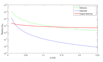
Fig. 1 Small scale photometric variations of a phase curve as a function of the radial semi-mayor axis of the planet orbit. The color figure can be viewed online.
In what follows, we describe these three effects denoting the mass and radius of the star, Sun, planet and Jupiter as: M*,R*, Msun, Rsun, Mp, Rp, Mj, Rj, respectively. The period of a planetary orbit is denoted by Porb, a and i are the semi-major axis of the planet orbit and its inclination with respect to the observation plane. Vr and K are the radial velocity and the semi-amplitude of the radial velocity and G and c are the gravitational constant and the speed of light.
2.1.Reflection Effect
This photometric effect, in essence, is an atmospheric phenomenon rather than a gravitational one. It mainly depends on the planet reflective capability. When a planet has a large albedo and is orbiting around a luminous star, its light variations are easier to detect in the visible range. Although the effect is small, it is significant for short-period planets in close orbits around their host stars. This is directly related to the fact that the stellar flux received by the planet decreases with distance as
Following the model described in Mazeh et al. (2012), Sudarsky et al. (2005) and Burrows & Orton (2009), the normalized photometric flux variation due to reflection is given by:
where the amplitude for the reflection effect, including the planetary thermal emission, is expressed as :
or in ppm units:
Here,
The amount of reflected light does not change during their orbit for planets with circular face-on orbits from Earth’s point of view; therefore, their reflected radiation is not detected.
In summary, planets in close orbits around their host star, larger planets, and planets with higher albedo, are easier to detect as they reflect more light.
2.2.Ellipsoidal Effect
The ellipsoidal effect has its origin in the gravitational deformation of the host star by an orbiting planet (tidal distortion). Planetary gravitational tidal forces produce stellar distortions that cause photometric variations of the light curve of exoplanetary systems. This effect was presented by Loeb & Gaudi (2003) and Drake (2003). Pfahl et al. (2008) provide a detailed theoretical investigation of the ellipsoidal deformation of the host star.
Following Morris (1985), we describe the flux variation of the light curve due to the ellipsoidal effect. He proposed a model for the normalized flux variation that includes the first three cosinusoidal harmonics of the phase angle φ(t), as follows:
The ellipsoidal variations are a gravitational effect which produces a double peak of equal height at the quarter phases of the orbit, contributing to an overall bi-modal feature in the light curve. Then, the tidal ellipsoidal normalized flux variation can be modulated in a cosinusoidal manner as:
where the ellipsoidal amplitude is given by Shporer et al. (2011):
or, in ppm units:
Mp, M* are the planetary and stellar masses, a, Porb and 𝑖 are the semi-major axis, period and inclination of the planetary orbit, respectively.
The effect of the stellar ellipsoidal distortions on the light curve can be larger than the relativistic beaming effect, which is often small, but the variation of the phase curve component is twice as fast. Furthermore, as seen in the relationships for calculating the ellipsoidal amplitude, the gravitational distortion of the star by the planet is larger if it has a low semi-major axis to stellar radius ratio and the density of the star is low. So, this ellipsoidal method can be used efficiently to find planets in evolved stars outside the main sequence. In contrast, the ellipsoidal effect is negligible for low mass planets far from the host stars.
2.3.Doppler Beaming Effect and Radial Velocity Estimation
The first theoretical contribution was presented by and the first observational contribution by Hills & Dale (1974) and the first observational contribution by Maxted et al. (2000). Loeb & Gaudi (2003) were first to present the photometric effect in the context of exoplanet characterization. As the star and planets are orbiting around the system’s barycenter, the host star will periodically advance toward, and recede from, an observer. Thus, the brightness of the host star will vary sinusoidally at the orbital frequency of the planet (a stellar wobble is induced by the planet). Then, as the star moves toward an observer, there is an increase in the observed flux, and as it recedes the observed flux decreases. It varies with the period of the orbit, but is off by a phase from the reflected light, since the maximum boosting occurs when the planet is in its first quarter phase and the star is moving toward the observer. The relativistic Doppler beaming (boosting), now is a detectable photometric variation effect, thanks to the high-precision photometry of space telescopes like Kepler (down to ≈10 parts per million). It is not an ideal method for discovering new planets, since the effect is small, even smaller than the emitted and reflected starlight from the planet. However, with the light variations due to relativistic beaming, it is easier to detect massive planets near their host stars, since these factors increase with the movement of the star (due to the motion around the center of mass of an exoplanet system). Like the radial velocity method, this can be used to determine the orbital eccentricity and the minimum mass of the planet (which is impossible to do from reflected light alone); but the Doppler beaming effect does not require a spectrum of the star, so it can be used to study more distant stars.
The Doppler beaming effect (DBE) itself has two contributions: the first one is actually the same Doppler beaming effect which increases the luminosity toward the direction of the radial velocity of the star. The second one is the Doppler shift of the star spectrum in the Kepler observation band. These two effects could be described by the following equations (Rybicki & Lightman 1979). First, considering a spherical star that radiates isotropically (or nearly isotropically) in the particle rest frame, the relativistic transformation of the received bolometric flux is given by:
where
where
Or, considering that
This relation, in this work, is evaluated using the well-known physical parameters, to make an analytical estimation of the radial velocity.
From here, the normalized flux variation for the Doppler beaming effect can be written as (Loeb & Gaudi 2003; Shporer et al. 2011)
where the beaming amplitude is found to be (Shporer et al. 2011):
Therefore, the amplitude of the effect can be used to estimate the mass of the planet if the host star mass is known. The amplitude of the observed Doppler beaming photometric variation depends on the bandpass through which the planetary system is observed. The actual value of
It is worth noting that the radial velocity can be estimated from the Doppler beaming amplitude. Therefore, the mass of the planet also can be estimated from the amplitude of the Doppler boosting, as this effect is proportional to the radial velocity. Finally, it is also important to keep in mind that the Doppler variations for short period (
3.Kepler Planetary Systems
We analyze all the quarters of the Kepler short and long cadence data for all the planets which exhibit a phase curve.
We start by computing the Doppler beaming effect, explained in § 2.3, for all confirmed exoplanets observed by the Kepler telescope (2776 objects). For that, we use the published data available at https://exoplanetarchive.ipac.caltech.edu. We found just 60 objects in which a Doppler beaming amplitude is detectable. Currently, the Kepler photometric instrument is sensitive enough to detect Doppler variations equal or greater than 1 ppm; this was not possible in past space missions.
During the mission, Kepler took 30 seconds short cadence (SC) integrations with its 42-CCD photometer (Borucki et al. 2010). For each exoplanet system, 10 to 50 photometric measurement files are available, corresponding to observations from 2009 to 2019. Details of the process of data reduction are explained below.
3.1.Removal of Systematics
First, in order to improve the signal to noise ratio, we treat the photometric data eliminating the jumps between the quarters and correcting for systematics. Since photometric variations are normally small for the primary and secondary eclipses, and even less between eclipses (due to the above mentioned photometric effects), we do not expect to have abrupt signal changes in the observed data. Then, in each data file a central moving median and a central moving average have been applied to eliminate bad points and to smooth the curve. We tested different combinations of these two steps, using 3 to 101 points, looking for the most suitable combination to smooth the curve without affecting the particularities of the signal (primary eclipse). A central moving median of 40 orders with a central moving average of 10 orders produced the best results. This procedure provided a light curve that had between 3 to 20 eclipses, depending on the planetary period and the available Kepler files. Finally, the phase curve for each planetary system was obtained by adding the light curve over parts of a period, applying the folding phase method. The phases φ = 0 in the primary eclipse and φ= π in the secondary, are taken as the starting points. The last step consists of removing the primary and secondary eclipses to obtain only the light variation curve between eclipses, which is the phase curve to be modeled.
Finally, we apply small-scale photometric variation models to find the best fitting curves to our observational data.
3.2.The Data Analysis: Phase Curve Fitting
The fitting model for a given light curve, essentially involves tuning the amplitude values for each of the three effects mentioned earlier, i.e., Arefl, AEllip, and ABeam, in order to find the best fit to the corresponding photometric data of our selected planetary systems.
As was shown in the previous section, the small-scale photometric variations of these planets are proportional to trigonometric functions of the phase φ which ranges from 0 to; 2π, 0 corresponds to the transit and 𝜋 to the occultation.
For the normalized phase curve, adding the contribution of all phase effects, the following expression describes the pattern for the relative flux variation:
A0 is expected to be of the order of unity, ABeam positive, ARefl and AEllip negative.
Only the planets with the correct amplitude effect (7 planets out of the original 60), have been presented in this work. The theoretical values for the amplitude ABeam have been obtained from the evaluation of the relations exhibited in the Phase Curve Modeling § 2, using the parameters (mass, radius, and inclination) given in Table 1.
In Figure 2, we present the composite phase curve for KOI-13b. For this planetary system the reflection contribution is dominant, but it is modulated by the bimodal ellipsoidal effect.

The Doppler beaming effect is also appreciable by the asymmetries in the total phase curve. However, the residual was not small enough to be considered as a good fit.
A result with a smaller residual (see Table 2) is obtained by incorporating, a priori, additional harmonics in 2φ and 3φ. Harmonics of higher order also have been considered, but no appreciable contributions was found.
TABLE 2 STANDARD RESIDUAL ERRORS FOR DIFFERENT MODELS
| Model 1: | Model 2: Model 1 | Model 3: Model 2 | |
| Three effects | +sin(2φ) | + 3φ term | |
| HAT-P-7b | 2.227e-06 | 1.953e-06 | 1.731e-06 |
| Kepler-423b | 2.075e-05 | 2.032e-05 | 1.99e-05 |
| Kepler-5b | 1.613e-05 | 1.602e-05 | 1.588e-05 |
| Kepler-75b | 0.0001155 | 0.0001146 | 0.0001141 |
| Kepler-8b | 2.663e-05 | 2.663e-05 | 2.662e-05 |
| KOI-13b | 4.458e-06 | 2.531e-06 | 1.116e-06 |
| TrES-2b | 3.28e-06 | 3.249e-06 | 3.229e-06 |
Therefore, the models described below have been applied to KOI-13 and the other planets of our selected sample (Figure 3):
Model 1: Reflection effect + DBE + Ellipsoidal effect
Model 2: Reflection effect + DBE + Ellipsoidal effect + sin(2φ)
Model 3: Reflection effect + DBE + Ellipsoidal effect + sin(2φ) + cos(3φ) + sin(3φ)
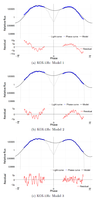
Fig. 3 KOI-13b planetary light curve, phase curve, fitting model, and residuals for each of the three models indicated in the text. The color figure can be viewed online.
In Figure 4 the phase curves with their best fitting models are presented for each of the six planetary systems that were analyzed in this contribution.
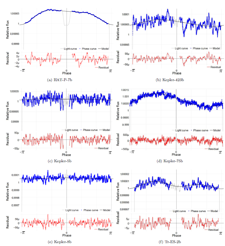
Fig. 4 Light curve, phase curve, fit model, and residual for the different planets we found with coherent effect sign. The color figure can be viewed online.
In Table 3 we show, together with the published values, the theoretical and estimated Doppler amplitudes ABeam, along with the values deduced for the radial velocity K.
TABLE 3 DOPPLER BEAMING AMPLITUDE AND RADIAL VELOCITY
| Kepler Exoplanet (ppm) | Theoretical ABeam a (m.s-1) | Theoretical Ka (ppm) | Calculated ABeam b (m.s-1) | Calculated Kb (ppm) | Published ABeam (m.s-1) | Published K |
|---|---|---|---|---|---|---|
| HAT-P-7b | 2.75 | 213.33 | 5.19 ± 1.99 | 402.43 ± 155.43 | 5.8 ± 0.19 3 | 211.8 ± 2.6 8 |
| Kepler-423b | 1.41 | 98.88 | 12.74 ± 2.36 | 873.36 ± 159.49 | NA | 96.7 ± 11.8 11 |
| Kepler-5b | 2.96 | 227.77 | 4.74 ± 3.22 | 366.84 ± 247.08 | NA | 227.5 ± 2.8 10 |
| Kepler-75b | 19.94 | 1283.04 | 384.4 ± 290 | 24731 ± 18575.44 | NA | 1288 ± 24 12 |
| Kepler-8b | 0.90 | 68.94 | 0:29 ± 26 | 2.5 ± 1.2 3 | NA | |
| KOI-13b | 11.85 | 1084.47 | 11.70 ± 4.2 | 1100.73 ± 376.02 | 7.14 ± 0.24 3 | ≤ 10009 |
| 8.6 ± 1.1 1 | ||||||
| 10.4 ± 1.1 1 | ||||||
| 5.28 ± 0.44 4 | ||||||
| TrES-2b | 2.51 | 181.14 | 2.33 ± 4.39 | 167.51 ± 31.29 | 2.4 ± 0.3 3 | 181.3 ± 2.6 6 |
| 0.22 ± 0.88 2 | ||||||
| 0.23 ± 0.89 2 | ||||||
| 0.31 ± 0.88 2 | ||||||
| 0.78 ± 0.85 2 | ||||||
| 0.79 ± 0.86 2 | ||||||
| 3.44 ± 0.35 5 |
a Theoretical Doppler beaming values.
b Doppler beaming values derived from a fitting model; observational data.
1 Mazeh et al. (2012), 2 Kipping & Spiegel (2011), 3 Esteves et al. (2013), 4 Shporer et al. (2011), 5 Barclay et al. (2012), 6 O’Donovan et al. (2006), 7Quintana et al. (2013), 8 Winn et al. (2009), 9 Santerne et al. (2012), 10 Koch et al. (2010), 11Endl et al. (2014), 12 Hébrard et al. (2013).
4.Results and Discussion
Unlike other works in the literature, in this contribution we have compared the radial velocity values obtained from the theory of the Doppler beaming effect with the experimental ones, and also with experimental results reported by other authors. We note that our theoretical values for K (radial velocity) are in good agreement with those calculated via the radial velocity (RV) method. We found that, in most of the cases, our estimations for the Doppler Beaming effect are better than those previously published.
In Table 3 are shown the Doppler amplitudes (theoretical, calculated and published), as well as the calculated radial velocities, for the planetary systems: HAT-P-7b, Kepler-423b, Kepler-5b, Kepler-75b, KOI-13b, TrES-2 (exoplanet with coherent phase curves and coherent amplitude signs, for each of the three photometric effects). , with an incorrect amplitude sign for the reflection effect, but not for the beaming effect, has also been included in the list because it is a very well-studied planetary system. All these exoplanets exhibit a transit depth, but not necessarily an occultation. We also note that for the other planets, like , Kepler-43b, Kepler-44b and Kepler-6b, there are transit and occultation depths, but the signs of the amplitudes for at least one of the three effects are incorrect.
Our results reveal that for the KOI-13 planetary system, the fit becomes much better by adding into the fitting model the sin (2φ) term and the cosine and sine of 3φ, (see Figure 3); the model-curve fits relatively well, and the experimental points and the distribution of the residuals decrease (Table 2). The physical reason for including additional harmonics in the fitting model could be related to the so-called dilution effect (Szabo et al. 2011), which takes place in a planetary system with a binary host star, as in the case of KOI-13. From the residual plot for KOI-13, it is clear that there is a signal at 3φ. Thus, it is reasonable to include in the fitting model the 3φ harmonics in order to get a better fit. On the other hand, adding the 4φ harmonics to the model does not result in further improvements. The residual standard error value remains close to that previously obtained (1.082 x 10⁻⁶), so it is not necessary to consider additional harmonics corrections into the fitting model.
We note that the theoretical, calculated and published values for the beaming amplitude and radial velocity are always in disagreement, the only exceptions being the planetary systems KOI-13b and TrEs-2b, whose values are in agreement within 10 percent (O’Donovan et al. 2006; Santerne et al. 2012). For KOI-13b, taking into consideration the dilution effect (binary host star), its phase curve is quite well modeled, giving a value for the Doppler amplitude close to that expected. Consequently, the radial velocity that we have obtained is also close to values already published by other authors using the radial velocity method. In the case of the TrES-2b exoplanet, adding the 3φ harmonic, our results are in agreement with those published by Esteves et al. (2013) for the Doppler beaming estimation and according to the theory.
On the other hand, we see that for the exoplanet HAT-P-7b (with well defined transits and occultations) the amplitude and the radial velocity are double the values found in the literature, which were obtained using the radial velocity method (see Table 3). Moreover, for the planets Kepler-423b, Kepler-5b and Kepler-75b, our results are far from the theoretical predictions but they are quite similar to the values obtained by other authors, who also have used the planetary light curves. There is no publication in the literature concerning Doppler beaming for these objects.
Finally, with Kepler-8b the sign of the reflection effect is wrong, but the experimental value of the beaming amplitude is closer to its theoretical prediction, much better than the estimations given by other authors. This planet, with a weak Doppler beaming effect (less than that of the other planets) has been studied by other authors, who have obtained a tiny value for the amplitude
We do not understand the reasons for these disagreements in determining the beaming amplitude and consequent radial velocity. They could be a consequence of the different approaches proposed, linked to the intrinsic development of the study methods of exoplanets, which give rise to different results as theory and experimental methods become more precise. A second reason could be that we use the full Kepler data, while other teams conducted their research a few years ago and with fewer data available.
Alternatively, they may be related to the different instruments used in the observations, with different sensitivity and precision.
The method for the estimation of the radial velocity via the Doppler beaming effect proposed in the current contribution yields good results exclusively for KOI-13b and TrES-2b. This fact is closely related to the sensitivity of the current instrumentation and to the strong variability of the stars, which limit our ability to obtain well-defined light curves. The suggestion to add an offset, as described by , does not improve the results. The current and emerging exoplanet science depends on the capability and photometric sensitivity of the next generation of space-based instruments. New instruments and missions, including the TESS (recently launched), CHEOPS, JWST and PLATO missions, are expected to provide brighter and more nearby planet samples, opening up exciting new opportunities for developments in their characterization.

