


 nueva página del texto (beta)
 Inglés (pdf)
 Artículo en XML
 Referencias del artículo
 Enviar artículo por email
 Citado por SciELO
  Similares en
SciELO
Similares en
SciELO 
 Permalink
1.Introduction
In the last two decades, the space missions gave an incredible perspective to the astronomer desiring to understand the universe. One of the most efficient space missions is the Kepler Mission, which was originally aimed to find exo-planets (Borucki et al. 2010; Koch et al. 2010; Caldwell et al. 2010). The mission has reached the highest quality and sensitivity ever obtained in the photometry (Jenkins et al. 2010a,b). Consequently, the high quality data include many variable targets, such as new eclipsing binaries, discovered apart from the exo-planets (Slawson et al. 2011; Matijevič et al. 2012). Many of the newly discovered eclipsing binaries have chromospherically active components exhibiting frequent flares (Balona 2015), while some of them have pulsating components with several frequencies (Özdarcan & Dal 2017; Kamil & Dal 2017).
Although each system observed by the Kepler Mission is interesting, some, like KOI-258, are remarkable showing different characteristic features together, which make these targets difficult to interpret. As we list below in detail, there are some unresolved problems about KOI-258. It is still controversial whether KOI-258 is a binary system or not, as well as the reason for the sinusoidal variation seen at out-of-eclipses in its light curve. In the literature, it is established that the target exhibits clear flare activity. The flare activity makes KOI-258 an important target, but poses some problems. First of all, if the target is a single star, and if the sinusoidal variation is caused by a γ Doradus or δ Scuti type pulsation (Cunha et al. 2007; Aerts et al. 2010), the target should be located in the instability strip of the Hertzsprung-Russell diagram. In this case, the flare activity should come from another source in the same direction, according to the results of Dal & Evren (2011) and Dal (2012). This is because the observed flare activity level is higher for these stars. Secondly, if KOI-258 is a single star, the flare activity should be similar to that exhibited by UV Ceti type stars (Dal & Evren 2010, 2011). On the other hand, if KOI-258 is a binary system, the flare activity should be like those exhibited by the analogues of FL Lyr (Yoldaş & Dal 2016). According to these authors, although FL Lyr and its analogues exhibit flare activity, the activity behavior is clearly different from the UV Ceti type stars. In the literature there are many studies about these possibilities, but there is no absolute solution, which makes KOI-258 an important target to be studied.
In the literature, KOI-258 has been classified as an eclipsing binary system in several studies (Slawson et al. 2011; Coughlin et al. 2014; Armstrong et al. 2014). In these studies, the target is mentioned as KOI-258AB. However, KOI-258 has also been discussed as a single star in a planetary system by some authors (Borucki et al. 2011; Ford et al. 2012).
Originally, the target was listed as BD+48 2800 in the AGK3 Catalogue by Lacroute & Valbousquet (1975). KOI-258 was classified as a variable star with a period of 4.157476 day by Watson et al. (2006); Borucki et al. (2011). Considering the target as an eclipsing binary system, Armstrong et al. (2014) computed the temperature as 6549 K for the primary component, and as 5781 K for the secondary component. The B-V colour index was listed as 0m.42 in the Hipparcos and Tycho Catalogues (Egret et al. 1992). The mass of the primary component was found to be 1.27
KOI-258 exhibits dominant flare activity (Balona 2015). The presence of flare activity makes the target an important object in this study. However, being a binary system is also important. This is because there are few eclipsing binaries with cool components which exhibit flare activity like stars.
Red dwarfs are very abundant in our Galaxy. They represent about 65% of the whole population of the galaxy, and 75% of them exhibit flare activity (Rodono 1986). Consequently, it appears that half of the galactic population exhibit frequent flare activity at different energy levels, which makes these targets important, because they affect the evolution of the galaxy due to their high rates of mass loss.
Flare events on a dMe star are generally explained by the classical theories for solar flares. Indeed, we know that the primary energy sources of the flare events are magnetic reconnection processes (Gershberg 2005; Hudson & Khan 1996). Unfortunately, there are still numerous problems waiting to be solved in the classical theory since the first flare was observed on the solar surface by R. C. Carrington and R. Hodgson (1859). For instance, nobody knows why the flare energy levels vary from one star to another of different spectral type. Like the flare energy, a similar variation is also observed for the mass loss rate for stars of different spectral types (Gershberg & Shakhovskaia 1983; Haisch et al. 1991; Gershberg 2005; Benz 2008).
In the case of KOI-258, there is another problem which has been discussed as much as the binary nature of the target. The light variation of KOI-258 indicates that there is an irregular sinusoidal variation out-of-eclipses. Considering the presence of the flare activity, it could be decided that this variation would be caused by stellar cool spots. An alternative explanation could be solar-like oscillations. However, Campante et al. (2014), listed KOI-258 in the table of solar type stars with no detected oscillations.
In this study, we analyze each variation seen in the light curve of KOI-258. We first determine the temperatures of the components and the radial velocity variation from the available spectral observations in § 3.1. Analyses of the variation out-of-eclipses are given in § 3.2. We examine the minima time variation in § 3.3. The eclipses in the light curve are analyzed under the planetary transit assumption in § 3.4. Finally, statistical models of the flare activity are derived in § 3.5, while all the results are discussed in § 4.
2.Observation and Data Reduction
We study the nature of the system by analyzing both photometric and spectroscopic observations as described in the following paragraphs.
2.1.Spectral Observation
Optical spectroscopic observations were obtained using the 1.5 m Russian-Turkish telescope at TUBITAK National Observatory. We carried out observations with Turkish Faint Object Spectrograph Camera (TFOSC1) attached on the telescope. The instrumental set-up provided medium resolution échelle spectra covering wavelengths between 3900Å and 9100Å in 11 échelle orders with a resolution of R≈2800 around 6500Å. The spectral observations were recorded with a back illuminated 2048x2048 pixels CCD camera with a pixel size of 15×15 μm2. All the spectra were taken on HJD 2457964.36250, 2457964.45115, 2457997.51822 and 2457995.57256 in the observing season of 2017 with a signal-to-noise ratio (hereafter SNR) between 50 and 100, depending on atmospheric conditions and exposure times. We also observed three spectroscopic comparison stars, 54 Psc (K0V, Gray et al. 2003), HD 190404 (K1V, Frasca et al. 2009) and τ Cet (G8.5V, Gray et al. 2006) to determine the spectral type of the target star. Their spectra were also used as the radial velocity template.
Following classical échelle spectra reduction steps in the IRAF2 environment, after removing instrumental noise from all observations by using nightly averaged bias frames, the average flat-field image was obtained using the bias corrected halogen lamp frames and it was normalized to unity. The science and Fe-Ar calibration lamp frames were divided by the normalized flat-field frame. Applying scattered light correction and removing cosmic rays from all flat-field corrected frames, we obtained reduced calibration lamp and science frames. After extracting the spectra from reduced science frames, we applied wavelength calibration to these spectra. In the last step, we normalized all science spectra to unity by using a cubic spline function.
2.2.Photometric Data
KOI-258’s photometric data analyzed in this study were taken from the Kepler Mission Database. In order to reveal short term variations, such as flares, transits, as well as the sinusoidal variation, the detrended short-cadence (hereafter SC) data were used in the analyses and models (Slawson et al. 2011; Matijević et al. 2012). The available SC data cover a wide time range from BJD 24 55064.383103 to 24 56204.331583 with some time gaps due to interrupted observations.
The light curve derived from the available SC data is shown in Figure 1. In the figure, the light variation is plotted versus time in three colors considering the observing time gaps in the upper panel, while it is plotted versus phase in the bottom panel. This light curve was derived phase by phase with intervals of 0.001 from the SC data, from which all flares were removed. Here, we computed the phase using the orbital period of 4.1574813 day given by Slawson et al. (2011). There are three different variations: flares, minima and also a sinusoidal variation. The sinusoidal variation and the flares are so dominant in the light variation that the minima could not be observed easily. Because of this, the light variations should be analyzed in a sequence. We tried to first reveal and model the sinusoidal variation. Then, we determined the flares. After removing all of them, we demonstrated the existence of transits, as described in § 3.4.

Fig. 1 KOI-258's light curve derived with data from the Kepler Database. In the upper panel, the light variation is plotted versus time, depending on available SC Data. In this panel, SC data are divided into three parts and plotted in three colors, according to observing time gaps. The light variation is plotted versus phase in the bottom panel. The color figure can be viewed online.
3.Analyses and Models
3.1.Spectral Type and Radial Velocity
Before determining the temperatures and spectral types of the components, we checked whether the observed spectra are combined spectra of a binary system. For this aim, following the cross-correlation procedure (Simkin 1974; Tonry & Davis 1979) via the FXCOR task under the IRAF environment, we cross-correlated the spectra of KOI-258 with the spectra of 54 Psc (HD 3651, K0V), HD 190404 (K1V) and τ Cet (HD 10700, G8.5V). In this procedure, some absorption lines between 5000Å and 6500Å were used (except for broad or strongly blended lines) to calculate the cross-correlation function. Unfortunately, contrary to what is discussed in the literature, we detected just a sharp and symmetric cross-correlation function. Considering the target as a single source, we modelled the spectrum.
In the beginning, we attempted to use the spectra of 54 Psc, HD 190404 and τ Cet as comparison templates in order to find the spectral types of the target. However, we did not achieve good agreement. Because of this, following Özdarcan & Dal (2017) and Özdarcan et al. (2018) in order to achieve the best fit model for the observed spectrum, we used several synthetic templates derived for different effective temperatures and metallicity values to determine the spectral type of KOI-258. Taking the list of spectral lines between 300 and 1100 nm from the Vienna Atomic Line Database (VALD, Ryabchikova et al. 2015), the synthetic templates were derived with the iSpec software (Blanco-Cuaresma et al. 2014) using Spectrum code (Gray & Corbally 1994) depending on the ATLAS9 model atmospheres derived by Castelli & Kurucz (2004). Comparing each spectrum of the target to all the synthetic templates, we determined the spectral type of KOI-258.
The available spectra of KOI-258 are in agreement with the synthetic template derived for 6500±200 K with a metallicity of [M/H ] =0.00. According to these results, is a single star of spectral type F6 V (Cox & Pilachowski 2000) with solar metallicity. The spectra of are shown with the compatible synthetic template in Figure 2. In this figure, we plot all spectra observed at different times, over each other. To show the achieved consistency between the observations and the synthetic model, we overplot the synthetic template derived to fit the observed spectra.
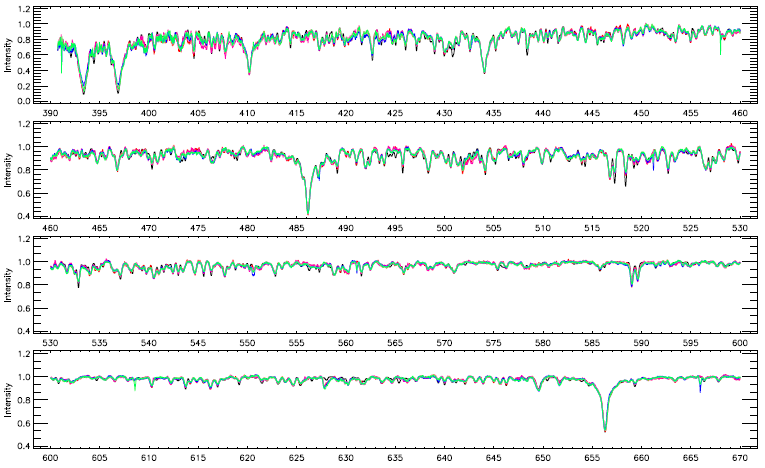
Fig. 2 Observed spectra of KOI-258 are plotted with the most compatible synthetic template derived for 6500±200 K with the metallicity of [M=H] = 0:00. In the figure, the observed spectrum is shown by thin lines in different color, while the synthetic template is shown by thick line in black. The color figure can be viewed online.
Considering the remarkable flare activity, we checked whether there is any sign of magnetic activity in the spectrum. First, we compared four spectra among themselves depending on the synthetic template for the Ca II H, K and Hα lines, as shown in upper-left panel of Figure 3. There is a clear excess and some variation in Ca II H, K, while variation is hardly visible in the case of the Hα lines seen in the bottom-left panel.
We noticed that the spectrum regions of Mg I b (λ5167Å, λ5173Å, λ5184Å) triplets and Na I D1 (λ5896Å) and D2 (λ5890Å) are clearly incompatible with the synthetic template, while all the observed spectrum parts can be fitted very well with the synthetic templates. These lines match none of the templates derived by different parameters. The Mg I b triplets and Na I D1, D2 lines are plotted with the templates in the right panel of Figure 3. In the figure, as in Figure 2, each observed spectrum part is plotted with a thin line of different color, while the synthetic template spectrum is plotted with a thick line in black. Here it must be noted that the Mg I b triplets and Na I D1 and D2 lines are well known to be sensitive to magnetic activity.

Fig. 3 Ca II H (λ3968Å), K (λ3934Å) and Hα (λ6563Å) in the observed spectra are plotted with the lines taken from the synthetic template in the left panels, while the variation of Mg I b (λ 5167Å, λ5173Å, λ5184Å) triplets, Na I D1 (λ5890Å) and D2 (λ5896Å) lines are shown in the right panels. The symbols in each panel are the same as in Figure 2. The color figure can be viewed online.
The cross-correlation functions indicated that KOI-258 is a single source as explained above. However, examining the lines shown in Figures 3 and 4, it will be easily observed that the core wavelengths of the lines have some variations. We tried to determine whether there is any radial velocity variation of KOI-258.
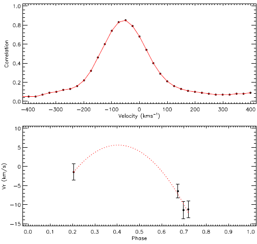
Fig. 4 A sample of the obtained cross-correlation functions and the radial velocities is plotted. In the upper panel, the cross-correlation function is shown. The observed radial velocities of KOI-258 are shown in the bottom panel. The filled circles represent observations, while the line represents the cross-correlation function, and the dotted line is a polynomial curve of second order to show one of the possible variations, as an example. The color figure can be viewed online.
To determine the radial velocity, we used the spectra of iot Psc (HD 222368, F7 V, Gray et al. 2006) as a radial velocity template. Using the FXCOR task, we cross-correlated it with each KOI-258 spectrum following the same procedure, in which the absorption lines between 5000Å and 6500Å were used (except for broad or strongly blended lines among them) for the cross-correlation function.
The cross-correlation functions indicate that the target has a single signal over the acceptable level of S/N ratio. A sample of the obtained cross-correlation functions is plotted for a phase of 0.6972 in the upper panel of Figure 4. We list measured radial velocities in Table 1, together with brief information on the observed spectra as shown in the bottom panel of Figure 4.
Table 1 Measured radial velocities*
| HJD (24 00000+) | Orbital Phase | Exposure Time (s) | Vr (kms-1) |
| 57964.36250 | 0.698 | 3600 | -11:428 ± 2:328 |
| 57964.45115 | 0.719 | 3600 | -11:238 ± 2:158 |
| 57997.51822 | 0.673 | 3600 | -6:463 ± 1:778 |
| 57995.57256 | 0.205 | 3600 | -1:461 ± 2:125 |
*Whith their standard errors and brief information on the observed spectra
3.2.The Variation at Out-of-Minima
The light variation shown in Figure 1 indicate an evident sinusoidal variation. Considering the presence of prominent flare activity clearly seen in the figure, one can think that this sinusoidal variation might be caused by a stellar cool spot. However, when the light variation is examined cycle by cycle, it is clearly observed that the shape of the light curve rapidly changes from one cycle to the next, sometimes in the same cycle. This variation cannot be caused by stellar spots. If the variation were caused by spots, the shape of the light curve would change, but not from one cycle to the next. Considering this situation and the temperature of the target, we searched the frequencies of the variation to see if it could be an effect of stellar pulsation.
We used the SC data to search for possible frequencies. First, all flares and minima were removed from the SC data. In the analysis, we used the software (Lenz & Breger 2005) that is based on the Discrete Fourier Transform (hereafter DFT) method (Scargle 1982). We faced a problem initially because the software installed on the best computer system we have could not analyse whole SC data in one step. More than a few weeks were required to find just one frequency. To solve this problem, we divided the SC data into three parts, considering the time gaps in the data as shown in the upper panel of Figure 1.
We found the frequencies with this solution: 140 frequencies were acceptable according to their 3σ levels from each data part, as shown in Figure 5, for a total of 420 frequencies; they are tabulated in Table 2. The first five lines are given in this paper, the rest are given in the online archive of the journal. In the table, the data part number is listed in the first column; the number of frequencies in that part is listed in the second column; the found frequency, the amplitude of the signal and its phase are listed in the following columns. To determine which pulsation types the target exhibits, we plot the target on the plane logT-logL in Figure 6. The frequencies found are able to model the variation seen out-of-minima. We derived the synthetic curve using equation (1) described by Scargle (1982)) and Lenz & Breger (2005) .
where A0 is the zero point, θ is the phase, Ai and Bi are the amplitude parameters. In Figure 7, we plot the residual data without any flares for each data part. In the figures, the models derived with the frequency parameters listed in Table 2 via equation (1) are also plotted with a smooth red line. As shown in the figures, the frequency parameters perfectly fit the residual data. It should be noted here that the data for the first panel are shown in this paper, while other two panels are derived for the two partial data given in the online archive of the journal.
Table 2 Frequency list of solar-like pulsation fund
| Part No | Frequency No | Frequency (d-1) | Amplitude (Intensity) | Fourier Phase |
| Part 1 | F1 | 0.9749192 ± 0.0000200 | 0.0000298 ± 0.0000002 | 0.0638716 ± 0.0009652 |
| Part 1 | F2 | 0.9651721 ± 0.0000778 | 0.0000112 ± 0.0000003 | 0.5867471 ± 0.0044517 |
| Part 1 | F3 | 0.6888211 ± 0.0000307 | 0.0000346 ± 0.0000011 | 0.0723017 ± 0.0063921 |
| Part 1 | F4 | 0.6714099 ± 0.0000247 | 0.0000242 ± 0.0000002 | 0.0909970 ± 0.0012073 |
| Part 1 | F5 | 0.9880577 ± 0.0000039 | 0.0006001 ± 0.0000011 | 0.0784607 ± 0.0003106 |

Fig. 5 The Fourier amplitude spectrum derived by using the DFT is plotted for three parts of the data.
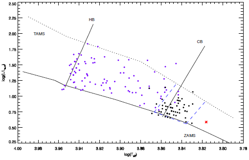
Fig. 6. Location of the target in the Hertzsprung Russell diagram. The small filled black circles represent 𝛾 Doradus type stars as listed in (Henry et al. 2005); the red asterisk represents the target. The dash dotted lines represent the borders of the area, in which γ Doradus type stars occur. Also plotted are the hot (HB) and cold (CB) borders of the δ Scuti stars for comparison. The small filled purple circles represent some semi- and un-detached binaries taken from Soydugan et al. (2006 and references therein). The ZAMS and TAMS were taken from for Z = 0.2; the borders of the instability strip were computed from Rolland et al. (2002). The color figure can be viewed online.

Fig. 7 The light variation out-of-minima are plotted for KOI-258 together with the synthetic model fit derived with Part 1's frequency parameters tabulated in Table 2. In the panels, filled circles in black represent the residual data, smooth lines represent the model fit. Similar synthetic model fits derived for the other two parts are given in the online archive of the journal. The color figure can be viewed online.
3.3.Orbital Period Variation
According to the spectral analyses, KOI-258 is not a binary star despite the existence of a radial velocity variation. However, if the averaged light curve shown in the bottom panel of Figure 1 is carefully examined, it will be noticed that a minimum in phase 0.00 appears to be the primary minimum, but also that a second one in phase 0.50 seems to be the secondary minimum. The light curve appears to be that of an eclipsing binary system. Considering the system as a binary, we checked whether there is any variation in the minima times.
First, using the frequencies described in the previous section, we removed all the sinusoidal variation from the SC data as well as all the flares. Then, all the detectable times of minima were computed without any extra correction on the residual data. Because of the dominant flare activity, we cannot detect the minima times in some data parts. Especially, we cannot detect times of the secondary minima due to low S/N ratio. After determining minima times, we computed the differences between observations and calculations, which were calculated by using the light elements given in equation (2) Slawson et al. (2011), to obtain the residuals (0-C)I .
In total, we obtained 172 minima times from the primary minima with the largest amplitude, and we grouped them in one data set (Min I). In addition, 29 minima times were obtained from the secondary minima with small amplitude; we grouped these minima in the second data set (Min II). Using the regression calculations, a linear correction was applied to the differences separately for each data set, and the (0-C)II residuals were obtained for each one. After the linear correction on (0-C)I, new ephemerides were calculated for both the primary and secondary minima as:
The first five minima times are listed in Table 3, the full table is given in the online archive of the journal. We show the variations of both (0-C)I and (0-C)II residuals in Figure 8 for the data sets of Min I and II.
Table 3 Minima times and (O - C) I and (O - C) II residuals
| Minima Time | Epoch Number | Minimum | (O-C) I | (O - C) II |
| HJD(+2400000) | (E) | Type | (day) | (days) |
| 55279.907292 | 69.0 | I | 0.020752 | 0.015164 |
| 55284.042145 | 70.0 | I | -0.001876 | -0.007427 |
| 55288.220071 | 71.0 | I | 0.018569 | 0.013055 |
| 55292.340623 | 72.0 | I | -0.018361 | -0.023836 |
| 55296.528439 | 73.0 | I | 0.011974 | 0.006536 |
3.4. Planetary Transit
To find the cause of the minima seen in the general light variation, we tried to analyse the minima in two ways. Firstly, we assumed to be an eclipsing binary; secondly, we assumed the minima to be planetary transits.
As a first step, we tried to obtain the absolute light variation caused by the components for both cases. We first removed all detected flares from the SC data. Secondly, we removed the synthetic model fits derived with equation (1) by using the frequencies listed in Table 2. We used these residual data for both cases.
In first the case, we used the PHOEBE V.0.32 software (Prša & Zwitter 2005), which employs the 2003 version of the Wilson-Devinney Code (Wilson & Devinney 1971; Wilson 1990), to analyse the light curve under the eclipsing binary assumption. We analyzed the light curves obtained from the averages of SC data, which are shown in Figure 1. The temperature of the primary component was taken as 6500 ± 200 K as found from the spectra. The temperature of the secondary component was assumed 5781 K as given by Armstrong et al. (2014). Considering the spectral type of the components, the albedos (A1 and A2) and the gravity-darkening coefficients (g1 and g1) were taken for the stars with convective envelopes (Lucy 1967; Ruciński 1969); the non-linear limb-darkening coefficients (x1 and x2) were taken from Hamme (1993). The dimensionless potentials (Ω1 and Ω2), the luminosity (L1) of the primary component, the inclination (i) of the system, the mass ratio of the system (q), and the semi-major axis (α) were taken as adjustable free parameters. We attempted to analyse the light curves in various modes, such as the detached system mode (Mod2), semi-detached system with the primary component filling its Roche-Lobe mode (Mod4), and semi-detached system with the secondary component filling its Roche-Lobe mode (Mod5). The initial tests demonstrated that an astrophysically acceptable solution was not obtainable in any mode when we consider both the obtained stellar absolute parameters and the stellar evolution models in the analysis.
For the second case we used software to analyse the minima assumed to be due to planetary transits. In these analyses, we used just the transit parts of the light variation instead of the whole light curve. According to the Data Validation Report3 for Kepler ID 11231334 presented by the Kepler Science Operations Center Pipeline at NASA Ames Research Center, KOI-258 has five candidate planets. However, we detected just three transits. It must be noted that we also detected the reported two other transits, but the amplitudes of these transits were so small that we could not obtain any statistically acceptable models for them.
Consequently, we modelled three different transits using the JKTEBOP software. We obtained the sum of the fractional radii, their ratio, (r1 + r2, r1/r2)the orbital inclination (i) and the mass ratio (q). To obtain the radii, we used the parameters of the host star. According to the spectra, the host star is a main sequence star, whose temperature is 6500 K corresponding to spectral type F6. Using the calibrations given by Cox & Pilachowski (2000), we computed the radius of the host star as 1.26 𝑅 ⊙ ; its mass was found to be 1.30
Table 4 Parameters obtained from analyses and calculations of the transits detected in the light variation of KOI-258
| Parameter | Planet 1 | Planet 2 | Planet 3 |
| Fractional Radii Sum ((r1 + r2) | 0.22917±0.00011 | 0.12442±0.00014 | 0.00074±0.00016 |
| Fractional Radii Ratio (r1/r2) | 0.01695±0.00009 | 0.00384±0.00013 | 0.00838±0.00015 |
| Orbit Inclination i(o) | 82.20±0.23 | 84.42±0.27 | 89.99±0.43 |
| Mass Ratio (q) | 0.000010±0.000005 | 0.000010±0.000007 | 0.000005±0.000007 |
| Orbital Period (day) | 4.157444±0.000018 | 4.156251±0.000414 | 2/33.20 |
| Semi Major Axis (α) (AU) | 0.026 | 0.073 | 7.983 |
| Planet Radius (R, |
2.330 | 0.528 | 1.153 |

Fig. 8. The variations of the (0-C)I and (0-C) II residuals are shown separately for the data sets of Min I and II. The filled circles in black represent the minima times determined from the primary minima; the open circles in blue represent the minima times determined from the secondary minima. The lines in red represent linear fits applied for the correction. The color figure can be viewed online.

3.5. Flare Activity and the OPEA Model
Analyzing photometric data, a method was described by Dal & Evren (2010) and Dal (2012) depending on Gershberg (1972) to determine the light variation caused just by flare activity occurring on a star. Their method is useful only for smooth light curves without flaring events. However, KOI-258 exhibits remarkable sinusoidal variation out-of-minima due to solar-like oscillation together with transits of several planets, apart from flare activity. The situation led us to improve the method to obtain the flares of KOI-258.
As we did for determining the transits, we firstly removed all the sinusoidal variations. We used the synthetic light curve of sinusoidal variation described in § 3.2. Before determining flare light curve and computing their parameters, we removed the synthetic light curve from all SC data. Secondly we removed all the minima from the light curve. Thus, we obtained a smooth light variation containing only flare variations. Considering also the standard deviation computed from the data without any flares, we determined the beginning and the end of each flare. An example of the flare light curves in magnitude and the quiescent levels derived from the synthetic light curve are shown in Figures 10. To compute the parameters of the flares, the synthetic light curve was also used as the quiescent level for each flare at the moment it occurred. In total, 51 flares were detected from the available SC data.
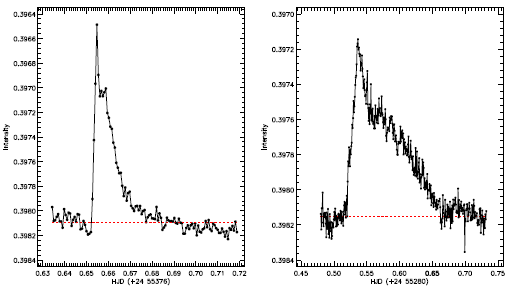
Fig. 10 A flare example detected in the observations of the system. Filled circles show observations, while the dashed line represents the level of the quiescent state of the star for the observing night. The color figure can be viewed online.
As discussed by Dal & Evren (2010, 2011), we used the flare-equivalent duration parameter in all the computations and analyses, instead of the flare energy. Considering both the beginning and the end of each flare, some flare parameters, such as flare rise times, decay times, amplitudes of flare maxima, and flare equivalent durations, were computed. The equivalent durations of the flares were computed using equation (5) taken from Gershberg (1972):
where I0 is the flux of the star in the quiet state. As described above, the synthetic light curve derived with the light curve analysis was taken as I0. However, Iflare is the intensity observed at the moment of the flare. P is the flare-equivalent duration in the observing band. All the computed parameters are listed in Table 5, whose first five lines are given in this paper, while the rest are available in the online archive of the journal. Flare maximum time, equivalent duration (P), flare rise time (Tr), flare decay time (Td), flare total time (Tt) from the beginning to the end, and flare amplitude at the moment of flare maximum are tabulated in succesive columns of the table.
Table 5 Calculated parameters of flares detected in the observations of KOI-258
| Flare Max | Equivalent Durations | Rise Time | Decay Time | Total Time | Amplitude |
| (+24 00000) | P (s) | Tr(s) | Td(s) | Tt(s) | (Intensity) |
| 55719.852734 | 0.036329 | 117.706176 | 235.394208 | 353.100384 | 0.000383 |
| 55541.086474 | 0.094022 | 176.535936 | 588.472128 | 765.008064 | 0.000370 |
| 56051.786437 | 0.201431 | 235.413216 | 588.505824 | 823.919040 | 0.000591 |
| 55469.977713 | 0.173162 | 647.325216 | 294.236064 | 941.561280 | 0.000409 |
| 55733.442779 | 0.202894 | 353.098656 | 588.500640 | 941.599296 | 0.000730 |
The distributions of equivalent durations on a logarithmic scale versus flare total durations were modelled by the One Phase Exponential Association (hereafter OPEA), using the SPSS V17.0 (Green et al. 1996) and GrahpPad Prism V5.02 (Dawson & Trapp 2004) programs.
According to Dal & Evren (2011), the OPEA function defined by equation (6) is a special function containing the Plateau term:
where y is the flare equivalent duration, x is the flare total duration as the free parameter. y0 is the flare-equivalent duration on a logarithmic scale for the least total duration. The parameter Plateau value is upper limit for the flare equivalent duration. The half-life value is half of the first x value, at which the model reaches the Plateau value. According to the definition of , the Plateau value is an indicator of the saturation level for the white-light flares. The obtained model is shown in Figure 11 together with the observed flare equivalent durations, The parameters computed from the OPEA model are tabulated in Table 6.
Table 6 The OPEA model parameters by using the least-squares method Best-fit Values
| Best-fit Values | |
| y0 | -1.46859 ±0.12025 |
| Plateau | 0.65941 ±0.12880 |
| K | 0.000332898 ±0.0000570662 |
| half-life | 2082.16 |
| Span | 2.12800 ±0.1152 |
| 95% Confidence | |
| Intervals | |
| y0 | -1.71060 to -1.22658 |
| Plateau | 0.400195 to 0.918618 |
| K | 0.000218047 to 0.000447749 |
| half-life | 1548.07 to 3178.90 |
| Span | 1.89611 to 2.35988 |
| Goodness of Fit | |
| R2 | 0.88 |
| Averaged P-value | 0.10 |
| Deviation from Model | Not Significant |
Although Dal & Evren (2011) show that the OPEA is the best function to model the equivalent duration distribution for each star, we statistically checked the model again. Using the D’Agostino-Pearson, the Shapiro-Wilk and also the Kolmogorov-Smirnov normality tests (D'Agostino & Stephens 1986), we calculated the probability value called as p-value to test whether there is any other function to fit the distribution. The p-value was found to be ≈ 0.1 and this means that there is no other function to model the distributions of flare equivalent durations (Motulsky 2007; Spanier & Oldham 1987).
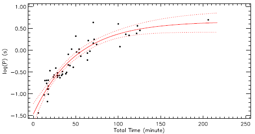
Fig. 11 The distributions of flare equivalent durations on the logarithmic scale versus flare total durations for 51 detected flares and the OPEA model derived for this distribution. Filled circles show observed flares, while the line represents the OPEA model. The color figure can be viewed online.
Gershberg (1972) described the flare frequency distribution depending on the flare energy to reveal the flare activity behavior of a star and also compared the activity levels of different stars. However, as it was described by Dal & Evren (2011), there is a problem in the comparisons of these distributions among different stars due to the stellar luminosity term in the energy computation. This is why we derived the flare frequency distribution depending on the flare equivalent duration instead of the flare energy parameter. In this study, the flare frequencies were calculated for different flare equivalent duration limits for the 51 flares. If one wants to compare the cumulative flare frequency distributions of different targets together, the cumulative flare frequency distribution must be independent of the total observing durations. Because of this, in this study, we computed the flare cumulative frequency considering the flare frequencies, which are calculated as a flare number per an hour, in each equivalent duration level. This is why the x-axis of Figure 12 has units of h-1. The obtained cumulative flare frequency distribution is shown in Figure 12. The flare cumulative frequencies exhibit a distribution in the form of an exponential function. However, in the literature, the linear part of the flare frequency distribution is generally used to compare stars among themselves. In this study, in order to determine the beginning of the linear part of the distribution, we modelled the entire distribution with an exponential function, and then we determined the turning point of the distribution, using this exponential function. The exponential function is shown by the red line in the upper panel of Figure 12. Considering the turning point, we fitted the linear part of the distribution with the correlation coefficient (R2) of 0.89 by equation (7) following the linear regression calculations:
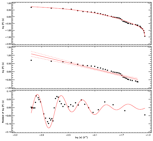
Fig 12 Cumulative flare frequencies and model calculated for KOI-258 over 51 flares are shown in the upper panel, while its liner part is shown with a linear model in the middle panel. The residuals of the model are shown in the bottom panel. The color figure can be viewed online.
In the literature, there are also two different flare frequency descriptions. described the flare frequencies, N1 as a flare number per hour and N2 as a total flare-equivalent emitting duration per hour. In the SC data taken from the Kepler Database, there are 1139.94848 day observations for KOI-258, from which 51 flares were detected. The total flare equivalent durations were found to be 50.86556 s for all these flares. We computed the frequencies described by in equations (8) and (9):
where Σnf is the total flare number, and ΣTt is the total observing duration, while ΣP is the total equivalent duration. We found that the N1 frequency is 0.00186 h-1, and the N2 frequency is 0.000052 for KOI-258.
It is well known that the flare events are generally random phenomena in the case of UV Ceti type flare stars. To test this situation for KOI-258, we calculated the phase distribution of the flares, depending on the orbital period of the target. The phase distribution is shown in Figure 13. In the figure, the distribution of the total number of flares computed in phase intervals of 0.05, for all 51 flares is shown.

4.Results and Discussion
KOI-258 is one of the controversial systems discovered in the Kepler Mission. According to some authors such as Slawson et al. (2011); Coughlin et al. (2014); Armstrong et al. (2014), KOI-258 is an eclipsing binary. They tried to estimate the physical parameters of the system. On the other hand, KOI-258 is listed as a candidate for a planetary system in several studies, such as Borucki et al. (2011); Ford et al. (2012). The target’s spectrum can give a clue. If the minima amplitudes in the light curve are considered, it can be clearly noticed that the ratio of the minima amplitudes is almost equal to 1.0. If KOI-258 were a binary system, it would be expected that the temperatures of the components be almost equal, and then, the existence of signs for the secondary component in the cross-correlation derived for KOI-258’s spectra would also be expected. However, the spectrum taken seems to be that of a single star.
Analyzing four spectra corresponding to different phases demonstrated that KOI-258 is a single star. We could not find any sign for the lines belonging to the secondary component in the cross-correlation, using the spectra of 54 Psc, HD 190404 and τ Cet with high SNR as a radial velocity templates. However, if the cores of the lines shown in Figures 3 are carefully examined, it will be easily noticed that the wavelengths of the line cores vary from one spectrum to the next. Considering this variation, we tried to determine the radial velocity of the target from each spectrum by using the spectra of the same stars as a radial velocity templates. We obtained four radial velocities corresponding to different phases, which were computed depending on the light elements given by Slawson et al. (2011). As also seen from Figure 4, there is a variation in the radial velocity of the target, and its amplitude is remarkably larger than the error bars. Considering the trend observed in Figure 4, it appears to us that KOI-258 has one or more companions, but there is no object as massive as a companion star.
Then, we tried to determine the temperature of the star by using the same comparison template stars. Because of the mismatches between the target spectra and comparison templates, we used synthetic templates to find the spectral type of KOI-258. Comparisons indicated that target spectra match the synthetic template derived for 6500±200 K with a metallicity of [M/H] = 0.00 . Thus, we decided that KOI-258 is a F6V star with solar metallicity. This result is in agreement with those given in the literature. For example, both Borucki et al. (2011) and Batalha et al. (2013) gave the temperature of the target as 6278 K with log= 4.17. However, according to Campante et al. (2014); Pinsonneault et al. (2012); Rowe et al. (2015); Huber et al. (2014), the temperature of KOI-258 is between 6528 K and 6535 K, and the log𝑔 value is between 4.161 and 4.35.
Before analyzing the whole light curve and determining the short term flares, we tried to find the cause of the sinusoidal variation at out-of-eclipses. For this aim, we considered the temperature and logg parameters determined from the KOI-258’s spectra. Then, we compared the consecutive cycles of the light curve to see whether the variation at out-of-eclipses is like that expected for stellar spot activity. We firstly considered that it is a rotational modulation effect due to cool spots, because of the presence of flare activity clearly seen in Figure 1. Examination of the light variation cycle by cycle indicated that the sinusoidal variation absolutely changes its shape in very short times, as shown in Figure 7. However, if the sinusoidal variation were caused by cool stellar spots, the frequency analysis would reveal a few dominant frequencies corresponding to the stellar period. Indeed, if the sinusoidal variation were caused by a cool stellar spot, it would be expected also that the minima phases of the sinusoidal variation should migrate, as shown for spotted stars by Yoldaş & Dal (2017b, 2019). It could be thought that the variation is caused by the stellar spots, and new spots occur in each cycle. On the other hand, it is well known that cool stellar spots can be alive for a few months. However, the active regions, where the spots occur, can be alive for several years. Therefore, if the variation were caused by the stellar spot, a regular phase migration should be observed. According to the results obtained from the spectral analyses, KOI-258 is a main sequence star of spectral type F6, which provides another possibility for this variability. The sinusoidal variation could be caused by pulsation, instead of cool spots. However, KOI-258 is located out of the instability strip in the Hertzsprung-Russell diagram. Because of this, even if KOI-258 is not a γ Doradus or δ Scuti type pulsating star, it could be a solar-like oscillating star.
Indeed, we found 420 frequencies between 0.240536±0.000014 d-1 and 6.827660±0.000003 d-1 with different amplitudes by the PERIOD04 search based on the DFT method (Scargle 1982; Lenz & Breger 2005). Using equation (1), we derived the synthetic model curve for the data with these frequencies. The concordance between observations and the synthetic curves is shown in Figure 7. According to these results, the sinusoidal variation exhibited by KOI-258 seems to be caused by solar-like oscillations. As described in § 3.2, the analyzed datasets are so large that the software cannot model the whole dataset to find frequencies. Therefore, we divided the data into three parts as shown in Figure 1. Although it appears that splitting can cause some trouble to achieve reliable results, it provides some clues to reveal the nature of the target. For instance, we did not find exactly the same frequencies from each data part, though there are a few similar frequencies found from all three parts. This indicates that the sinusoidal variation is not caused by any stable process like the rotational modulation caused by cool spots. If it were caused by a stable, semi-regular phenomenon like stellar spot activity, we would expect to find some similar frequencies and their harmonics. Therefore, KOI-258 appears to be a pulsating star. Indeed, as shown in Figure 6, the location of the target is outside the instability strip in the Hertzsprung Russell diagram. This means that the observed sinusoidal variation should be neither a γ Doradus nor a δ Scuti type pulsation. It is more likely that KOI-258 is a solar-like oscillating star, which also indicates that KOI-258 is a main sequence star, not an evolved one as mentioned by Frasca et al. (2016).
According to the spectra, KOI-258 is a single star where the minima could be caused by some orbiting planets. Despite this thought, we tried to analyse the light curve as an eclipsing binary, using the PHOEBE V.0.32 software (Prša & Zwitter 2005), which depends on the 2003 version of the Wilson-Devinney Code (Wilson & Devinney 1971; Wilson 1990). We could not reach any astrophysically acceptable solution.
There is the Data Validation Report for Kepler ID 11231334 prepared by the Kepler Science Operations Center Pipeline at NASA Ames Research Center. According to this report, KOI-258 has possibly five planets. After removing the flares and the sinusoidal variation using the derived synthetic fit, we detected several transits caused by five different planets. Two transit light curves could not be modelled due to the very low SNR, but we were able to model three of them. According to the Data Validation Report, the Planet candidates 1 and 2 have the same orbital periods of 4.2 day with the same semi-major axis of 0.1 AU. The radius of candidate Planet 1 is given as 20.2
Using the JKTEBOP software in this study, we found the sum of the fractional radii (r1 + r2), their ratio (r1/r2), the orbital inclination (i) and the mass ratio (q) as tabulated in Table 4. Depending on the temperature found from the spectra for the host star, we computed the radius of the host star as 1.26
The orbital periods of Planets 1 and 2 are so short that their transits were observed several times by the Kepler Satellite. In this case, using the orbital period given by Slawson et al. (2011) as an initial ephemeris, we adjusted their orbital periods as 4.157444±0.000018 day and 4.156251±0.000414 day for Planets 1 and 2. However, there are few observed transits for Planet 3, due to its long orbital period. Because of this, we could not adjust its period, and we used the orbital period of 233.20 day as given in the Data Validation Report for Kepler ID 11231334. In our opinion, the appearance of planet system is much more acceptable than stated in the Data Validation Report.
Apart from the sinusoidal variation and transits, the most noticeable variations observed in the light curve of KOI-258 are the instant short term flares, which are mentioned by Balona (2015) for the first time. Indeed, we found signs of magnetic activity in the spectra apart from the photometric data. For instance, the Ca II lines exhibit some excess as well as a noticeable variation, as shown in the upper panel of Figure 3. However, the Hα line reveals neither any excess nor any variation. Unexpectedly, some other lines such as Mg I b triplets and Na I D1,D2, which are indicators of the presence of magnetic instability in the stellar chromosphere, especially in the middle and upper chromosphere, exhibit both a remarkable excess and an evident variation, as seen in Figure 3.
As well as its spectra, we analyzed KOI-258’s photometric data. The target was observed by the Kepler Satellite over 1139.94848 days from HJD 24 55064.383103 to HJD 24 56204.331583, which means that the photometric data of KOI-258 cover more than 27358 hours of observing time in total. Although there are numerous data available to analyse, we could detect only 51 flares, following the method described in the § 3.5. We computed the total flare equivalent duration as 50.86556 s from 51 flares. As a result, the flare frequency N1, an averaged flare number per an hour, is 0.001864 h-1, while the flare frequency N2 is about 0.00005. In the case of the flare timescales, we found that the maximum flare total time is 4472.5 s for KOI-258, and we obtained the maximum flare rise time as 1765.46s. Moreover, the Plateau value was found to be 0.659406±0.128795 s, and the half-life is 2082.16s.
If we compare the target with the eclipsing binaries observed by the Kepler Satellite, KOI-258 has obviously a lower activity level, since the flare frequencies were found to be N1 = 0.0174 h-1 and N2 = 0.00027 for FL Lyr, N1 =0.01351 h-1 and N2= 0.00006 for KIC 9761199, N1 = 0.05087 h-1 and N2 = 0.00050 for KIC 11548140 (Yoldaş & Dal 2016, 2017b,a). The flare frequencies of are smaller than those of its analogues. The half-life is 2291.7 s for KIC 9641031, 1014 s for KIC 9761199 and 2233.6 s for KIC 11548140 (Yoldaş & Dal 2016, 2017b,a). The longest flares lasted 5178.9 s for KIC 9641031, 1118.1 s for KIC 9761199 and 22185.4 s for KIC 11548140 (Yoldaş & Dal 2016, 2017b,a). In the case of the flare timescales, has a behavior similar to the Kepler eclipsing binaries. According to the OPEA models, the Plateau values were found to be 1.232 s for KIC 9641031, 1.951 s for KIC 9761199, 2.312 s for KIC 11548140 (Yoldaş & Dal 2016, 2017b,a). Consequently, is similar to the Kepler eclipsing binaries according to the flare timescales, which means that the flares detected from KOI-258 last as long as those obtained from the Kepler eclipsing binaries. However, KOI-258’s Plateau value and the flare frequencies are smaller than in those binaries.
In the case of UV Ceti-type single stars, the N1 flare frequency was found to be N1= 1.331 h-1 for AD Leo (B - V = 1m.498), N1 = 1.056 h-1 for EV Lac (B- V = 1m.554) The N2 flare frequencies were found to be N2= 0.088 for EQ Peg (B-V=1m .574) and N2=0.086 for AD Leo (Dal & Evren 2011). Solving the OPEA models, the half-life parameters were fount to be 433.10 s for DO Cep (B-V = 1m.604), 334.30 s for EQ Peg and 226.30 s for V1005 Ori (B-V=1m.307). Moreover, the maximum flare rise times are 2062 s for V1005 Ori and 1967 s for CR Dra (B-V =1m .370) (Dal & Evren 2011), while the maximum flare total times are 5236 s for V1005 Ori and 4955 s for CR Dra (Dal & Evren 2011). According to Dal & Evren (2011), the Plateau values are 3.014 for EV Lac and 2.935 for EQ Peg, and 2.637 for V1005 Ori. If the target is compared with UV Ceti type single stars, KOI-258 has obviously a lower activity level. The observed flares have very low energies, and the target’s flare frequencies are also much lower.
In order to reveal where KOI-258 is located among similar targets regarding flare activity, we derived the cumulative flare frequency distribution depending on the flare equivalent duration instead of the flare energy. In the literature, a similar model was derived recently for KIC 12418816 (one of the most interesting systems) by Dal & Özdarcan (2018). If their flare cumulative frequency distributions are compared, it will be seen that the interval of flare cumulative frequencies is spread from log (V) of -1.50h-1 to 0.00h-1 for Group 1 and from to +0.30h-1 for Group 2 in the case of KIC 12418816, while it is spread from log (v) of -3.1h-1 to -1.3h-1 for . In addition, the log (P) values vary from -1.00 s to 2.50 s for Group 1 and from -1.00 s to 1.50 s for Group 2 of KIC 12418816; the log(P) values vary from to 0.70 s for KOI-258. Considering the variation intervals of both log (v) and log (P), it seems that KIC 12418816 is able to exhibit more frequent flares with higher energy than those KOI-258 exhibits. According to some authors such as Gershberg (1972); Gershberg & Shakhovskaia (1983); Haisch et al. (1991); Gershberg (2005), the occurrence of more frequent flares with higher energy is an indicator of high level magnetic activity as well as fast rotation due to binarity or a younger age, as estimated for KOI-258 by Walkowicz & Basri (2013).
UV Ceti type flare stars exhibit a random flare distribution in time. However, recent studies such as Yoldaş & Dal (2017b), Dal & Özdarcan (2018) and Yoldaş & Dal (2019) indicate that flares tend to aggregate around certain phases. The flare number distribution shown in Figure 13 indicates two important cases, which indicates that KOI-258’s flares occur in each phase, and occur randomly as well, as do those on UV Ceti type single stars.
According to these results, KOI-258 is a single star with three planets. The target exhibits magnetic activity, though its level is very low, which indicates that KOI-258 should be a star older than that estimated by Walkowicz & Basri (2013). If the target were a younger star, the activity level would be similar to that observed in the case of UV Ceti type stars. On the other hand, if the target were a binary system, it is expected that the activity level would be higher than it is. Finally, analyses of both photometric and spectroscopic observations reveal an interesting system. It appears that exhibits pulsation (solar-like oscillations) as well as flares. According to the spectroscopic observations, the target should be a single star hosting a planetary system consisting of three planets.

