


 nueva página del texto (beta)
 Inglés (pdf)
 Artículo en XML
 Referencias del artículo
 Enviar artículo por email
 Citado por SciELO
  Similares en
SciELO
Similares en
SciELO 
 Permalink
1.INTRODUCTION
The evolution of galaxies during cosmic time is the story of the cycle of transformation of gas into stars, the production of metals inside these stars, the release of metals during stellar life and death, and the interaction between these processes and their environment, i.e their host galaxies’ dynamics and overall structure. All this evolution leaves signatures in the observed properties of galaxies that we can analyse to reconstruct it. The analysis of this fossil record is a key tool to understand how galaxies in the nearby universe evolved. In combination with the massive acquisition of spectroscopic data, both integrated , and spatially resolved our understanding of the processes that govern galaxy evolution has increased considerably.
In a recent review, , the most recent results obtained by the analysis of Integral Field Spectroscopy (IFS) Galaxy Surveys (GS) were summarized. Among the results reviewed there were the following: (i) the sources of ionization across the optical extent of galaxies; (ii) the interplay among the global (i.e., integrated/characteristic) properties of galaxies, the local (i.e., spatially resolved) ones, and the link between these two kinds of relations; and (iii) the radial distributions of different properties of the stars and ionized gas. However, due to the narrow scope and space limitations of such reviews, some important aspects of those results were not fully addressed.
In particular, it was not possible to include a detailed description of the adopted dataset (a compilation of publicly accessible IFS data), and the description of the analysis performed to derive the results. We include those details in the current manuscript. Furthermore, we now (i) provide additional detail on the nature of the different ionizing sources and how the ionized gas is observed in galaxies; (ii) demonstrate analytically how local and global relations are connected and (iii) provide a quantitative statement on the gradients described in Sánchez (2020).
The main aim of the current article is to provide the details that were not covered in , presenting more quantitative results. Even though the two article are clearly complementary, the current one presents results not described in detail in that review and includes new ones. This review is organized as follows: (i) a description of the adopted dataset is provided in § 2; (ii) § 3 includes a summary of the performed analysis; (iii) the results of the analysis are presented in § 4, including a detailed description of the different sources of ionization within galaxies and the diagnostic diagrams widely used to disentangle them through observational signatures; (iv) the analytical description of the connection between local and global relations is included in § 5, showing that indeed both relations are essentially the same; (v) finally, a quantitative statement on the radial gradients and characteristic values of the different resolved properties explored in is included in § 6; we summarize our results and the main conclusions in § 7.
2.Data Sample
We adopted the same dataset already presented in . This represents a compilation of the publicly accessible IFS data provided by the most recent IFS-GS and compilations, including: AMUSING++ (447 Galbany et al. 2016), eCALIFA (910 Sánchez et al. 2012a; Galbany et al. 2018), MaNGA (4,655 Bundy et al. 2015b) and SAMI (Croom et al. 2012, 2,222). Details of the particular characteristics of each survey and the differences between the provided data are discussed in detail in Appendix A of Sánchez (2020). They all provide spatially resolved spectroscopic information of large samples of galaxies mostly located at z≈0.01-0.06. After removing a few cubes with low-S/N, or covering just a fraction of the optical extent of the target galaxies, the final compilation comprises 8203 galaxies, 5637 with morphological information. However, due to the strong differences among the surveys, not all galaxies are sampled with the same quality. Thus, we select what we consider the best quality data, in terms of the ability to explore the spatial variations of galaxy properties in an optimal way, by restricting the dataset to those galaxies/cubes that satisfy the following criteria:
(i) They should have a reliable morphological classification. This is extremely important since one of the main goals of the current exploration is to characterise the physical resolved properties of galaxies for different morphological types.
(ii) They should be sampled out to 2.5 effective radii ( 𝑅 𝑒 ). This requirement was included to explore only those galaxies with IFS data covering a significant fraction of their optical extension. This is particular important for disk-dominated late-type objects, whose bulge may cover a range up to 0.5-1.0 𝑅 𝑒 , (e.g. González Delgado et al. 2014) since the average properties of the disk would not be well covered if the FoV of the IFS data is limited to 1-1.5 𝑅 𝑒 . Furthermore, it is known that beyond 2 𝑅 𝑒 disk galaxies may present a different behavior than that of the main disk, showing truncations or upturns in their surface-brightness (e.g. van der Kruit 2001; Bakos et al. 2008; van der Kruit & Freeman 2011), and deviations from the global oxygen abundance trends (e.g. Marino et al. 2016). But is is also relevant in elliptical galaxies, in particular those that present some remnants of star-formation in the outskirts, but nowhere else (e.g. Gomes et al. 2016b). Thus, to cover up to 2.5 𝑅 𝑒 guarantees that we sample the real radial distributions in galaxies, not being biased to either the properties of the very central regions or those of the outermost ones.
(iii) 𝑅 𝑒 should be at least two times the full-width-at-half-maximum (FWHM) of the point spread function (PSF) of the data. This is indeed a basic requirement to guarantee that galaxies are resolved by the data. If the PSF FWHM is of the order of or larger than Re, the considered galaxy would be unresolved. Thus, even if it is sampled beyond its full optical extension no reliable gradient or variation across the FoV could or should be derived. Although this may sound obvious it is sometimes ignored, in particular since sometimes there is confusion between the size of sampling element (e.g., the pixel or spaxel in which the data are recorded or stored) and the resolution (given by the FWHM of the PSF or beam of the instrument or final dataset).
(iv) We limit the redshift range up to z < 0.02. This requirement was included to restrict ad maximum the range of cosmological distances sampled by the data (DL< 90 Mpc, 𝑡<380 Myr), but without excluding a significant fraction of galaxies of a particular type (mostly morphology) or stellar mass. This way there is no space for a strong cosmological evolution of the properties between the galaxies sampled at higher and lower redshifts, and most of the galaxies would be sampled at a similar physical resolution. Some of the original samples from which our collection is drawn span through much larger cosmological times (up to z≈0.15), with strong correlations between galaxy properties and redshift (e.g. Wake et al. 2017). This creates a complication in the exploration of the dependence of the derived observables on either the properties of the galaxies and/or their cosmological evolution.
(v) Highly inclined galaxies are excluded (i.e. we require i< 75 o ). It is known that when a galaxy is observed at high inclinations many of its global and spatial resolved properties are strongly biased . Although this is a general problem, it is obviously more evident in disk-dominated galaxies. There is a combined effect of (a) dust attenuation, that obscures more the inner than the outer regions of inclined galaxies, (b) the intrinsic differences between radial and vertical variations, and (c) the difficulty to deproject the observed properties. For instance, disk-galaxies with prominent bulges, bars or thick disks would present strong vertical variations that should not be assigned to radial differences (e.g. Levy et al. 2018). Although these galaxies are very important laboratories for the exploration of some particular and relevant galactic processes, like outflows (e.g. López-Cobá et al. 2019), they are not suitable to provide representative properties of galaxies in general (e.g. Ibarra-Medel et al. 2019).
(vi) The field-of-view (FoV) covered by the IFS data should have a diameter of at least 25´´. This requirement is introduced to have a good sampling of the radial properties of the galaxies. Considering that the PSF FWHM of the collected data range between ≈1´´ (AMUSING data), and 2.5´´ (the rest of the IFS-GS), and that we have imposed that galaxies are sampled at least up to 2.5 Re, with an Re of at least 2 times the PSF FWHM, the current requirement guarantees that we have between 5 and 10 resolution elements to explore the radial distributions. Below this number we consider that the derived gradients would not be very reliable.
This well resolved sub-sample contains almost 1,500 galaxies. In this review we sometimes adopt the full dataset, sometimes the well resolved one, depending on which is more appropriate. We clearly indicate which sample is used to derive each result.
Figure 1 shows the main properties of the compiled sample of galaxies, including the morphological distribution against stellar mass, B - R color, effective radius and the ratio between velocity and velocity dispersion (within one Re). In general the compiled sample resembles, in the observed distribution of these properties, what would be observed for a volume complete sample in a similar redshift range. For comparison purposes we have included in Figure 1, when feasible, the locus of the galaxy sample by Nair & Abraham (2010) from SDSS DR4 at a redshift range similar to ours. Our compilation is dominated by late-type galaxies (≈ 70%), with a clear peak at Sb/Sbc, and a decline towards earlier types, in particular concerning elliptical galaxies. As expected, there is an increase of the average stellar mass from late- to early-types, from

Fig. 1 Distribution of stellar masses (top-left panel), B - R color (top-right panel), effective radius (bottom-left panel) and v /σ ratio within one effective radius (bottom-right panel) versus the morphological type for the full sample of galaxies. Symbols have the same meaning in each panel. Boxes are located at the average value for each morphology bin, with the size in the y-axis corresponding to the standard deviation around this value. Colors represent the mean value of the EW(Hα) of the galaxies, and error bars indicate the range of values covered by 98% of the sample, in each bin and for each of the explored parameters. In addition, for the first three panels, we include, as grey-dashed contours, the density distribution reported by Nair & Abraham (2010) for a sub-sample of the galaxies in the SDSS survey, located at a similar redshift range. The color figure can be viewed online.
However, despite these differences, the overall trend between morphology and stellar mass is very similar. Both in Sánchez (2020) and the current exploration we try to separate the effects of stellar mass and morphology dividing galaxies in mass/morphology bins. However, it is worth noticing that in this type of segregation there are intrinsic biases. In particular, groups of early-type galaxies (E/S0) and low stellar mass (
A trend similar to the one observed between morphology and mass is observed between B - R color and mass (e.g. Balogh et al. 2004). Early-type galaxies are red, covering a very narrow range of colors (i.e., defining a clear red sequence at B-R ≈ 1.2 mag). Later-type galaxies have bluer colors, covering a wider range of colors (i.e., a cloud rather than a sequence). The most relevant difference between the two groups is that there is a deficit of blue/early-type galaxies (E/S0, B- R < 0.5 mag) and a corresponding deficit of red/late-type galaxies (Sc/Sd, B- R > 0.8 mag). Again, this distribution resembles what would be observed in a volume limited sample at a similar cosmological distance.
Regarding the sizes of the galaxies, characterized by the effective radius ( 𝑅 𝑒 ), there is also a relation with morphology. However, this seems to be a secondary correlation arising because of the well known relation of Re with stellar mass (e.g. Conselice 2006, 2012; Sánchez 2020, Figure 20). However, this trend is more shallow than the one with M*. On average, early-type galaxies are slightly larger and cover a wider size range than late-type galaxis. This trend has a large dispersion and, for a given morphology, galaxies present a wide range of sizes, although in general there is a lack of spiral galaxies larger than Re > 10 kpc (for galaxies later than Sb). This figure shows that size is primarily dependent on galaxy mass, rather than morphology. When comparing with the literature results, there are clear differences. The data of Nair & Abraham (2010) show a sharper increase in size from Scd to Sab galaxies, with a drop for earlier type galaxies. This distribution is not expected naively, and could be related to a size bias in that sample rather than a real effect. In any case, the average values are not very different between the two samples.
Finally, we present the distribution of the ratio between stellar rotation velocity and velocity dispersion within one Re over morphology. This ratio is a proxy for the fraction of ordered rotation in these galaxies . Large values correspond to galaxies with stars following well ordered orbits distributed in a plane or disk, i.e., cold, rotationally supported orbits. On the contrary, low values correspond to galaxies with stars on hot/warm orbits (pressure supported), with a triaxial structure, including galaxies with strong bulges . As expected, early-type galaxies present the lowest values for the v/𝜎 ratio, with a mode ≈0.1 and a deficit of galaxies with v/σ >0.5 for pure ellipticals. On the other hand, late-type galaxies present the largest values, with a mode ≈ 0.5 (for Sc/Sd) galaxies. It is interesting to highlight that the range of values covered by this parameter for late-type galaxies is also wider, which is a consequence of projection effects. Like in the case of the previous figures, the observed distribution for the compiled sample agrees with the expected one for galaxies in the nearby Universe . (e.g. Davies et al. 1983)
The symbols in the panels of Figure 1 are color-coded by the average distribution of the equivalent width (EW) of the H𝛼 emission line. As extensively discussed in different studies (e.g. Stasińska et al. 2008; Cid Fernandes et al. 2010; Sánchez et al. 2018) and reviewed in Sánchez (2020), this parameter segregates well between star-forming and retired galaxies (SFGs/RGs). It separates equally well between star-forming and retired areas (SFAs/RAs) within galaxies . The distributions shown in Figure 1 illustrate clearly the connection between the different global properties and the star-formation activity of galaxies. Early-type, massive, red, large and pressure supported galaxies are mostly RGs, with little or no star-formation. On the contrary, late-type, less massive, bluer, smaller and rotationally supported galaxies are mostly SFGs. Thus, those are the galaxies that contribute most to the star formation budget in the nearby universe. There are clear, continuous trends from SFGs to RGs, just as from late to early type galaxies, with most galaxies in the transition region between the two groups corresponding to early spirals (Sa/Sb), i.e. spirals with prominent bulges.
In summary, the compiled sample of galaxies covers the space of explored parameters just as well as a well-defined, statistically significant sample at the same cosmological distance. In general, the distributions are similar to those reported for this kind of samples (e.g. Blanton & Moustakas 2009). Therefore, although our sample was assembled in an ill-defined manner, the properties and results extracted from its analysis can be considered a good representation of the average population of galaxies in the nearby Universe (i.e. within a few hundred Mpc).
3.Analysis
To provide a homogeneous analysis of this somewhat heterogeneous dataset we analysed all cubes using the same tool, the Pipe3D pipeline . This pipeline was designed for IFS datacubes to (i) fit the stellar continuum with spectra from stellar population models and (ii) extract the information about the emission lines of ionized gas. Pipe3D uses FIT3D algorithms as basic fitting routines (Sánchez et al. 2016b) 1. We include here a brief description of the fitting procedure (extensively described in Sánchez et al. 2016b,a), and a more detailed description of how the different parameters used in this review (and in Sánchez 2020) were derived.
3.1.Stellar Population Analysis
The fitting of the stellar continuum requires a minimum signal-to-noise ratio (S/N) to provide reliable results. Since it is not guaranteed that this S/N is reached throughout the entire FoV (or optical extent of the galaxy), as a first step, a spatial binning is performed in each datacube to increase the S/N above this limit by co-adding adjacent spectra. This limit was selected to be 50 for most of the compiled data (CALIFA, MaNGA and AMUSING++), and 20 for the SAMI data (which have slightly lower S/N in the continuum). The actual value of this S/N limit was derived based on simulations for the spectral resolutions and wavelength ranges covered by the data (Sánchez et al. 2016b).
Then, the stellar continuum of the co-added spectra corresponding to each spatial bin was fitted with a stellar population model, taking into account a model for the line-of-sight velocity distribution (LOSVD), and the dust attenuation. The stellar population model consists of a linear combination of a set of simple stellar populations (SSP) taken from a particular library. Therefore, the model spectrum is described by the following equation:
where Sobs(λ) is the observed intensity of the spectrum at the wavelength 𝜆 for a particular bin; Smod(λ) is the overall model, which is derived by minimizing the difference with respect to Sobs(λ) (by means of x2 minimization); wssp is the normalization of each contributing model SSP spectrum Sssp(λ); AV is the dust attenuation in the (in magnitudes), and E(λ) is the adopted extinction curve Cardelli et al. 1989). This unbroadened model spectrum is convolved with the LOSVD, G(v, σ), modelled by a Gaussian function of two parameters (the velocity, 𝑣, and velocity dispersion, σ). Thus, the best fitting model comprises three non-linear parameters (AV, v and σ), and a set of linear parameters, wssp, one for each SSP in the considered library. Note that equation 1 assumes that the kinematics of all stars is described with a single LOSVD, and that they are all affected by a single dust attenuation. These are simplifications of the problem. Young and old stars are known to follow different orbits within galaxies, and they may be affected by different dust attenuation. Experiments with more complex decomposition procedures are described in Vale Asari et al. (2016).
Each SSP in the library is represented by a single spectrum, which is the result of co-adding all the spectra of the surviving stars (i.e., considering the mass-loss with time, e.g. Courteau et al. 2014) created by a single burst that happened a certain time in the past (i.e. the age of the SSP) from gas with a certain chemical composition (i.e. a certain metallicity). SSPs are created by stellar population synthesis codes (e.g. Bruzual & Charlot 2003), using as basic ingredients: (i) an initial mass function (IMF) of stars (e.g. Salpeter 1955; Chabrier 2003); (ii) a model for the evolution of the stars, described by isochrones in the Hertzsprung-Russell diagram; and (iii) a synthetic (e.g. Coelho et al. 2007; Maraston et al. 2010) or observational (Sánchez-Blázquez et al. 2006) stellar library of spectra for each star with a particular set of physical parameters (i.e. at each location within the HR diagram and for each metallicity). The different ingredients included in the generation of the SSP, and differences in the model algorithms, produce subtle differences in the synthetic stellar population spectra for the same physical parameters. Therefore, any inversion method/stellar decomposition like the one described before (equation 1) may produce different quantitative results depending on the adopted SSP library. The limitations of this method have been described in more detail elsewhere (Walcher et al. 2011; Conroy 2013).
The adopted implementation of Pipe3D uses the GSD156 SSP-library. This library, first described in Cid Fernandes et al. (2013), comprises 156 SSP templates, that sample 39 ages (1 Myr to 14 Gyr, on an almost logarithmic scale), and 4 different metallicities (
We should stress that this particular library is not a priori better than others adopted to derive the properties of the stellar populations. Detailed comparisons and simulations presented in different studies (e.g. Cid Fernandes et al. 2014; González Delgado et al. 2014; Sánchez et al. 2016b,a; González Delgado et al. 2016), demonstrate that, as long as the space of parameters is fairly covered (mostly expected ages and metallicities), the explored quantities are well recovered and/or the values are consistent at least qualitatively when using different SSP templates. The main reason why the GSD156 library is best placed for the current study is because it is the only one used to explore in common the different datasets comprised in this study and, at the same time, has been confronted against mock IFS observations of galaxies created from hydrodynamical simulations . Therefore we understand better the systematics associated with the derivation of parameters than with other SSP templates.
Once the best model for the stellar population in each bin was derived, the model was adapted for each spaxel. This was done by re-scaling the model spectrum in each bin to the continuum flux intensity at the considered spaxel, as described in and (we say that the model is “dezonified”). Finally, based on the results of the fitting, it is possible to derive different physical quantities in each parameter P, both light-weighted (LW) and mass-weighted (MW), using the formulae:
and
where: (i) P is the considered parameter, (ii) wssp are the light weights
(normalizations) described in equation 1, and (iii) M/L
ssp
is the mass-to-light ratio of the SSP. The parameters can be derived both
in a spatially resolved way (spaxel-by-spaxel or bin-by-bin) or integrated (on
coadded spectra or averaged across the FoV). These equations are also used in
Sánchez (2020) and the current
review to obtain further quantities of interest. Among them the most relevant
are: (i) the average light-weighted mass-to-light ratio (M/L) , obtained by
substituting P by M/L
ssp
in equation 2; (ii) the stellar mass surface density (
where DL is the luminosity distance and Aspax is the area of each spaxel (in the corresponding units, pc2 in the present review). By integration over the FoV it is possible to derive the integrated stellar Mass (M*); (iii) in a similar way, if instead of co-adding all the ages included in the SSP library, both quantities are added from the beginning of star formation in the universe up to a certain look-back time (and with additional corrections for the mass-loss), it is possible to derive M*,t and
where t1 and t0 are two look-back times (where t1 < t0 and t0 - t1 is relatively small). This way it is possible to estimate the most recent SFR from the stellar population analysis, usually defined as SFRssp =SFR32Myr (González Delgado et al. 2016) (although other time ranges, in general below 100 Myr, are considered too)3; (v) the LW and MW Age (
3.2.Analysis of the Ionized Gas
In conjunction with the analysis of the stellar population we explore the properties of the ionized gas (both resolved and integrated) by deriving a set of emission line parameters, including the flux intensity, equivalent width and kinematic properties. To that end, we create a cube that contains just the information from these emission lines by subtracting the best fitting stellar population model, spaxel-by-spaxel, from the original cube. This gas-pure cube inherits a variance vector from the original cube which is made from two components: the original noise associated with the observations and the standard deviation of the residuals obtained from a Monte Carlo run of the continuum fitting with stellar population models. Finally, the parameters for each individual emission line within each spectrum at each spaxel of this cube are extracted using a weighted momentum analysis as described in Sánchez et al. (2016a). More than 50 emission lines are included in the analysis in the case of the CALIFA, MaNGA and SAMI datasets, and around 20 lines in the case of MUSE. Among them we include the strongest emission lines within the optical wavelength range: Hα, Hβ, [OII] 𝜆37274, [OIII] 𝜆4959, [OIII] 𝜆5007, [NII] 𝜆6548, [NII] 𝜆6583, [SII]𝜆6717 and [SII]𝜆6731. The final product of this analysis is a set of maps showing the spatial distributions of the emission line flux intensities and equivalent widths. Integrated (or averaged) quantities across the optical extent of galaxies (or across the FoV of the instrument) are then easily derived.
Finally, as in the case of the stellar mass, we derive the spatial distribution of different physical quantities used in the present review (and throughout Sánchez 2020): (i) The attenuation of ionized gas emission ( 𝐴 𝑉 ), derived from the spatial distribution of the Hα/Hβ ratio. We adopt the canonical value of 2.86 (Osterbrock 1989) for the non-attenuated ratio and use a Milky Way-like extinction law (Cardelli et al. 1989) with Rv=3.1. (ii) The SFR, both resolved (i.e. the SFR surface density,
Based on these primary parameters, we can also derive some additional parameters discussed within this review: (i) Star-formation efficiency, defined as the ratio between the SFR and Mgas (or between
All the physical parameters derived from emission lines are not directly calculated by Pipe3D, although they are part of a post-processing analysis that is performed by the same algorithms for the different datasets. Finally, we should strongly stress that Pipe3D is just one of several different pipelines/tools developed in the last years with the goal of analysing IFS data (e.g., PyCASSO, LZIFU, MaNGA DAP de Amorim et al. 2017; Ho et al. 2016; Belfiore et al. 2019). Most of the performed comparisons demonstrate a remarkable agreement in the results (Sánchez et al. 2016a; Belfiore et al. 2019; Sánchez et al. 2019b).
4.Ionizing Sources in Galaxies
Star forming galaxies (SFGs) and star forming areas within galaxies (SFAs) are frequently identified based on the observational properties of the ionized gas. In our current understanding of the star-formation process when a molecular gas cloud reaches the conditions of the Jeans instability (Jeans 1902; Bonnor 1957) it fragments and collapses, eventually igniting star formation activity (Low & Lynden-Bell 1976; Truelove et al. 1997). This process creates thousands of stars at the typical scale of a molecular cloud, in general. These stars are not equally distributed in mass: as expected from a fragmented cloud (Bate & Bonnell 2005), there is a larger number of less massive stars than of more massive ones (Salpeter 1955; Chabrier 2003). These massive, short-lived, young stars (classified spectroscopically as O and B stars) have a blue spectrum, with a significant contribution of photons below the limit required to ionize not only hydrogen (E >13.6 eV, λ < 912Å), but also other, heavier elements, in particular oxygen, nitrogen and sulfur. Therefore, they ionize the gas distributed around the recently formed stellar cluster, producing a large number of emission lines observed in the optical spectrum. These emission lines arise due to the recombination of ions with electrons, and the subsequent cascade of lines as the electron drops onto low energy levels, or by the radiative de-excitation of electrons on levels previously excited by collisions between ions and electrons (e.g. Osterbrock 1989). These ionized gas clouds are the classical HII regions (e.g. Sharpless 1959; Peimbert 1967).
The ratios between emission lines originating from ionized metals and those from hydrogen depend on the physical conditions inside the nebulae. In general, classical regions show typical values for certain line ratios (like [OII]/Hβ, [OIII]/Hβ, [OI]/Hα, [NII]Hα and [SII]/Hα): (i) <1 dex in the case of [OIII]/Hb; (ii) < - 0.1 dex, in the case of [NII]/Hb and [SII]/Hα; and (iii) < −1 dex, in the case of [OI]/Ha . The reason for these relatively low values is the shape of the ionizing spectra, that, although hard enough to cause some ionization, are not hard enough to provide enough high energy photons to strongly ionize heavy elements like oxygen or nitrogen. These ratios are then further modulated by the oxygen and nitrogen abundances, the ionization parameter (the ratio between the available ionizing photons and the hydrogen content), the electron density, dust content and even the geometry of the nebulae with respect to the ionizing source (e.g. Baldwin et al. 1981a; Evans & Dopita Dopita 1985; Dopita & Evans 1986; Veilleux & Osterbrock1987; Veilleux et al. 1995; Dopita et al. 2000; Kewley et al. 2001; Kewley & Dopita 2002; Sánchez et al. 2015; Morisset et al. 2016).
However, young stars resulting from recent SF are not the only ionizing sources in galaxies (although they are in general the dominant one). Other sources, in order of importance (strength and frequency) are: (i) The hard and intense ionizing spectra associated with non-thermal and thermal emission of active galactic nuclei, which are observed in a limited fraction of galaxies. This ionization is particularly important in the central regions of galaxies, and for those galaxies in the AGN phase (≈10% of galaxies in the nearby Universe, or even less, e.g. Schawinski et al. 2010; Lacerda et al. 2020, although their relative importance increases at high-z). (ii) The hard but weak ionizing radiation from hot evolved stars (HOLMES, post-AGB stars Binette et al. 1994; Flores- Fajardo et al. 2011), that could significantly contribute to the excitation of the so-called diffuse ionized gas in galaxies (DIG, e.g. Singh et al. 2013a; Lacerda et al. 2018). (iii) Shocks associated with galactic winds, either induced by high-velocity galactic-scale winds due to the kinetic energy introduced by central starbursts (e.g. Heckman et al. 1990) or AGN, or low-velocity winds associated with gas cooling processes or internal movements in triaxial galaxies (Dopita et al. 1996). This ionization may also contribute significantly to the DIG. (iv) Supernova remnants, associated with past (but relatively recent, <100 Myr) SF processes, also present an expanding shock wave, but with very different geometry than the previous ones. Similar in shape to HII regions, and frequently misclassified or mixed with them, they could explain a fraction of the nitrogen enhanced regions described in the literature (Ho et al. 1997; Sánchez et al. 2012b, Cid Fernandes et al., submitted). In general, all those ionizing sources have harder ionizing spectra than the ones observed in regions. Therefore, they emit a relatively larger fraction of their flux in high energy photons and thus produce larger values for the line ratios described above.
When using emission lines as diagnostics of the ionized ISM, it is important to keep in mind a second concept, which we will call the “ionization conditions” in the remainder of this review. Indeed, it is customary to subsume all gas that does not reside in a spatial region clearly associated with star formation (i.e.HII regions) or clearly associated with AGN (narrow line regions NLR) into the diffuse ionized gas (DIG). The DIG is, in general, all emission that has no clear peaky structure, but has a rather smooth surface brightness distribution. DIG may still show structure (filaments, spiral arms), but to a lesser degree than is typical for HII regions.
A clear-cut case where the ionization source has to be distinguished from the ionization conditions is the leaking of ionizing photons from regions. Indeed, these photons may show a somewhat harder ionizing spectrum than the original source (hot, massive stars e.g. Weilbacher et al. 2018), and therefore show a much wider range of line ratios than the regions directly associated with the ionizing source. As we will see later, in galaxies that are primarily ionized by SF, leaked photons can contribute significantly to the DIG.
The physical differences between the possible ionizing sources listed before (mostly the hardness of their spectra), and the ionized gas (mostly their metal content) have been used to define demarcation lines in diagrams comparing pairs of metallic to hydrogen line ratios, with the intent of distinguishing between ionizing sources directly. These are the so-called diagnostic diagrams (e.g. Baldwin et al. 1981a; Osterbrock 1989; Veilleux et al. 2001). This concept is quite successful to identify gas ionized by star forming regions, which shows a nearly one-to-one correspondence between the location of the spatial regions within the diagnostic diagrams and the ionizing source (e.g. Kewley et al. 2001). Unfortunately, the distinction among the different physical processes in the second group is less clear (e.g. Cid Fernandes et al. 2010). Some of the complication arises because of the mixing between different ionizing sources. This is particularly important for those ionizing sources that contribute to the DIG, where shocks, the contribution of ionization by old stars, and even photons leaked from regions could be spatially co-existing (e.g. Della Bruna et al. 2020). We will try to shed some light on this complex problem in the next section.
4.1Complexity and Myths of Diagnostic Diagrams
Figure 2 shows the distribution of galaxies in three of the most frequently adopted diagnostic diagrams (Veilleux et al. 1995). The left panels show the distributions for the central regions of galaxies, corresponding to ≈ 1 kpc at the average redshift of our compilation (3´´ v 3´´ aperture). This region corresponds to the one most affected by any ionization associated with an AGN, a shock induced by a central outflow, or ionization due to hot evolved stars (more frequently present in the bulge of galaxies, the socalled cLIERs, e.g. Belfiore et al. 2017a). The right panels present similar distributions for a ring at one effective radius of each galaxy. This region is far enough from the center to be clearly less affected by central ionizing sources, and therefore the ionization is more related to HII regions in the case of SFGs. In all these plots each galaxy contributes as a single point in the considered distributions. The distributions are color-coded by the average value of EW(Hα) for all the galaxies at a particular locus within the diagram. As indicated before, several studies have demonstrated that the EW(Hα), in combination with the described line ratios, is a good discriminator between ionization conditions: (i) AGN and high-velocity shocks show in general high values of the EW(Hα), > 6Å. (ii) HOLMES/post-AGBs and low-velocity shocks show in general low values of the EW(Hα), < 3Å (e.g. Binette et al. 1994; Sarzi et al. 2010; Lacerda et al. 2018; López-Cobá et al. 2020). (iii) Weak AGN could show EW values between 3-6Å (e.g. Cid Fernandes et al. 2010), and sometimes even lower (for very weak ones). It is important to note here that regions are expected to show a high value of the EW(Hα) too. In our sample they show values larger than 6Å (e.g., Sánchez et al. 2014; Lacerda et al. 2018; Espinosa-Ponce et al. 2020). However, they are located in a different region in the diagnostic diagrams, as indicated before.
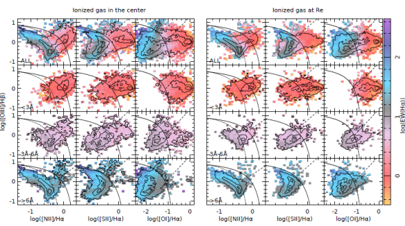
Fig. 2 Left panels: Diagnostic diagrams for ionized gas built from the central (≈ 3´´ diameter) apertures of the galaxies in the sample, including the distributions of the [OIII/Hα] vs. [NII]/Hα line ratio (left panel), [OIII/Hβ] vs. [SII]/Hα (central panel), and [OIII/Hβ] vs. [OI]/Hα (right panel). Each galaxy contributes a single point in the distributions, which in turn are shown as contours representing the density of objects. Each contour encompasses 95%, 50% and 10% of the points, respectively. The color code shows the average EW(Hα), on a logarithmic scale, of all galaxies at each point in the diagrams. In all panels the solid line represents the locus of the Kewley et al. (2001) boundary lines, with the proposed separation between Seyferts and LINERs indicated with a dashed-line. Finally, in the left-most diagram the dotted-line represents the locus of the Kauffmann et al. (2003) demarcation line. The upper panels show the distributions for all galaxies, irrespective of their EW(Hα) values. Then, from top to bottom, galaxies are separated by EW(Hα), comprising low values (<3Å, panels in the 2nd row), intermediate values ( 3-6Å, panels in the 3rd row), and high values (>6Å, bottompanels). Right panels: Similar plots for the average ionized gas at the effective radius in each galaxy. The color figure can be viewed online.
The described trends can also be seen in the average distributions shown in the top panels of both right and left figures. Ionized regions with high EW are mostly located in the left part of the diagrams, i.e., at the classical location of HII regions. On the other hand, ionized regions with low EW are found in the right parts of the three diagrams. We will show in upcoming sections that indeed low EW is in general associated with DIG. Such regions are more numerous in the left panels (central regions of galaxies) than at one Re.
There are a few galaxies with high EW regions in the upper right area of the diagram. They are clearly less numerous than the low EW ones and therefore do not show up well in our representation. Their influence can, however, be seen in the three diagrams in the last row on the left. A comparison with the three panels on the right in the same row also shows that they are more numerous in the center than at one Re. Those correspond to either strong AGN ionization or the contribution of shocks created by high velocity galactic outflows (e.g. Bland-Hawthorn 1995; Veilleux et al. 2001; Ho et al. 2014; López-Cobá et al. 2019, 2020).
As mentioned before, based on the described average distributions, different demarcation lines have been proposed in these diagrams to separate between the different ionizing sources. The most popular ones are the Kauffmann et al. (2003) (K03) and (K01) curves (included in Figure 2 as a dashed and a solid line). They are usually invoked to distinguish between star-forming regions (below the K03 curve) and AGN (above the K01 curve). The location between both curves is generally assigned to a mixture of different sources of ionization, being refereed to as the composite region (e.g. Cid Fernandes et al. 2010; Davies et al. 2016). However, as we will discuss later, this is only one of multiple possibilities to populate that area of the diagnostic diagrams. The demarcations lines have a very different origin. The K03 line is a purely empirical boundary traced by hand as an envelope of the star-forming galaxies detected in the SDSS spectroscopic survey. The second demarcation line was derived based on a set of photo-ionization models, as the envelope of the largest values for the considered line ratios that can be produced by ionization due to young stars and a continuous star formation (similar curves were derived by Dopita et al. 2000; Stasińska et al. 2006, using other photoionization models and star-formation histories). In essence, only these latter demarcation lines are physically driven, indicating which region of the diagrams cannot be populated by ionization due to star-formation.
A first exploration of the distributions shown in Figure 2 seems to demonstrate that the proposed demarcation lines do a good job of segregating at least the harder (AGN, shocks, post-AGBs) from the softer (HII) ionization. When exploring the upper panels in both figures it seems that all HII regions (high-EW, left-size) are well constrained by the K03 demarcation line, while most of the hard ionized regions are above the K01 one. This seems to be particularly true for AGN, which correspond to the hard ionized regions (upper right in each diagram) in the bottom panels (i.e., with high EWs).
However, while it is certainly true that low spatial resolution or single aperture data may mix different spatial components of galaxies with different ionization mechanisms, and thus may populate the region between the two demarcation lines, it is not true that only mixed ionization can be found there. A detailed inspection of the distributions segregated by the EW(Hα) clearly demonstrates so. High EW regions with mixed ionization could only result from the mixing of and AGN/shock ionization. However, such a case could be present only in a very limited fraction of galaxies (<10% or so, at the considered redshift), and only in the central regions of galaxies (left panels). So, in general, mixed ionization resulting from a mixture of SF and DIG should be identifiable by intermediate EW values. This corresponds to the third row of panels in both figures. While a substantial fraction of spatial regions with intermediate EW are located in the intermediate region, a considerable fraction of these are well below and above the K03 and K01 curves. Thus, there are no features in the EW-augmented diagnostic diagrams that would allow to define a unique locus of mixed ionization.
Furthermore, exploring the diagrams corresponding to the high and low EWs (2nd and 4th rows), the complete continuity in the distributions over the K01 and K03 lines seems to indicate that this intermediate region is populated by a non-negligible fraction of both DIG and/or regions . Thus, the region between both demarcations lines is not exclusively populated by spatial regions with a mixed ionization. Finally, an additional complication are the low EW regions well below both the K01 and the K03 demarcation line (in particular at one Re and for K01). Some authors have even claimed that low-metallicity AGNs could also populate a region below the K01 (or the K03) line (e.g. Stasińska 2017). This indeed does not contradict the nature of the K01 line, that was defined as a maximum envelope for the /SF regions (which seems to be a valid interpretation), and not as a definitive boundary between soft and hard ionization (as frequently and wrongly interpreted).
In summary: (i) classifying the ionizing source based only on the distribution in the so-called diagnostic diagrams may be valid only in a statistical sense. Thus, for individual targets in boundary/intermediate regions, the use of these diagrams may lead to important mistakes; (ii) considering the additional information provided by the EW(H𝛼) may mitigate the mis-classifications induced by a selection based only on the loci within these diagrams; and (iii) interpreting the location in a diagram as a combination of mixing of ionizing sources may be largely misleading. However, as we will see in the next section, additional information provided by the morphology/shape of the ionized structures, the underlying stellar population, and even the kinematics of the gas may shed some further light on the ionization conditions.
4.2.Spatial Distribution of the Ionized Gas
In this section we explore the spatial distribution of the ionized gas and the line ratios in some prototype galaxies included in our galaxy sample. The main aim of this section is to reinforce the results highlighted in the previous section, and to demonstrate how the shape/morphology and general spatial distribution of the ionized gas may help to disentangle different ionizing sources, beyond the use of just diagnostic diagrams (and EWs). We adopted only data taken with the best spatial resolution (MUSE data), although similar conclusions could be extracted from other datasets (strongly affected by resolution effects, in some cases). Figures 3, 4 and 5 show, for each of the considered galaxies, in the top-left panel, a true color continuum image. This image is reconstructed from the datacubes by convolving the individual spectra at each spaxel with the response curve of the g, r and i-band filters. Then, the three images are combined into one, with each filter corresponding to the blue, green and red color respectively. In addition, the figure shows, in the top-middle panel, a color image created using the [OIII] (blue), H𝛼 (green) and [NII] (red) emission line maps extracted from the gas-pure datacube, as described in § 3.2. These two images (continuum and emission line) allow us to explore the distribution of the ionized gas structures across the optical extent of galaxies, and its association with the different morphological sub-structures (such as bulges, disks, arms, bars..). In addition to these two maps we show, for each galaxy, four different diagnostic diagrams, including the ones shown in Figure 2, and the WHAM diagram, that compares the [NII] ratio with the EW(Hα). Thus, this figure takes into account the main conclusion of § 4.1 on the classification of the ionizing sources, mitigating the segregation problems by considering the EW(Hα) in addition to the classical diagnostic diagrams.

Fig. 3 Each panel shows, for different galaxies: (a) the continuum image created using g (blue),r (green) and i-band (red) images extracted from a MUSE datacube, by convolving the individual spectrum in each spaxel with the corresponding filter response curve (left-panel); (b) the emission line image created using the [OIII] (blue), Hα (green) and [NII] (red) emission line maps extracted from the same datacube using the Pipe3D pipeline (central-panel); (c) the WHAN diagnostic diagram presented by Cid Fernandes et al. (2010), showing the distribution of EW(Hα) versus the [NII]/Hα line ration; and finally, (d) the classical diagnostic diagrams involving the [OIII]/Hβ line ratios vs. [NII]/Hα (left), [SII]/Hα (middle) and [OI]/Hα (right), respectively (Baldwin et al. 1981b; Veilleux et al. 1995). The four diagnostic diagrams included in panels (c) and (d) are color-coded by the values shown in the emission line image shown in panel (b). The average value of the parameters shown in panels (c) and (d) across the entire FoV of the IFU data is shown as a red star in each diagnostic diagram, while the central value is marked with a blue star. The solid and dashed lines represent the location of the Kewley et al. (2001) and Kauffmann et al. (2003) demarcation lines, respectively. The name of each galaxy shown in each panel is included in the figures, comprising from top to bottom MCG-01-04-025, UGC1395, ESO0298-28 and IC1657. The color figure can be viewed online.
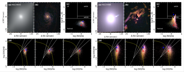
Fig. 4 Similar figure as Figure 3, for galaxies NGC4643 and NGC4486. The color figure can be viewed online.
Each pixel shown in the top-middle image is mapped with the same color in the four diagnostic diagrams, clearly showing the association between the loci in those diagrams and the spatial distribution of the ionized gas. Figure 3 shows four examples of galaxies with a considerable number of HII regions, which dominate the ionization across the galaxy disk. They are seen as clumpy/peaked ionized structures, almost circular, at the spatial resolution of these data (≈ 0.1-0.5 kpc), as described by Sánchez-Menguiano et al. (2018). They are clearly distinguished in the emission-line maps, tracing the spiral arm structure. Furthermore, they are mostly located in the lower-left region of the diagnostic diagrams, forming an arc where the classical HII regions are found (e.g. Osterbrock 1989). They are easily identified in the four considered galaxies (MCG-01-04-025, UGC1395, ESO0298-28, and IC1657).
In the case of MCG-01-04-025 all the ionization seems to be produced directly by regions (clumpy structures), with a possible component of DIG (not clumpy, smooth distribution). In this galaxy DIG is most probably due to photon leaking from those regions, being the most frequent or dominant ionizing source for the diffuse gas in late-type spirals as reported in the literature (e.g. Zurita et al. 2000; Relaño et al. 2012). The color change in the ionized gas map for the regions from the center (more green) to the outer parts (blueish), reflects both the well known negative abundance gradient in these galaxies (e.g. Searle 1971; Vila-Costas & Edmunds 1992; Sánchez et al. 2014; Sánchez-Menguiano et al. 2018), and most probably a positive gradient in the ionization parameter (e.g. Sánchez et al. 2012b, 2015).
The other three galaxies show additional ionizing conditions in their central regions. In the case of UGC1395, the almost point-like, strong and hard ionization, at the very center of the galaxy is a clear indication of the presence of an AGN. Indeed, the line ratios in this central region are located well above the K01 curve, with an EW(Hα) that in most of the cases is well above the 6Å cut proposed by for strong AGN. Despite the clear presence of an AGN, we should notice that a strict cut in the EW is not fully valid for these resolved spectroscopic data. At the edge of the distribution dominated by the AGN the EW drops below 6Å and even 3Å, just because the PSF size and/or the strong radial decline expected for this kind of ionization (Singh et al. 2013b; Papaderos et al. 2013). Thus, the inclusion of the EW(H𝛼) helps to discriminate the nature of the ionization, but without spatial information it may provide an incomplete picture.
In the central region of the next example, ESO0298-28, a hard ionization is clearly present as well. However, contrary to the previous case, although the line ratios are very similar, both the EW(Hα) (clearly below the 3Å cut proposed by Cid Fernandes et al. 2010, for retired galaxies) and the spatial distribution (smoother, following the stellar light distribution), indicate that the ionized gas has a completely different nature in the central regions of this galaxy. We suggest that this is a good example of diffuse ionized gas associated with ionization by hot evolved stars. Different theoretical explorations have demonstrated that those stars can produce the ionizing photons required to explain the observed ionized gas (e.g. Binette et al. 1994; Flores-Fajardo et al. 2011). The exploration of the properties of the underlying stellar population and their compatibility with the observed ionized gas properties (i.e., the fraction of young and old stars able to ionize the gas), is becoming an important tool to identify this ionizing source (Gomes et al. 2016b; Morisset et al. 2016; Espinosa-Ponce et al. 2020). Based on this kind of analysis, it is expected that these specific ionizing sources are ubiquitous in galaxies, albeit more evident in structures associated with old stellar populations (e.g. Singh et al. 2013a; Belfiore et al. 2017a). Indeed, stars in galaxies were formed mostly a long time ago (Panter et al. 2007; Pérez et al. 2013a), meaning that old stars, the progenitor population of hot evolved stars, are available everywhere. However, it is obvious that this ionization is observed most frequently in the absence of HII regions, as its characteristic line ratios would otherwise be swamped by the more luminous ionizing sources.
Even photons leaked from HII regions may blur the signature of ionization by hot evolved stars, that is in general very weak, with a typical EW(Hα) ≈ 1Å . This ionization is also difficult to distinguish from a weak AGN, and in general it is not feasible to fully discard the presence of those faint central sources. However, the spatial association with the stellar continuum and the lack of a central peak (although weak) in both the flux intensity and EWs of Hα is a guidance to discard (or at least not confirm) the presence of an AGN. The selection of AGN candidates in optical spectroscopic surveys without considering the EW(Hα) is a general mistake, as discussed in detail in the literature (e.g. Cid Fernandes et al. 2010), but it is still not fully abandoned by the community.
The last galaxy shown in Figure 4, IC1657, is a disk galaxy (Sab) that has been classified as a Seyfert-2 based on its emission line ratios (e.g. Gu et al. 2006). It shows strong X-ray emission, a hallmark of the presence of nuclear activity. However, its X-ray-to-IR properties are somewhat atypical, indicating a heavily obscured AGN (Lanz et al. 2019). The observed ionization throughout the FoV of the current data was explored in detail by López-Cobá et al. (2020). They demonstrated the presence of an outflow at galactic scales that produced shock ionization in a bi-conical structure emanating from the center of this galaxy. Figure 4 shows this structure, as a pink triangle (in projection), superposed on the ionization associated with HII regions located in the heavily inclined disk of this galaxy (clumpy ionized regions, greenish and blueish). Contrary to previous claims, we consider that the presence of an AGN cannot be fully confirmed or discarded by the optical data. It is true that the central ionization is compatible with the presence of a nuclear source: it presents a hard ionization, with line ratios above the K01 curve and an EW(Hα) larger (but only marginally) than 6Å. If a single fiber observation were taken of this central region, this galaxy would be clearly classified as an AGN candidate. However, there is a lack of such ionization outside the very central region, and even this is clearly associated with the cone defining the shock ionization associated with the outflow. Elsewhere, the ionization is dominated by regions, as indicated before. Indeed, the line ratios in the very center are at the edge of the K01 curve (for two of the diagnostic diagrams) and below it for one of them (the one involving the [OI]/Hα ratio. Those line ratios could be a consequence of the mix between shock ionization and the underlying ionization due to young hot stars. As a matter of fact, the conclusion by López-Cobá et al. (2020) was that this galaxy hosts an outflow most probably due to strong star-formation activity in the central regions.
Independently of the final conclusion on the presence or not of an AGN, the observed line ratios across the central region are fully compatible with those usually considered as evidence of an AGN, and that would most probably be the conclusion from single aperture spectroscopic data. In reality, the ionization structure of this galaxy is far more complex, showing (i) clear evidence of strong SF activity across its entire disk and towards the very center, (ii) a conical outflow, and (iii) maybe the presence (or not) of an AGN. Lacking spatially resolved information, despite the combined use of diagnostic diagrams and EW(H𝛼), the description of the ionizing source would be limited and misleading.
Figure 4 presents similar plots for two more galaxies: NGC4643 and the well known NGC4486 (M87). The first galaxy, NGC4643, lacks any trace of ionization associated with SF activity. No evident region is detected in the emission line maps, which show no greenish clumpy ionized structure as is evident in the four previously explored galaxies. NGC4643 is an S0 ring galaxy observed by MUSE as part of the TIMER survey (Gadotti et al. 2019); it was also observed within the Atlas3D survey (Cappellari et al. 2011). It has a strong bar, and there is no evidence of SF in the optical images (although there are known cases of SF in the outer regions of earlytype galaxies, Gomes et al. 2016b). If there is remnant SF activity, the HII regions are not observed, implying that they would be less luminous and smaller than typical HII regions in spiral galaxies. This would imply a strong variability in the H𝛼 luminosity function of HII regions, which so far is not observed (e.g. Bradley et al. 2006). Thus, all evidence indicates that there is no SF activity in this galaxy. Therefore, the observed ionization is most probably due to ionization by hot evolved stars: it is diffuse, following the stellar continuum, hard on average, and with low EW(Hα). However, low velocity shocks cannot be excluded (e.g., Dopita et al. 1996), although they would be more expected in the presence of weak AGN outflows or cooling flows in elliptical galaxies in cluster cores (e.g. Balmaverde et al. 2018; Roy et al. 2018b; Olivares et al. 2019; López-Cobá et al. 2020). Additionally, slow shocks are expected to show a filamentary structure and there is no reason their flux distributions should follow the stellar continuum emission (and kinematics, e.g. Kehrig et al. 2012; Lin et al. 2017; Cheung et al. 2016). Therefore, we consider this object as a clear candidate of DIG due to HOLMES or post-AGB stars. Nevertheless, not all spatial regions are located above the K01 curves in the diagnostic diagrams, although the ionization is on average clearly harder than for ionization associated with regions. Indeed, in the classical BPT diagram half of the observed regions are located in the so-called intermediate region between the K01 and K03 demarcation lines. This is a clear example of a possible misleading use of the diagnostic diagrams. Without considering the EW(Hα) this galaxy would be classified as an AGN (and in fact in the literature it has been reported as a weak AGN or LINER). Moreover, a considerable fraction of the region covered by the FoV of the IFU data would be classified as showing mixed ionization, suggesting the presence of clearly unobserved SF activity.
The diversity of ionization conditions observed in the previously explored galaxies can only be appropriately explored by using the diagnostic diagrams together with the spatial shape of the ionized structures. A similar situation is observed in NGC4486 (M87). This extremely massive galaxy in the center of the Virgo-A cluster hosts a super-massive black hole without any doubt (as recently demonstrated by the Event Horizon Telescope Collaboration et al. 2019). Known to be a radio-galaxy for decades (e.g. Meisenheimer et al. 1996), it was one of the optically detected counterparts of a radio-jet (indeed, the optical emission was reported in the first decades of the 20th century, e.g. Curtis 1918). The counter-part is so strong that it is clearly seen in the continuum emission color-maps in the upper-left panel of Figure 4. It is also appreciated in the emission line maps as a series of greenish knots placed along the continuum counterpart, as already described in the literature (e.g. Jarvis 1990). More interesting to us is the filamentary emission structure observed across the north-eastern half of the MUSE FoV. This ionization was previously reported as a disky ionized gas structure based on narrow-band images by Ford et al. (1994). However, neither the shape of the ionization (filamentary, not clumpy) nor the spatial distribution (not following the shape of a disk), nor the distribution across the diagnostic diagrams, together with the distorted kinematics (López-Cobá et al. 2020), support this interpretation. The line ratios and the EW(Hα) indicate that the ionization is most probably due to either hot evolved stars or shocks of moderate velocity. However, considering the morphology, we are more inclined to suggest that this ionization is due to shocks. The nature of this gas is clearly under debate. However, recent results suggest that galaxies in the centers of clusters may present ionized gas originating from cooling flows that may be connected with cluster-wide flows (e.g., Balmaverde et al. 2018; Olivares et al. 2019). Remnants of past wet mergers may also be an alternative origin of that gas. In the particular case of M87 this inflow of gas could be the feeding mechanism of the AGN. Whatever is the ultimate origin of the gas, it is clear that the presence of the AGN is not easily uncovered by the optical line ratios, and that the properties of the ionized gas can easily lead to confusion with post-AGB ionization. Furthermore, a fraction of the line ratios are located below the K01 curve, and as in the case of NGC4643, SF that may induce a mixed ionization is not observed. Like in the previous case, the complexity of the ionization would be impossible to uncover without a detailed exploration of the shape, distribution, and location in the different diagnostic diagrams, together with the use of the EW(Hα) and the comparison with the spatial distribution of the continuum emission (either stellar or the radio-jet). Additional information, as provided by the gas and stellar kinematics (and the comparison between them), and an analysis of the velocity dispersion and asymmetry of the lines helps to disentangle the real nature of such ionizing sources (D’Agostino et al. 2019; López-Cobá et al. 2020).
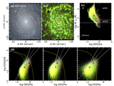
Figure 5 shows the last case of our illustration of the complexity of deriving the nature of the ionization in galaxies. NGC4030 is a grand design Sbc galaxy observed almost face-on. Its disk shows hundreds of HII regions easily identified in the emission-line image (middle-top panel in Figure 5) as green clumpy ionized regions. As expected, most of the ionization is located below the K01 demarcation line (with a large fraction below the K03). However, contrary to examples discussed before (MCG-01-04-025, UGC1395 and ESO298-28), the distribution does not follow the classical location of HII regions. Certainly, a substantial fraction of the line ratios are located in between the K03 and K01 region, and even above the K01 curve in the classical BPT diagram. Following the usual and broadly accepted interpretation of this diagram, this shift should be due to mixing of the ionization produced by the overlap of the HII regions with other ionizing sources that pollute those line ratios (either by a central AGN or DIG due to hot evolved stars, e.g. Davies et al. 2016; Lacerda et al. 2018). However, a more detailed exploration indicates that the polluting sources correspond to clumpy ionized structures, morphologically similar to HII regions, but with line ratios corresponding to the presence of a harder ionization. Those regions clearly correspond to those regions with higher [NII]/H𝛼 line ratios, previously detected in the central regions of galaxies (Kennicutt et al. 1989; Sánchez et al. 2012b), usually referred to as nitrogen enhanced regions (Ho et al. 1997; Sánchez et al. 2015). Recent explorations have shown that they are compatible with supernova remnants combined in some cases with ionization by young hot stars (Cid-Fernandes et al., submitted). Thus, again, the intermediate region can be populated without invoking an AGN to explain the mix of ionization.
In summary, gas in galaxies could be ionized by many different physical processes, as is the case of our own galaxy. Therefore, to associate a single ionization to the observed emission across an entire galaxy is a first order approximation that can lead to considerable errors, in particular in the derivation of the physical parameters of the ionized gas, like dust attenuation or oxygen abundance (due to the non linearity of the combination of line ratios). Furthermore, our ability to distinguish between the different ionization conditions should not rely on the classical diagnostic diagrams only. They should be combined with morphological and kinematic information about the emission line structures and complemented with the study of the properties of the underlying stellar populations to determine their potential ionizing sources. This highlights the fundamental importance of integral field spectroscopy in the study of the ionized gas in extragalactic sources. However, these data are also limited by their spectral and, in particular, their spatial resolution, which can produce a mix of ionization (e.g. Davies et al. 2016) and limit our understanding of the derived properties (e.g. Rupke et al. 2010; Mast et al. 2014).
4.3.Ionized Gas: A Practical Classification Scheme
Based on the results outlined before, we propose a new procedure to classify the components of the ionized ISM. To illustrate it we present in Figure 6 a scheme of the distribution of the most dominant ionization conditions for different galaxy types. We consider that this classification procedure is valid for spatially resolved spectroscopic data between a few hundred pc to a few kpc scales. However, it may not be valid for smaller scales, where the ionization structure is resolved for the different conditions described in the explored data.
A star-forming region is observed as (i) a clumpy/peaked region (clustered) in the ionized gas maps of a galaxy with (ii) line ratios below the demarcation line in at least one of the classical diagnostic diagrams shown in Figure 2 (and Figures 3, 4, and 5), with (iii) EW(H𝛼) above 6Å (see Figure 6, in particular Panels 1 and 2), and with (iv) a fraction of light assigned to young stars (Age < 100 Myr), in the V −band of at least 4-10%. This definition is valid for giant regions and region clusters at the indicated resolution. Small HII regions, like the Milky Way’s Orion Nebula, would be spatially and spectroscopically diluted, and confused with the diffuse gas. In other words, this classification scheme guarantees that the selected regions are indeed ionized by young stars, but it cannot guarantee a complete selection of all regions with the presence of young ionizing stars. Higher spatial resolution data, covering bluer wavelength ranges (UV) would improve this selection process.
An AGN ionized region is observed as (i) a central ionized region (almost unresolved to the considered resolution), well above the intensity of the diffuse ionized gas (Figure 6, Panel 2 and 3, and Figure 3, top-right panel). (ii) Its emission line ratios are above the K01 demarcation lines in the three diagrams discussed before, and (iii) its EW(Hα) is above 3Å (6Å for strong AGN Cid Fernandes et al. 2010). Below that limit it is not possible to determine if the ionization is due to an AGN or to other processes (post-AGBs/HOLMES, low-velocity shocks, photon leaked from regions). They (iv) present a decrease of the considered line ratios with respect to the central values in the galaxy, and (v) show a steep decay in the flux intensity, which is never shallower than an r-2 distribution .
Diffuse gas ionized by hot, evolved stars is seen as (i) a smooth (not clumpy or filamentary) ionized structure that follows the light distribution of the old stellar populations in galaxies. (ii) The EW(Hα) in these regions is clearly below 3Å, with (iii) the fraction of young stars never larger than 4%. (iv) The distributions in the diagnostic diagrams cover a wide range of values from the LINER-like area towards the range covered by metal-rich regions (see Figure 6, panel 3). (v) This component is observed in galaxies with old stellar populations (massive, early types, e.g., Figure 4, left panel) or regions in galaxies with the same characteristics (bulges, Figure 3, bottom-left panel). (vi) The kinematics of this ionized gas does not deviate significantly from that of the old stellar population in the galaxy. Two caveats: In high spatial resolution data (10-100 pc) this component may present, in some cases, clumpy structures associated with individual sources. This is not visible at the resolutions considered in this review. Also, as indicated before, the signal from small-size HII regions is diluted at these resolutions by the ubiquitous DIG emission, which could alter the observed line ratios.
Diffuse gas due to photon-leaking by HII regions is observed as (i) a smooth ionized structure present in galaxies with young stellar populations (in general, low mass and late-type galaxies) or regions in galaxies with the same characteristics (disks, e.g. Figure 6, Panel 1 and Figure 3, greenish diffuse ionization shown in the emission line image located at the disk of the four galaxies). This component should (ii) have a fraction of young stars never larger than 4% within the same resolution element and at the considered resolution (e.g. Espinosa-Ponce et al. 2020). (iii) Its kinematics are not fundamentally different from those of the disk. In the diagnostic diagrams this component may present varying line ratios, from very similar to regions to significantly different from them (e.g. Weilbacher et al. 2018). It also covers a wide range of EW(Hα). Caveats: In high spatial resolution data (10-100 pc) it may present some shells or bubble-like structures, not visible at the considered resolutions. In late spirals (Sc/Sd), it may be the dominant or at least a large fraction of the DIG (e.g. Relaño et al. 2012). In this case, this component should be included in the photon budget to derive the SFR in galaxies (e.g. Zurita et al. 2000).
A high-velocity shock ionized region is seen as (i) a filamentary or bi-conical ionized gas structure with fluxes (and EWs) well above those of the diffuse ionized gas. Its emission line ratios cover a wide range of values. In general, (ii) the line ratios are above the K01 demarcation line in the three diagrams, and (iii) in most cases, the lines are asymmetrical, with (iv) a clear increase of the line ratios (in particular [/H𝛼]) with the velocity dispersion and the distance from the source of the outflow. In addition (v) they have an EW(H𝛼) above 3Å. (vi) This component is usually located in the central regions (or emanating from this region), for both star-formation driven (Hα, Panel 5, and Figure 3, bottom right panel) and/or AGN driven outflows (Figure 6, panel 6). Caveats: The line ratios can spread from the area usually associated with AGN ionization (top-right region of the diagram), to the area covered by HII regions (i.e., below both demarcation lines, and spread through the so-called mixed region). A demarcation line has been proposed to separate between SF and AGN driven outflows , although this should be tested using large/statistically significant samples .
A low-velocity shock ionized region shares many of the characteristics of the DIG by old, evolved stars, and indeed it is considered by different authors as part of this diffuse gas component (e.g. Dopita et al. 1996; Monreal-Ibero et al. 2010). However, these regions present (i) a clear filamentary structure (Figure 6, panel 4), and (ii) a velocity distribution not following the general rotational pattern of the galaxy. The recently named Geyser-galaxies or the cooling flows observed in ellipticals (in clusters in general) show most probably shock ionization corresponding to this type (e.g., Figure 4, right panel).
Supernova remnants are less frequent than in the previous types; they are observed (i) at this resolution as clumpy/ionized regions, similar in shape to the giant regions/star-forming areas discussed before. However, they (ii) are ionized by a harder ionization spectrum and therefore show higher values for the line ratios shown in the classical diagnostic diagrams. Caveats: At the current resolution this component is hard to see without considerable contamination by adjacent or superposed (through the line of sight) HII regions or photon leaking ionized DIG. For this reason they cover a wide range of line ratios, from the classical location of HII regions to the intermediate region between the K03 and K01 regime. In the emission line maps presented in this review this component may appear as reddish clumpy structures (e.g., Figure 5). In general it is required to explore other emission lines, frequently associated with SN and SNR , to detect them (e.g., Cid-Fernandes et al. submitted).
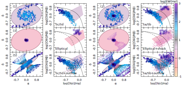
Fig. 6 Scheme of the main ionizing conditions typically observed in galaxies of different morphological types, including both the distribution across the optical extent (left) and the classical BPT diagram (right): (1) late-type spirals (Sc/Sd), without a prominent (or without) bulge. Their main morphological feature is a thin disk (ellipse) together with the spiral arms (dotted line). The main components of the ionized ISM are the HII regions distributed mostly in the disk and following more or less the spiral structure (blue solid-circles), together with some diffuse ionized gas that, in this case, is dominated by photons leaked from those regions (represented as a pale pink ellipse). (2) Early-type spirals (Sa/Sb), with a prominent and well defined bulge, in addition to the disk and spiral arms. They present HII regions and diffuse ionized gas in the disk too, like late spirals. However, the DIG is ionized by a mix of photon leaking and ionization by hot evolved stars, mostly associated with the presence of old stellar populations (i.e., more clearly observed in the bulge, shown as a pink central ellipse). Some also show ionization due to AGN, mostly located in the central regions (violet stars). (3) Early-type galaxies (E/S0), with very weak or no disk. Ionization across their optical extent is dominated by hot evolved stars (pink ellipse), that ionize the diffuse gas, with the possible presence of a central AGN. (4) Early-type galaxies may present shockionized gas, observed mostly in central galaxies in clusters, radio-galaxies, and weak AGN (e.g., like in the case of Geyser galaxies, Roy et al. 2018a). The structure of these relatively low-velocity shocks is filamentary, with a velocity dispersion slightly larger than the one observed in the diffuse ionized gas), and with kinematics largely decoupled from those of the stellar populations in these galaxies. (5) Late-type spirals may present galaxy scale shock ionization associated with galactic winds, which can usually be seen in edge-on or highly inclined galaxies. They show a patchy filamentary distribution, following a conical or biconical structure, emanating from the central regions and escaping to high altitudes with respect to the disk height in some cases. (6) Early-type spirals may show the same kind of galactic winds, but in this case they can be produced by the kinetic energy injected by an AGN too. When observed at high inclination the ionization in the vertical direction can be associated with old stellar populations either in the bulge or a thick disk (not shown in the figure). This latter ionization is less patchy, more diffuse. In all panels, colors represent the typical EW(Hα) associated with the different ionization conditions. The color figure can be viewed online.
We present this classification scheme as a practical tool, with the hope to improve on current classification methods. However, it is by construction incomplete and will require future revisions based on the improvement of our understanding of the ionization conditions observed in galaxies.
5.Global and Resolved Relations
One of the main results emerging from IFS-GS, as highlighted by , is that the global relations uncovered in the exploration of extensive properties of galaxies show local/resolved counterparts that are valid at kiloparsec scales. Among them, the most evident ones are:
The star-formation main sequence (SFMS, e.g. Brinchmann et al. 2004; Renzini & Peng 2015), that relates the SFR and the 𝑀 ∗ for SFGs, has a resolved version that relates the ∑SFR and the ∑* for SFAs (rSFMS, e.g. Ryder 1995; Sánchez et al. 2013; Cano-Díaz et al. 2016; Hsieh et al. 2017; Cano-Díaz et al. 2019).
The mass-metallicity relation (MZR, Tremonti et al. 2004), that relates the central and/or characteristic gaseous oxygen abundance, 12+log(O/H), of a galaxy with its M*, is reflected in the relation found between the local (spatially resolved) oxygen abundance and the mass surface density ∑* in star-forming regions (rMZR, e.g. Rosales-Ortega et al. 2012a; Barrera-Ballesteros et al. 2016).
The scaling relation between the molecular gas mass and the stellar one , corresponds to the recently reported relation between ∑gas and ∑* (e.g. Lin et al. 2019; Barrera-Ballesteros et al. 2020). Because of its similitude with the SFMS, we will refer to this relation as the mass gas main sequence, or MGMS, and to its resolved version as rMGMS, following Lin et al. (2019).
In addition to all these extensive relations and their local/resolved intensive counterparts, recent IFS-GS have allowed to explore in detail well-known relations, like the Schmidt-Kennicutt relation (SK-law, Kennicutt 1998). The SK-law was formulated as a relation between intensive quantities, connecting the average ∑SFR and the average ∑gas across the optical extent of galaxies. However, in principle it was also a global relation, since it relates characteristic properties of individual galaxies. Much work has gone into investigating the true nature of the SK-law, in particular concerning the spatial scales over which it holds and the phases of the neutral ISM which provide the tightest relation. A consensus has emerged in which the SK-law is tightest when relating SFR to molecular hydrogen H2 over scales of a few hundred parsec (e.g. Bigiel et al. 2008, 2011). The advent of IFS-GS, in combination with spatially resolved explorations of the gas content, has allowed to confirm that relation over statistically large samples at kiloparsec scales (e.g. Bolatto et al. 2017). For nomenclature consistency we refer to the resolved SK-law as rSK-law.
It is important to note here that these relations are valid either for SFGs (global) or star-forming areas (SFAs, local/resolved). Retired galaxies (and retired areas) do not follow those relations, showing in general much lower values of the SFR (∑SFR) and Mgas (∑gas) for a fixed M* (∑*), and slightly lower values of SFR (∑SFR) for a fixed Mgas (∑gas). Whether those RGs (and RAs) follow well defined trends or are distributed over extended loci (clouds) in each diagram, is under debate (e.g. Hsieh et al. 2017). Regarding the MZR (rMZR), it is difficult to determine if they follow the same trends or not, since the gas-phase metallicity is very hard to obtain for RGs (RAs). In the few cases in which a globally retired galaxy presents a few SFAs (e.g., Gomes et al. 2016a), it seems that those regions have a slightly lower oxygen abundance than predicted from the relation (Sánchez 2020). However, more statistics are required in this regards.
There are two possible ways to look at the evidence connecting the resolved/local relations with their global counterparts. First, concerning the MZR, theoretical investigations seems to imply that chemical evolution is not dominated by local processes only, but that transport of gas and metals plays a significant role in the physical origin of the relation (e.g. Trayford & Schaye 2019). Similar arguments could be made invoking radial migration, accretion and merging when it comes to the rSFMS. However, the second way to look at the relations is purely empirical, to investigate whether they are at least interchangeable in terms of their intensive vs. extensive nature (e.g. Barrera-Ballesteros et al. 2016; Gao et al. 2018; Sánchez Almeida & Sánchez-Menguiano 2019). Indeed, we will show in the next section that the extensive/global relations are in general a natural consequence of the intensive/resolved ones, while the reverse is not true. While this does not yet make up a proof of which physical processes shape those relations, it becomes probable that most processes surrounding star formation and metal enrichment in galaxies are predominantly local, while global processes only perturb, but do not fundamentally alter, the resulting relations.
In the following we investigate two topics: (i) we transform the global extensive relations into intensive ones, by deriving the average surface densities of the involved quantities Kennicutt 1998). Then we compare the intensive global relation with the local/resolved one; and (ii) we explain with simple calculations why a resolved relation directly leads to an intensive global one, following Sánchez Almeida & Sánchez-Menguiano (2019).
5.1.The Intensive Global Relations
As indicated above, the global scaling relations involve extensive quantities (in most cases), relating often the stellar mass (or gas mass) to other properties of galaxies, such as the SFR, oxygen abundance, of both properties between themselves. As described before, those relations could be a pure consequence of a scaling between galaxies, since they involve pure extensive quantities: the larger and more massive a galaxy is, the higher are the values of any other extensive property, such as the SFR or the gas mass (at least for SFGs). The MZR is slightly different in this regard, since it involves an extensive quantity ( 𝑀 ∗ ) and an intensive one (the oxygen abundance). However, in many cases it is ill-defined, since it is well known that the oxygen abundance shows a radial gradient in galaxies (e.g. Sánchez et al. 2014, and references therein). Furthermore, the oxygen abundance is frequently estimated using variable physical apertures in galaxies, rather than a fixed aperture or a characteristic radius (see Sánchez et al. 2019b, for a recent discussion on the topic). Thus, although the MZR involves an intensive quantity, it is measured as an extensive one (i.e., not averaged across the extension of galaxies). However, it is true that in this particular case the simple scaling of the two parameters due to their extensive nature cannot explain this relation (see the discussion in the seminal article by Tremonti et al. 2004)
We attempt to explore the existence of intensive global relations (rather than extensive ones), by deriving the average surface densities of the considered extensive parameters ( 𝑀 ∗ , Mgas and SFR), and the characteristic value of the oxygen abundance (i.e., the value at the e_ective radius, following Sánchez et al. 2013). To that end we divide each extensive quantity by the effective area of each galaxy, defined as the area within 2re, i.e., Ae=π (2 re)2. We choose this particular radius because most of the IFS data explored in this review sample the galaxies up to this galacto-centric distance. Therefore, most of the reported extensive properties are actually aperture-limited values corresponding to that radius. How the actual parameters were derived, both global and resolved, is described in detail in § 3.
We will demonstrate in the upcoming section that indeed the average intensive parameters derived as described before scale with the corresponding value at the effective radius. For this reason, the current results would be qualitatively similar to the ones found assuming a different scale-length for the galaxy. Finally, for the oxygen abundance we fit its radial gradient, normalized to the effective radius, within 0.5-2 re with a simple linear profile (following Sánchez-Menguiano et al. 2018). Then, we derive the value at the effective radius using the best fit profile for each galaxy.
Figure 7 shows the result of this experiment. In each panel we show, in color-code, number density distributions of the intensive global parameters defined before (and the characteristic one, in the case of the oxygen abundance), including: (i)
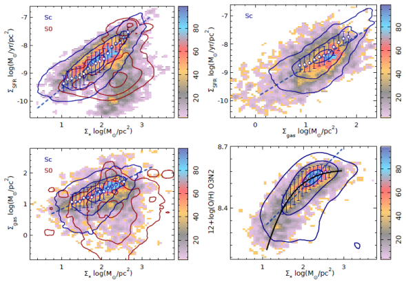
Fig. 7 Global and local (resolved) scaling relations compared. Top-left panel: number density distribution of galaxies in terms of mean ∑SFR against mean ∑* for entire galaxies within our compilation. The distributions are shown as color coded images, where the color bar indicates the cumulative distribution as a fraction of total. In addition, we show the number density distribution of ∑SFR vs. the ∑* for each individual spaxel of each individual galaxy as contour plots, for both the Sc (blue contours) and S0 (red contours) galaxies within the compilation. Each contour encircles 85%, 50% and 10% of the sample, from the outermost to the innermost one. Solid white circles represent the average value of ∑SFR for bins of ≈0.1 dex in ∑*, for galaxies of type Sc, and for those values encircled by the 85% distribution contour, with error bars corresponding to the standard deviation within each bin. The blue dashed line represents the best linear regression to these average points. Top-right panel: Similar plot for the galaxy averaged and spaxel-wise ∑SFR against ∑gas distribution. In this case, for the resolved properties we only show the contours corresponding to Sc galaxies. Bottom-left panel: Similar plot for the ∑gas-∑* diagram. Bottom-right panel: Similar plot for the distribution of oxygen abundance vs. ∑*. In the last case, the contours correspond to the number density distribution of all the spaxels with measured oxygen abundance for the full sample of compiled galaxies (black contours); although in practice, it contains mostly late-type, star-forming galaxies. In this panel a best fitting curve is included as a black solid-line, following the functional form usually adopted to describe the relation between these two parameters, first proposed by Sánchez et al. (2013). The color figure can be viewed online.
The second panel (∑SFR-∑gas diagram) shows the well known SK-law for the analysed sample. Like in the case of the SFMS, the well known trend between the two parameters is visible, despite the fact that we are using a proxy to estimate the gas content, based on the dust attenuation (Barrera-Ballesteros et al. 2020), as discussed in § 3.2. The third panel (∑gas - 𝛴 ∗ diagram) mimics the known relation between the gas and the stellar mass, for SFGs, with a tail towards lower values of Mgas (∑gas in this case) for retired galaxies (e.g. Saintonge et al. 2016; Calette et al. 2018; Sánchez et al. 2018; Lacerda et al. 2020). Finally, the fourth panel shows the intensive version of the MZR diagram, thus, the distribution of the characteristic oxygen abundance of each galaxy (i.e., the value at re) against the average
The main goal of this exploration is not to discuss the physical origin of the reported relations. For that discussion we refer to Sánchez (2020), where the different relations are described in more detail. In this particularly case we are just interested in showing that the global relations, here expressed in their intensive form, do actually correspond to the local/resolved ones reported in the literature. For this reason we overplotted in the different diagrams the corresponding local/resolved distributions for the individual spaxels within our compilation of IFS data. When required, we plot the distributions segregated by morphology, since in many cases the reported relations depend on the morphology (as discussed before), being in general different for star-forming galaxies (dominated by late-type galaxies) than for retired galaxies (dominated by early-type ones) (e.g. Lacerda et al. 2020). Panel by panel we can see that the resolved distributions for SFGs (represented by Sc galaxies) follow exactly the same trends as the global intensive properties for the ∑SFR-∑*, ∑SFR-∑gas and ∑gas-∑* diagrams. Similar results are found when using a different estimator for the gas mass density, as the one described in § 3.2 (labeled as
We perform a linear regression between the different parameters shown in Figure 7 to characterize the relation between them. For this analysis we derive the mode of the distribution along the y-axis in a set of bins of ≈0.1 dex along the x-axis for each diagram, for those values encircled by the 80% density contour in Figure 7. The points derived this way are represented as solid white circles in the figure. Then we perform a least-squares regression based on a Monte-Carlo procedure, with the best fit parameters and their errors derived as the mean and standard deviations of the reported parameters in each iteration. This procedure is very similar to the one adopted by similar recent explorations (Sánchez et al. 2019b; Barrera-Ballesteros et al. 2020). The result of this procedure is included in Table 1, together with values reported in the literature. In general, there is good agreement between the current reported trends and values in the literature. This is particularly true for the ∑´gas estimation of the gas mass density (in the relation involving this parameter, i.e., rSK and rMgM*). The dispersion around the main trend, characterized by the standard deviation, is also of the same order or smaller than the one reported in the literature. In the case of the rMZR we included a linear regression for consistency with the other explored relations. However, it is well known and it is clear from inspection of Figure 7 that this functional form does not describe the distribution along the full range of explored parameters. Other functional forms, like a higher order polynomial function (Rosales-Ortega et al. 2012b) or a linear+exponential one (Sánchez et al. 2013), better describe this distribution. For this reason we include in the figure the best fit curve using this latter model, with the functional form:
where x is log(
Table 1 Log-log fitting to resolved relations
| Relation | Reference | β | α | rc | σ |
| rSFMS | This work | -10.35±0.03 | 0.98±0.02 | 0.96 | 0.17 |
| Sánchez et al. (2013) | 0.66±0.18 | 0.66 | |||
| Wuyts et al. (2013) | -8.41 | 0.95 | |||
| Cano-Díaz et al. (2016) | -10.19±0.33 | 0.72±0.04 | 0.63 | 0.16 | |
| Lin et al. (2019) | -11.68±0.11 | 1.19±0.01 | 0.25 | ||
| Cano-Díaz et al. (2019) | -10.48±0.69 | 0.94±0.08 | 0.62 | 0.27 | |
| rMGMS | This work using ∑gas | 0.24±0.04 | 0.60±0.02 | 0.93 | 0.08 |
| This work using ∑´gas | -1.10±0.07 | 1.22±0.03 | 0.95 | 0.14 | |
| Lin et al. (2019) | -1.19±0.08 | 1.10±0.01 | 0.20 | ||
| Barrera-Ballesteros et al. (2020) | -0.95 | 0.93 | 0.20 | ||
| rSK | This work | -9.85±0.02 | 1.19±0.02 | 0.96 | 0.11 |
| Using ∑´gas | -10.72±0.04 | 1.17±0.02 | 0.97 | 0.15 | |
| Bolatto et al. (2017) | -9.22 | 1.00 | |||
| Lin et al. (2019) | -9.33±0.06 | 1.05±0.01 | |||
| rMZR | This work | 8.21±0.01 | 0.13±0.01 | 0.88 | 0.06 |
Results for the log-log regressions between the different parameters shown in Figure 7, with β being the zero-point of the relation, α the slope, rc the correlation coefficient between the involved parameters and σ the standard deviation around the best fit relation. We include similar results extracted from the literature, shifted when needed to match the adopted units for the different quantities. We remind the reader that our surface density quantities are all expressed in units of pc2 for the area. (1) We should note that the Wuyts et al. (2013) results are based on galaxies at z ≈ 1. Thus, the offset in β reflects an evolution in the rSFMS similar to the one reported for the SFMS (e.g. Speagle et al. 2014; Sánchez et al. 2019a).
The distributions shown in Figure 7 clearly demonstrate that the rSFMS, rSK and rMGMS resolved relations are indeed the same relations as the intensive versions of the SFMS, SK and gas-stellar ones. Even more, the individual spaxels of the RGs (represented by S0 galaxies in here), are located off and below the reported relations for the SFGs in the ∑SFR-∑* and ∑gas-∑* diagrams, following exactly the same trends as those reported for the RGs. Finally, the rMZR distribution for the bulk sample of galaxies follows exactly the same distribution as the intensive version of the MZR. This distribution is always dominated by SFGs, since they are the only ones were the oxygen abundance is properly derived.
This exercise shows that the global and local/resolved relations are indeed the same relations, covering the same ranges, following the same distributions (and trends) and the same morphological segregation (in general). We should note, however, that selecting SFGs and RGs is not exactly the same as selecting star-forming areas (SFAs) and retired-areas (RAs), as recently discussed by Cano- Díaz et al. (2019). There are RAs located in (mostly the center) of SFGs, and also a few SFAs located in (mostly the outer part) of RGs (e.g., Singh et al. 2013a; Gomes et al. 2016b; Belfiore et al. 2017a). This should surely affect the global (intensive or extensive) relations, since they deal with average quantities, mixing SFAs and RAs within the considered apertures. Despite this caveat we stress the remarkable agreement between the explored global and resolved relations.
5.2.Universality of the Local Relations
One relevant question regarding the local relations explored in the present section is their universality. In other words, whether the resolved regions of different galaxies lie along the same reported relation, irrespective of the properties of the host galaxies (global or local), or, on the contrary, if part of the dispersion reported in those relations is the consequence of the existence of different relations for different families of galaxies (or possible secondary correlations). In global relations this exploration has led, for instance to the extensive search for a third parameter to explain (or reduce) the scatter in the SFMS and the MZR relations (SFR, gas fraction, e.g. Mannucci et al. 2010; Bothwell et al. 2013). It has also led to a debate over the need for that third parameter (e.g. Sánchez et al. 2013; Barrera-Ballesteros et al. 2018). Regarding the local/resolved relations, similar explorations were recently performed by Barrera-Ballesteros et al. (2016), Cano-Díaz et al. (2019) and Ellison et al. (2020), in the case of the rMZR, rSFMS and rSK (resolved SK-law), respectively. They find that: (i) it is not clear that a secondary parameter is required to explain the dispersion in the rMZR (in particular the ∑SFR; (ii) galaxies of different morphologies and SFE segregate both the SFMS and the rSFMS ; and (ii) stellar mass and SFE segregate the rSK (see also Bolatto et al. 2017; Colombo et al. 2018). This was already discussed in in detail, describing the similarities and differences for different stellar masses and morphologies. The rMZR was not included here, since it clearly requires a more complex parametrization. In order to present a more quantitative evaluation of the variation of the different local relations with global properties of galaxies we repeat the linear regression to the rSFMS, rMGMS and rSK relations discussed in the previous section segregated in bins of mass and morphology. rMZR was not included here since it clearly requires a more complex parametrization
We adopted the same bins as those described in , including four ranges of stellar mass (M = 107.5-109.5, 109.5-1010.5, 1010.5-1011 and ), seven morphological types (E, S0, Sa, Sb, Sbc, Sc and Sd), and an additional bin including all morphologies, and the same stellar mass bins (labelled as ALL). Figure 8 illustrates the result of this analysis, showing the variation of the zero-point (β) and slope (α) of the linear relations against morphology and stellar mass. The values shown in this figure are contained in different tables available to the community5.
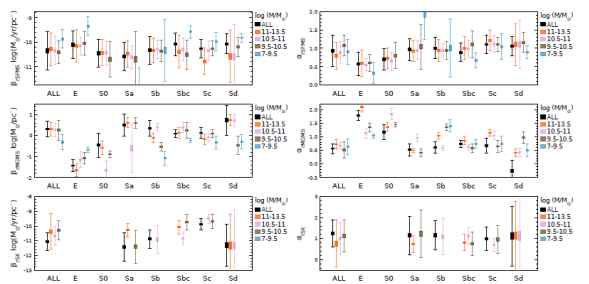
Fig. 8 Top panel: Zero-point of the rSFMS relation derived for different morphology (black symbols) and stellar mass (colors) bins. For each sub-sample the mean value of the considered zero-point is shown, together with the standard deviation (shown as a rectangle) and the minimum and maximum values within the distribution (shown as error-bars). Middle panel: Similar distribution for the slope of the rMGMS. Bottom panel: Similar distribution for the slope of the rSFMS. The color figure can be viewed online.
The distributions confirm the results reported in the literature: (i) the rSFMS presents a mild change with the stellar mass, and a stronger variation with morphology, with SFAs of more massive and earlier galaxies showing a shallower slope in the relation and lower values of the ∑SFR for a given ∑*; (ii) the rMGMS shows clear patterns with mass, but again, even stronger and clearer ones with morphology. SFAs in early-type galaxies have lower values of ∑gas for a given ∑* (i.e., a molecular gas deficit), an effect that is enhanced by the stellar mass (i.e., the gas deficit is stronger in more massive early-type galaxies). The relation between the two mass densities is steeper (larger value of α) than the one reported for their counterparts in SFGs, indicating that the central (more massive) regions of early/massive galaxies may still contain some molecular gas that is scarce in the outer regions . On the contrary, the SFAs of more massive SFGs have an overall higher ∑gas for given ∑SFR than those of less massive SFGs, and a shallower relation between both parameters; (iii) the rSK, which has the noisiest distribution, shows a dependence with mass and morphology that is more evident in the zero-point (or scale) than in the slope (which seems rather constant, with α ≈ 1). This trend indicates that the SFE is lower in SFAs of earlier and more massive galaxies.
Thus, although there are local/resolved relations in galaxies suggesting that the SF processes are governed by physical processes that happen at kiloparsec scales, those relations are not fully universal. Indeed, most probably they are not fundamental, being the statistical effect of physical processes that happen at a much smaller scales(≈10 pc). They show dependencies with the global properties of galaxies that modulate them, indicating a clear interconnection between local and global processes, as also discussed in Sánchez (2020).
5.3.Prevalence of Local Relations
The experiments in previous sections show that local/resolved and global intensive relations are indeed the same relations. However, they do not indicate which of them is prevalent in their physical origin. In other words, they do not show that global relations are just an integrated (averaged) version of the resolved ones. To demonstrate that this is the case, at least mathematically, we should show that once there is a local/resolved relation it is inevitable to generate a global one, but not the contrary. We will now explore this.
It is well known that many of the physical properties in galaxies have a radial gradient at first order. In particular, all the properties described in the previous section do actually show a radial decline for all galaxy types and all stellar masses and morphologies, on average. This is particularly true for the radial distributions of ∑* and ∑gas. In some particular mass/morphological types and for some particular galaxies the radial distribution may be flat of even inverted. This may be the case for ∑SFR and 12+log(O/H), although those are not the general/average trends. If the local relations have a physical prevalence, this means that all radial relations/trends are a consequence of the relations between the explored quantities and ∑*, and the radial dependence of this parameter, i.e., ∑* = F(r). In general, the radial distribution of ∑* is well represented by a log-linear dependence with the galactocentric distance (which we adopt normalized to the effective radius, following Sánchez 2020). At first order it shows an almost universal exponential decline that can be parametrized with the following functional form:
where ∑0 is the stellar mass density in the central regions, reis the effective radius, and b is a parameter that controls the slope of the log-linear relation (with that slope being b´= b/In(10)).
Therefore, if a parameter 𝑝 (e.g., ∑SFR), has a log-linear relation with ∑*, of the form:
then:
or, in another form:
where p0 =
However, the existence of a radial dependence of
In more detail, let P be the global property corresponding to the resolved property p (e.g., like the SFR to the ∑SFR). In this particular case, we will show that it is possible for P to follow a global dependence with M*, with the same functional form as the local relation shown in equation 8:
without fulfilling a local/resolved relation between p and ∑* . Let us assume that ∑* has a radial dependence described by equation 7, but that p is constant along the extension of a galaxy. Then, no local/resolved relation would be verified, since at different galactocentric distances ∑* would have different values, while p would remain constant. However, if both quantities are integrated up to a particular radius (e.g., r < 2re), then:
and:
then, even if all galaxies had universal ∑0 and p values, both quantities would show a similar dependence with the effective radius, and they would show a global relation similar to the one indicated before.
It is true that this is a very particular case, and it is totally unrealistic. However, it illustrates that the presence of a global relation does not guarantee the existence of a local/resolved one. The converse, on the other hand, is not possible. If galaxies present a local relation between parameter p and ∑* in the form described by equation 8, then galaxies would present a global relation as the one described by equation 11. To demonstrate this, we use the results of equations 13 and 10 to show that in this case P would be:
and recalling the definition of p0, and b´, and equation 13 then:
where
and
Since the effective radius re has an almost log-linear scaling relation with M* (e.g. Sánchez 2020, and references therein), following a similar functional form as equation 11:
then:
and therefore the proposed extensive global relation is verified (i.e., we recover naturally equation 11).
Furthermore, even when the relation shown in equation 16 is not verified, an intensive global relation holds. If we define the intensive global quantities
which it is indeed a global relation between intensive quantities that mimics the local one. In particular, it has the same slope as the local one, with a slightly different zero-point, when represented in a log-log form. We should highlight here that the zero-point of this relation is not a dimensionless quantity, and particular care should be taken when the surface densities are expressed in different areal units (e.g., when transforming between pc-2 or kpc-2, if the value of d is not one). These are the relations that match the local/resolved ones, as shown in Figure 7. In principle, the scale/zero-point are different by a factor B-dD between local and global intensive relations. However, adopting the average values reported for those relations, shown in Table 5, we found that the expected offset is ≈0.05 dex, being compatible with zero in some cases (like the rSK and rSFMS relations).
Finally, we should stress that if local relations segregate by morphological type (or other properties of galaxies), then global ones should also segregate, depending on the particular effect in the scaling of the zero-point. This effect should be stronger for the extensive global relations, which depend on the relation between the effective radius and the stellar mass shown in equation 16. It is known that this relation is different for early- and late-type galaxies. Therefore, even if both families show the same local/resolved relations, their global extensive ones should segregate just due to this effect, without involving different physical processes. This stresses the need to explore the global relations in their intensive and not in their extensive form, as it is usually done.
5.4.Characteristic Intensive Properties
In the previous sections we studied the existence of global relations between galaxy parameters based on an intensive formulation, rather than an extensive one as customary in the literature. We used average surface densities within 2re in galaxies. In the case of the oxygen abundance, we adopted the value at re as the characteristic oxygen abundance for a galaxy. Previous studies have indeed reported that the values of many different quantities at this particular radius are representative/characteristic of the average quantity across the optical extent in galaxies (e.g. oxygen abundance, stellar ages and metallicities, stellar mass density, Sánchez et al. 2013; González Delgado et al. 2014; García-Benito et al. 2017). This is indeed a corollary of the derivations in the previous section, as we will see here.
We assume again that P is a global extensive quantity, and that it results from the integral of the corresponding surface density p across the optical extent of a galaxy, as described in the previous section. A radial distribution described by equation 14 follows. Then, with equation 10 and the definition of
Then, defining pe as the value of p at the effective radius, it is possible to derive the relation:
Thus, the average value of the surface density across the optical extent (r < 2re) is related to the value at the effective radius by a multiplicative constant that depends only on the slope of the radial gradient. Indeed, in the case of b´≈ 1, i.e., an exponential profile,
6.Characteristic Gradients of Resolved Properties
So far, we have demonstrated that the existence of a local relation between an observed property and ∑* implies that this property has a radial gradient (if ∑* has that gradient originally, as shown by Barrera-Ballesteros et al. 2016). The radial gradients of all the properties explored in the previous sections do indeed exist and were extensively discussed in Sánchez (2020). It was shown that in general, most of those properties show indeed a radial decline. This decline is frequently characterised to first order with an exponential function (as indicated in the previous sections), i.e. a log-linear function. Fitting that function to the observed distributions it is possible to derive the corresponding value of each considered parameter at the effective radius (which is representative of the average value), plus the magnitude of the radial gradient/slope of the radial gradient, either galaxy by galaxy, or averaged by galaxy type.
This analysis has been frequently performed to explore whether the proposed radial distributions (and therefore the local and global relations, as demonstrated in the previous sections) are universal (i.e., essentially the same, not dependent on other galaxy properties) or if they depend on the properties of the galaxies (e.g. morphology, mass, star-formation rate, gas content). In this particular section we report on the log-linear fitting performed on the average radial profiles of the properties explored by Sánchez (2020)) in different mass bins and morphological types. We use the same bins described in that article, including four ranges of stellar masses (M=107.5-109.5, 109.5-1010.5, 1010.5-1011 and 1011
where 𝛼 is the slope of the gradient (related to the b´ parameter of equation 10) and β is the zero-point. From this relation it is possible to derive the characteristic value (i.e., the value at re), which would be
In order to avoid possible resolution problems affecting the central regions of the galaxies and to truncate to a radius covered by all IFS data, we restricted the fitting to the radial range between 0.5 and 2.0 re. Like in the case of the local relations explored in § 5.2, we repeat the analysis for galaxy subgroups segregated by mass and morphology, following Sánchez (2020). The results of the analysis are included in the electronically distributed tables.6
Figures 9 to 16 present the results of this analysis, showing the distribution of the characteristic value (e.g.,
Stellar mass density gradients: Figure 9 shows that the characteristic stellar mass density has a clear dependence with the integrated stellar mass (M*), as a consequence of the relation shown in equation 13. In this way

Fig. 9 Top-panel: Characteristic value of 𝛴 ∗ at the effective radius for all galaxies in the sample (black symbols), and for different stellar masses (colors) and different morphologies. For each subsample we show the mean value of the considered parameter, together with the standard deviation (shown as a rectangle) and the minimum and maximum values within the distribution (shown as error-bars). Bottom-panel: Similar distribution for the characteristic slope of the radial gradient of the 𝛴 ∗ parameter. The color figure can be viewed online.
It is worth noticing that the most massive E-type galaxies are not the ones with the largest
Age and metallicity gradients: Figure 10
and 11 show the distributions of the
luminosity weighted (LW) characteristic ages and metallicities of the stellar
populations together with the slope of the radial gradients. For both parameters
similar trends are found, with earlier and more massive galaxies showing older (

Fig. 10 Same as Figure 9, but for the luminosity-weighted ages of the stellar populations. The color figure can be viewed online.

Fig. 11 Same as Figure 9, but for the luminosity-weighted stellar metallicity. The color figure can be viewed online.
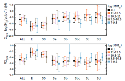
Fig. 12 Same as Figure 12, but for the star-formation rate surface density 𝛴 𝑆𝐹𝑅 . The color figure can be viewed online.
Star-formation density gradients: Figure 12
shows the distribution of characteristic values and gradient slopes of the
star-formation surface densities for the different morphological and stellar mass
bins. As expected, early type galaxies (E/S0) show lower
Similar trends are reported for the radial distribution of the specific star-formation rate, as shown in Figure 13, with clearer and sharper distributions as a consequence of the combination of
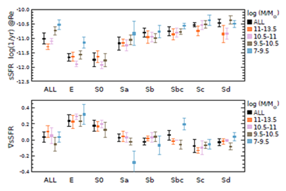
Fig. 13.Same as Figure 9, but for the specific star-formation rate. The color figure can be viewed online.
Similar results are found when other estimators for the SFR are adopted. In particular, in the case of the SFR derived using the stellar population analysis described in § 3.1 the results are totally compatible with those described here. We provide the corresponding measurements in the distributed tables, although no figures are provided to avoid repetition.
Gas density gradients: Figure 14 includes
the distributions of the characteristic values and the radial gradients for the
molecular gas mass surface density for the considered sub-samples. We should stress
out that this derivation was obtained based on the dust-to-gas calibrator presented
in Barrera-Ballesteros et al. (2019) (as
described in § 3.2). Like in the previous properties, there are clear trends, with
more massive galaxies showing more gas (

Fig. 14 Same as Figure 9, but for the molecular gas mass surface density 𝛴 𝑔𝑎𝑠 . The color figure can be viewed online.
Regarding the slope of the radial gradient, the trends are more complicated than the ones described so far. On average, when all morphologies are included, the slope for late type galaxies is almost constant , without a clear trend with stellar mass. However, early type galaxies show a sharp negative gradient (
In general these results indicate that RGs have a global lack of molecular gas, as discussed by Saintonge et al. (2016) and Sánchez et al. (2018). Furthermore, they show a deficit that is stronger in the inner regions than in the outer ones, which suggests that the inside-out quenching process (e.g. González Delgado et al. 2016; Belfiore et al. 2017b), is driven also by a lack of gas. The fact that quenching seems to be connected with the presence of a central (active) massive black-hole has been frequently proposed in the literature (e.g. Hopkins et al. 2010). Recently explorations using spatially resolved IFS data support this scenario (e.g. Bluck et al. 2019), suggesting that AGN are related with inside-out quenching and the removal (or heating) of gas which is thus prevented from settling as molecular clouds. However, there is no general consensus in this regard, since other recent contributions (e.g. Ellison et al. 2020) indicate that star-formation efficiency could be the primary driver for halting of the SF rather than a real lack of gas. We should be cautious in this regards since most estimations of the spatially resolved molecular gas density, based on CO observations, are biased towards late-type galaxies (e.g., EDGE, ALMAQUEST, Bolatto et al. 2017; Lin et al. 2019), while the current estimations, although indirect, also cover early-types (in particular pure ellipticals), where the strongest drop in
Star-formation efficiency gradients: Figure
15 shows similar plots as the ones described before for the
star-formation efficiency (SFE=

Fig. 15 Same as Figure 9, but for the star-formation efficiency. The color figure can be viewed online.
In addition to this global dependence with galaxy mass and morphology, there are also evident radial differences. On average the SFE presents a gradient with a negative slope of
Oxygen abundance gradients: Figure 16 shows the distribution of the characteristic oxygen abundance and the slope of the corresponding radial gradient for the different stellar masses and morphologies explored in this section. We adopted the O3N2 calibrator proposed by Marino et al. (2013), which imposes certain restrictions/biases regarding the absolute values of the abundances and the range of values covered with each galaxy (see Kewley & Ellison 2008; Sánchez et al. 2019b). However most of the qualitative results are independent of the adopted calibrator (in particular regarding the abundance gradient, e.g. Sánchez-Menguiano et al. 2016, 2018). Another caveat to note is that oxygen abundance is only derived for those galaxies that have SF ionized regions populating the explored spatial range densely enough to derive a reliable gradient. Therefore, the numbers of galaxies in the earliest-type subgroups are really small.

Fig.16. Same as Figure 16, but for the gas phase oxygen abundance derived using the O3N2 calibrator. The color figure can be viewed online.
On average, galaxies in the nearby Universe have an oxygen abundance of 12+log(O/H)≈8.5 dex. However, this is strongly modulated by the stellar mass due to the well known MZR (Tremonti et al. 2004), and the resolved version discussed in § 5. The most massive galaxies show a plateau in the oxygen abundance around ≈8.5 dex, while the less massive ones have values as low as ≈8.3 dex. We remind the reader that the actual absolute values may change from calibrator to calibrator. Furthermore, a trend with morphology is apparent. However, in most of the cases the abundance is very similar among galaxies of the same mass, despite their morphology. Thus, the morphology trend seems to be induced by the mass-morphology and MZR relations, rather than being a real secondary trend. Only for the less massive and latest type galaxies is there some appreciable difference induced by the morphology and not only by the stellar mass.
Regarding the abundance gradient, it was reported that late-type galaxies of mass
7.Discussion and Conclusions
In this manuscript we have reviewed the most recent results based on IFS extracted from recent galaxy surveys following , but including additional details that clarify some of the conclusions presented in that review. We made use of the large collection of galaxies observed with IFS selected for the previous study. All of them were analyzed using the same tool (Pipe3D, Sánchez et al. 2016b), in order to homogenize as much as possible the compiled data. Based on those parameters we explored different spatially resolved and integrated properties of galaxies.
First, we explore the local/resolved nature of the dominant ionization processes in galaxies. Based on this analysis we demonstrate that the use of integrated or aperture limited parameters of the emission lines (line flux intensities and ratios) may produce significant errors in the interpretation of the ionizing sources in galaxies. We show the main trends of the integrated and resolved line ratios with galaxy morphology and masses, illustrating them in detail with a few galaxies observed with the IFU which provides the best spatial resolution so far for a wide FoV (i.e. MUSE). Based on that analysis we update the practical scheme presented in Sánchez (2020) to classify the ionization sources at the spatial resolution considered in this review (∼1 kpc). Our main conclusion is that the location within the classical diagnostic diagrams is not enough to distinguish between the dominant ionizing sources in galaxies. The inclusion of a third parameter, like the EW(Hα), partially mitigates the intrinsic degeneracy in the observed line ratios. The additional use of (i) the knowledge of the composition of the underlying stellar population, (ii) the spatial distribution and shape of the ionized gas, and (iii) a knowledge of the gas kinematics, substantially improves our ability to distinguish between different ionizing sources. However, all this is hampered by the spatial and spectral resolution of the adopted data.
Then, we explore in a more quantitative way the global and local relations that seem to result from the star-formation processes in galaxies (and regions within galaxies) already reviewed in Sánchez (2020): the SFMS, MGMS, SK and MZR relations. We revisit the most recent results in this regard and re-evaluate them using our extensive dataset. The main conclusions of this exploration are that: (i) there are resolved/local versions of the global relations which are verified at kiloparsec scales for SFAs; (ii) those relations are similar in shape to global ones. This is particularly true for the intensive versions of those relations, which totally overlap the resolved/local ones; (iii) global and local relations are verified for star-forming galaxies (and areas/regions within galaxies), but not for retired galaxies (areas). Thus, these relations are tightly related to the star-formation activity. Retired galaxies (areas) follow different trends, which show more lose relations or clouds; (iv) global and local relations are not fully universal: i.e., they are similar but not exactly the same for different galaxy types and stellar masses; (iv) global relations can be derived from local ones with fewer assumptions than the other way around. Indeed, just considering that more massive galaxies are in general more extended (i.e. the existence of a M*-Re relation), the existence of a local relation implies the presence of a global one. The contrary is not true: i.e. it is possible to have global relations without the need for local ones.
All these results suggest that local relations have a physical prevalence over global ones, and that the star-formation is governed by processes that leave clear imprints at kiloparsec scales rather than galaxy- wide. In fact, these processes are likely originated at much smaller scales. They involve most probably the self-regulation introduced by the feedback that modulates the gravitationally driven trend of molecular clouds to collapse and form new stars. The rSFMS and rSK relations, and the dispersion around them, are most probably the result of the bouncing effect of those two processes working one against each other. In this way, the MGMS relation would highlight the ability of the local gravitational potential to hold both components bound to the system. Under this interpretation it is naturally explained that the rSFMS and rMGMS evolve along cosmic times: (i) galaxies (and regions within them) in the past have higher SFRs at a given M* (or Σ*) and (ii) galaxies (and regions within them) have larger amounts of molecular gas. The expected evolution is demonstrated for the rSFMS just by comparing the relation reported at z ≈ 0 (Sánchez et al. 2013) with the one reported at z ≈ 0.7, showing an evolution similar to the one found for the SFMS (e.g. Speagle et al. 2014). Under this scenario the rSK (SK) relation should show a weaker evolution along cosmological times. The same scenario would explain the morphological segregation of the rSFMS and MGMS relations, since later-type galaxies (and SFAs within them) would show a smoother evolution of the rSFMS as a consequence of a smoother star-formation history (e.g. López Fernández et al. 2018).
In this way the dependence (or modulation) of local/resolved relations on global properties of galaxies is naturally explained. The dynamical stage of a galaxy influences the way the star formation happens (or is halted) in different locations, modifying the local relations. The presence of a bulge seems to stabilize the molecular clouds (Martig et al. 2009) and it would be the reason behind the morphological segregation of the SFMS (Catalán-Torrecilla et al. 2017, e.g.) and rSFMS (e.g. González Delgado et al. 2016; Cano-Díaz et al. 2019). On the contrary, local effects, like the over-pressure produced by the passage of a spiral arm, may enhance the SFR locally, producing local fluctuations in the local relations (e.g. Sánchez-Menguiano et al. 2017, 2019). Another interpretation is that the SFMS (and the rSFMS) holds only for the disk (or regions within disks) of galaxies (regions with cold orbits), and the morphological segregation is a consequence of the increase of M* (Σ*) due to the inclusion of stars in warm/hot orbits. This is supported by the recent results by Méndez-Abreu et al. (2019), which show that SFMS holds for the disk component of galaxies once they are spatially decomposed.
Additional global processes, like galactic winds or the presence of an AGN can alter those relations. Physically, it is known that galaxy-wide winds are important for setting galaxy metallicities and even baryonic fractions. In particular, galactic winds are usually claimed to be responsible for the shape of the MZR. The linear rising phase of this relation, observed at M*<10-10
On the other hand, it seems that AGN may be more relevant in the quenching of star-formation activity. The energy injection by these powerful sources is the primary candidate to explain the halt of star formation either by removal or heating of gas (e.g. Hopkins et al. 2010). The location of AGN hosts in the green valley region of galaxies in different diagrams (like the CMD or the SFR- 𝑀 ∗ ), reinforces this perception (e.g. Kauffmann et al. 2003; Sánchez et al. 2004; Schawinski et al. 2014; Lacerda et al. 2020). Nevertheless, quenching is not an instantaneous and coherent process galaxy-wide. It is a local process too, evolving from the inside out (González Delgado et al. 2016; Belfiore et al. 2017a), with AGN hosts being in transition between SFGs and RGs in this regard too (Sánchez et al. 2018). Recent explorations suggest that the presence of a central massive black hole is directly connected with the global and local quenching (Bluck et al. 2019). Thus, again, although the presence of an AGN could be considered as a global process, its effects in the processes and relations are local.
Finally, to be efficient, both processes, galactic winds and AGN, require that the injected kinetic energy equals or exceeds the local escape velocity. For this reason their effect was much stronger in earlier cosmological times, when galaxies were less massive, had larger SFRs, and hosted AGN more frequently. Maybe for this reason their effect seems less evident in the relations and patterns explored in this review, which correspond to those of nearby galaxies. For instance, the metal redistribution usually associated with galactic outflows should have a limited effect in today´s ´s massive galaxies. It is known that massive galaxies exhibit a strong metal enrichment in their early cosmological times (e.g. Vale Asari et al. 2009; Walcher et al. 2015, Camps-Fariña in prep.), in agreement with their known SFHs (e.g. Panter et al. 2007; Thomas et al. 2010). At the same time, they show oxygen abundances (e.g. Sánchez et al. 2013) and stellar metallicity gradients (e.g. González Delgado et al. 2014) that agree with a local downsizing and inside-out growth (e.g. Pérez et al. 2013b). The gradients in their stellar and ionized gas properties, like the ones explored in § 6, are therefore a fossil record of the early evolutionary phases in galaxies. Thus, even in the period of more violent SFRs, and therefore stronger and more frequent outflows, the metal redistribution induced was not strong enough to blur the observed gradient. It is expected that nowadays, when outflows are more scarce and less energetic (Ho et al. 2018; López-Cobá et al. 2019, 2020), their effect is even less prevalent in this regard, at least for massive galaxies.
On the other hand, low mass and late-type galaxies could be more strongly affected by SF driven outflows. Their SFHs, global or resolved, show a smoother cosmological evolution, being still in the rising phase for the lowest mass and latest type galaxies (e.g. López Fernández et al. 2018), with smaller inside-out differences. As a consequence, in those galaxies the signatures of inside-out formation (e.g. radial gradients in the explored properties, § 6), are less evident. This is particularly true for the oxygen abundance and stellar metallicity distributions. As already discussed in Sánchez (2020) those galaxies exhibit a flat or even inverse gradient in these properties, even potentially implying an outside-in growth phase. In general, it can be considered that their overall evolution is delayed with respect to that of more massive galaxies with earlier morphological types.
The influence of galaxy environment on the evolution of galaxies and the observed global and local patterns has been very little discussed in this review (and in Sánchez 2020). The main reason is that galaxy samples currently observed by IFS-GS are still not large enough, or will require a more detailed reevaluation to distinguish the environmental effects. In this regard, the results of the SAMI project (which has by design a large sub-sample of cluster galaxies) and the GASP survey (Poggianti et al. 2017, which explores the gas stripping in galaxies entering into clusters), would be of a particular importance. The comparison between the properties of field and cluster members, or central and satellite galaxies, in large samples, like the one provided by MaNGA, would also provide more insight on this particular problem. However, the current number of these analyses is too limited and they are too recent to make firm conclusions in this regard.
In summary, we review here our current understanding of the interconnection between the local and global properties of the ionized gas and stellar populations in galaxies in the nearby universe. In particular, we discuss the ionization processes and the star formation and metal enrichment cycle in galaxies. The main conclusion, in the same line as the ones presented in , is that these processes are governed mostly by local physical processes which are modulated by global ones. Whether the influence of those global properties is through local ones or not would be a matter of exploration for the next years.

