


![An astrometric and photometric study of the intermediate-age open cluster NGC 2158 and its eclipsing binary [NBN2015]78](/img/es/next.gif)


 nueva página del texto (beta)
 Inglés (pdf)
 Artículo en XML
 Referencias del artículo
 Enviar artículo por email
 Citado por SciELO
  Similares en
SciELO
Similares en
SciELO 
 Permalink
1. INTRODUCTION
The study of the chemical composition of H II regions is crucial for the understanding of the chemical composition of the universe; it can provide observational constraints required by models of galactic chemical evolution. The proper determination of the oxygen abundance in H II regions is critical to be able to compare our determinations with other branches of astrophysics, as well as to be able to present a coherent model of the evolution of the universe.
Although a comprehensive chemical composition is desired, frequently studies are only able to determine a few chemical elements; in fact many works focus only on the oxygen abundance. A single well determined element can be quite useful, since most elements are expected to behave in an orchestrated fashion, and oxygen is the ideal candidate, since it is expected to comprise about half of the heavy element abundance; not only that, but is the easiest element to study since it is the only element that produces bright optical lines for each of its main ionic species.
There are three competing methods to derive ionic O+ and O++ abundances, relative to the H+ abundance, in H II regions: (i) The use of ENT#091;O IIENT#093; and ENT#091;O IIIENT#093; collisionally excited lines (CELs) together with the H Balmer lines; these lines are relatively easy to observe. Unfortunately their emmisivities depend strongly on the local temperature (in fact, this specific characteristic of CELs is used to determine the characteristic temperature of photoionized regions); this is known as the direct method (DM). (ii) The use of O I and O II recombination lines (RLs) together with the H Balmer lines (which are also RLs); this strategy has the advantage that the ratios of any pair of RLs are almost independent of the temperature structure; however, RLs of heavy elements are quite faint and harder to work with. (iii) The use of CELs with the t 2 formalism introduced by Peimbert (1967); Peimbert & Costero (1969) in which the effect of the temperature structure on the emission lines is taken into account. Recent reviews of these methods have been presented by Pérez-Montero (2017); Peimbert et al. (2017); Peimbert (2019); García-Rojas (2020).
Abundances derived from either RLs or the t
2 formalism usually agree with each other and are usually 0.2 to 0.3 dex
higher than those determined using the DM (e.g. Esteban et al. 2009; Peimbert et al.
2017; Peimbert 2019; Carigi et al. 2019a). We have defined the
temperature independent method (TIM) as abundances derived from either RLs, the
t
2 formalism, or their average (Carigi et
al. 2019a). On the other hand, the ratio between RL abundances and DM
abundances (TIM abundances to DM abundances) is called the abundance discrepancy
factor
Whether the origin of the abundance discrepancy is (only) due to temperature fluctuations (Peimbert 1967) or to chemical inhomegeneities (first proposed by Torres-Peimbert et al. 1990) is still under discussion (see e.g., Esteban, Toribio San Cipriano & García-Rojas 2018; García-Rojas et al. 2019). Other hypotheses have not been very successful and have been proposed over the years, such as the κ distribution of electrons (Nicholls, Dopita & Sutherland 2012), or uncertainties in the atomic data (e.g., Rodríguez & García-Rojas 2010), but have been discarded (García-Rojas et al. 2019). Anyway, it is beyond the scope of this paper to discuss the origin of this long-standing problem.
Oxygen observations of H II regions are limited to the O+ and O++ gaseous components. In general, it is not necessary to correct for other ionization stages where O+3 is limited to ≈ 1-2% and O0 is considered to be outside the relevant volume of the H II region; and, when comparing abundances between several H II regions, this is enough. However, when comparing with other types of objects, or when trying to model the evolution of a galaxy, it is of critical importance to correct for oxygen atoms trapped in dust grains, which are estimated to be ≈ 25% of the total oxygen in H II regions (i.e. an additional ≈ 35%, when compared to the gaseous component; Mesa Delgado et al. 2009; Peimbert & Peimbert 2010; Espíritu et al. 2017).
Here we study the discrepancy between TIM and DM abundances from a different perspective. We will compute chemical evolution models adopting the initial mass function (IMF) by Kroupa (2002) with different Mup values, where Mup is the upper mass limit of the IMF. The Mup value is not the maximum stellar mass present in a given H II region, but the maximum mass of the IMF averaged over the age of the Galaxy.
In order to be able to study in depth as many details as possible, in this paper we will do a deeper study for a few of H II regions only. We selected the Orion Nebula because it is, by far, the most studied Galactic H II region. For our second object we selected M17 because it is the second most studied Galactic H II region, it is relatively close by, yet it has an appreciably different galactocentric distance; also it is a high-ionization H II region and thus we need not worry about the possible presence of neutral helium. Our last object is M8; it is one of the most studied Galactic H II regions, it has approximately the same galactocentric radius as M17.
Chemical evolution models for the MW have been built to reproduce robust observational constraints of the Galaxy. Some authors (e.g., Prantzos et al. 2018; Romano et al. 2010) constrain their CEMs by trying to fit the solar abundances at the Sun’s age; other authors (e.g., Spitoni et al. 2019; Mollá et al. 2015) constrain their models by trying to reproduce the ENT#091;α/FeENT#093; - ENT#091;Fe/HENT#093; trend shown by stars at the solar vicinity. Most of these models reproduce the current slope of the α/H gradients, but the predicted absolute values are different and, consequently, the predicted α enrichment efficiencies are different during the last few Gyrs of the evolution.
Unfortunately, the chemical gradients of H II regions cannot be used as solid constraints because, while the slope of the chemical gradient is widely accepted, the absolute values of H II region gradients found in the literature present a large dispersion; this becomes more pronounced when combined with gradients derived from other young objects.
To improve the quality of the models, it is important to fit the absolute value of the element abundances at the present time, not only the slope. These absolute values become critical to place restrictions on the CEMs. For example: since O, and other α elements, are mainly produced by massive stars, the absolute values of the gradient are critical to determine the Mup value of the IMF.
For simplicity we will use H, He, C, and O to represent the abundances by number, and X, Y , C, and O to represent the abundances by mass of these elements; Z represents the total heavy element abundance by mass.
2. H II REGIONS ABUNDANCES AND CHEMICAL EVOLUTION MODELS
2.1. O/H vs. Distance to the Galactic Center
In Figure 1 we present two sets of H II
region data for O/H, one based on the TIM and the other based on the DM, as well
as the best fit models to each data set. The observational data were compiled
from Esteban et al. (2004, 2013, 2016, 2017); Fernández-Martín et al. (2017); García-Rojas et al. (2004); García-Rojas et al. (2005, 2006); García-Rojas et al. (2007); García-Rojas, Simón-Díaz & Esteban (2014). The models, built to
reproduce the O/H gradient, come from Carigi et
al. (2019a). For a more detailed description of the data selection,
the model, and the fit see Carigi et
al.(2019a). All abundances have been corrected by the fraction of O
trapped in dust grains (Peimbert & Peimbert
2010; Peña-Guerrero et al.
2012; Espíritu et al. 2017).
The figure illustrates very well that the curves required to fit the TIM and the
DM data are quite different; it is thus no surprise that the
Mup
required by the models to fit the TIM data and the DM data are very
different: while the Mup
used to fit the TIM data amounts to
When comparing these values with the ones observed for young objects (B-stars, Cepheids), we find that the model based on the TIM values produces an excellent fit between 5 and 17 kpc, while the model based on the DM values fails to reproduce the observations (Carigi, Peimbert, & Peimbert 2019b).
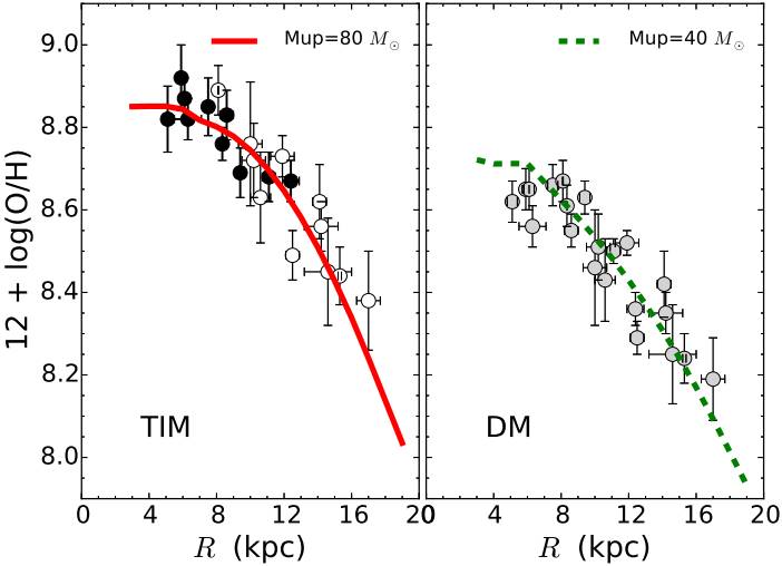
Fig. 1 Values of O/H as a function of the distance to the galactic
center. Models for t
2 = 0.00 and for observed
t
2 values versus two chemical evolution models with
different Mup
values. The filled and dashed lines represent the radial
distribution obtained with the TIM (
2.2. Representation of the Chemical Evolution Models
We compute a set of nine chemical evolution models (CEMs) for MW like galaxies based on the work by Carigi et al. (2019a); these models differ only in the adopted Mup value. We present the output of these models for 6.2 kpc, corresponding to the average galactocentric distance of M17 (6.1 kpc) and M8 (6.3 kpc), and for 8.34 kpc, corresponding to the galactocentric distance of the Orion Nebula.
The initial abundances of our models are: X(0) = 0.7549, Y (0) = 0.2451, C(0) = 0, and O(0) = 0, where Y (0) = 0.2451 ± 0.0026 is the primordial helium abundance derived by Valerdi et al. (2019). Their Y (0) result is in good agreement with the value derived by Planck Collaboration (2018) that amounts to Y (0) = 0.24687 ± 0.00076.
We explore the Mup effects on the predicted value of Y , C, and O during the whole evolution. The galaxies are formed in an inside-out scenario of primordial infall, with the halo component formed from 0 to 1 Gyr and the disk component formed from 1 to 13 Gyr.
In Figures 2 and 3 we present the ∆O vs ∆Y
evolution for R = 6.2 and 8.34 kpc,
respectively. Moreover, in Figures 4 and
5 we show ∆O vs
∆C evolution curves computed for the same radii. The
evolution curves are presented for nine CEMs that consider

Fig. 2 Chemical evolution for Y and O at a galactocentric distance of 6.2 kpc (approximatelly the distance of M17 and M8). The curves cover the entire evolution from the beginning (0 Gyr) to the present time (13 Gyr, magenta points), and each curve corresponds to a model with a different Mup . The squares represent the O and He abundances derived for M17 using the DM (grey) and the TIM (black); the diamonds represent the abundances derived for M8 using the DM (grey) and the TIM (black). The dotted magenta line connects the present-time values predicted by the models. Note that, the observed values should be compared with this magenta line to choose the better Mup values. The color figure can be viewed online.
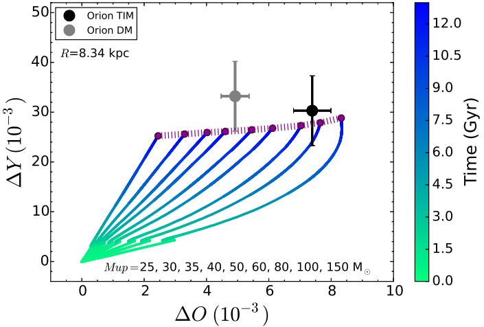
Fig. 3 Chemical evolution for Y and O at a galactocentric distance of 8.34 kpc (Orion). The curves cover the entire evolution from the beginning (0 Gyr) to the present time (13 Gyr, magenta points), and each curve corresponds to a model with a different Mup . The circles represent the O and He abundances derived for Orion using the DM (grey) and the TIM (black). Note that the Orion data should be compared with the magenta line (theoretical present-time values). The color figure can be viewed online.
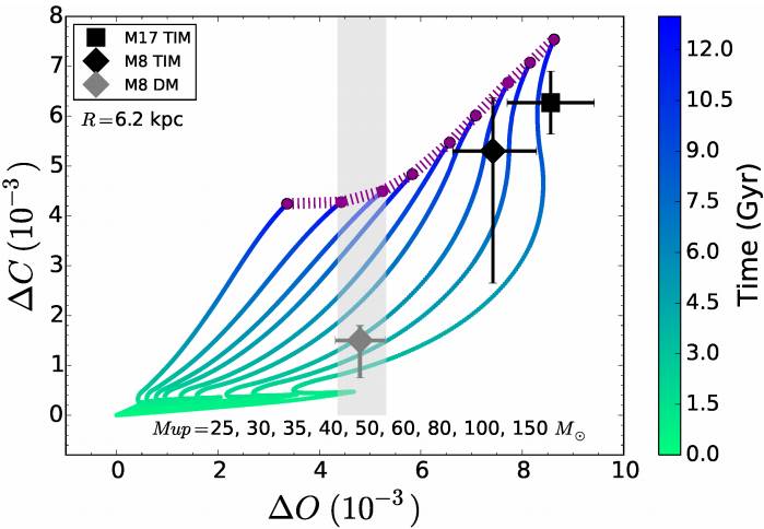
Fig. 4 Chemical evolution for C and O at a galactocentric distance of 6.2 kpc (approximately the distance of M17 and M8). The curves and points are similar to those in Figure 2. Notice, however, that there are only 3 points in this figure instead of the 4 in Figure 2: unfortunately there is no restriction on C for the DM of M17 and, instead of the fourth point the shaded vertical band is the ∆O predicted by the DM. Again, the observed values should be compared with the magenta curve. The color figure can be viewed online.
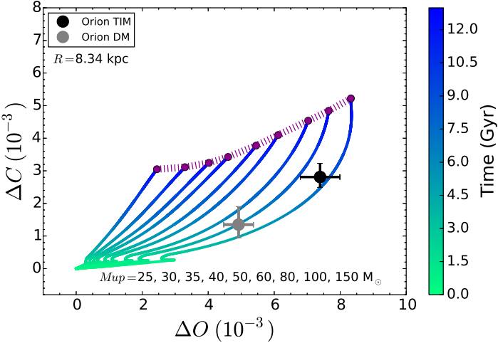
Fig. 5 Chemical evolution for C and O for a galactocentric distance of 8.34 kpc (Orion). The curves and points are similar to those in Figure 3. The Orion data should be compared with the magenta line. The color figure can be viewed online.
In Carigi et al. (2019a), models were built
to reproduce the radial behavior of the total O/H from 21H II regions. To fit a
representative absolute value of the gradient, they inferred two
Mup
values: one if the gaseous O/H values were determined from the DM
(
Also, for NGC 6822 (an irregular galaxy), Hernández-Martínez et al. (2011) built chemical evolution models to
reproduce O/H values determined from DM and TIM, and obtained
In this work, we will obtain uncertainty bars for the Mup values, comparing the present-time abundances computed by models using different Mup values, with the O/H, He/H, and C/H abundances (and their error bars) for M17, M8, and Orion.
2.3. Object Selection
The approach in this study is to put quality over quantity; thus, we only use three objects: the Orion Nebula, M17, and M8, since they are the most studied Galactic H II regions. One very important characteristic of the Orion Nebula and M17 is that they are very bright (hence their many studies); as a consequence of this they have arguably the best O/H abundance ratio determinations. Another reason to select them is that they have noticeable different galactocentric radii. While the Orion Nebula is, by far, the best studied H II region, M17 has the advantage of being a high ionization H II region and thus we do not need to worry about an uncertain ICF(He). Unfortunately, there are no UV observations of M17 (probably due to its relatively high c(Hβ) = 1.17) and it is therefore not possible to derive C abundances using CELs and the direct method. We selected M8 because it is also nearby and very bright, its galactocentric distance is very similar to that of M17 (allowing us to present both of them using the same simulation and figures), it is the 4th most observed Galactic H II region, and probably the 3rd best suited for a study such as the one we present.
Tables 1, 2, and 3 show the total abundances (gas + dust) by mass derived for M17, M8, and Orion, respectively. The values were derived by transforming the abundances by number obtained by García-Rojas et al. (2007); Esteban et al. (2005) for O/H, He/H, and C/H and assuming that O is approximately 45% of Z. The first column of these tables shows the abundances derived through the DM (from CELs) and assumes a constant temperature over the observed volume, whereas the second column shows the abundances derived through the TIM (from RLs).
TABLE 1 M17: OBSERVED ∆Y , O, AND C VALUESa
| DM | TIM | |
|---|---|---|
| ∆Y (10−3) | 37.7±4.2 | 30.1±4.1 |
| O(10−3) | 4.81±0.48 | 8.56±0.86 |
| C (10−3) | ... | 6.27±0.63 |
| ∆Y/∆O | 7.86±1.39 | 3.52±0.72 |
| ∆C/∆O | ... | 0.73±0.10 |
aObservations from García-Rojas et al. (2007).
TABLE 2 M8: OBSERVED ∆Y , O, AND C VALUESa
| DM | TIM | |
|---|---|---|
| ∆Y (10−3) | 42.2±8.5 | 22.1±7.8 |
| O(10−3) | 4.80±0.49 | 7.42±0.79 |
| C (10−3) | 1.50+0−0..3075 | 5.30+1−2..0765 |
| ∆Y/∆O | 8.80±1.99 | 2.84±1.06 |
| ∆C/∆O | 0.31+0−0..0716 | 0.68+0−0..1535 |
aObservations from García-Rojas et al. (2007).
TABLE 3 ORION NEBULA: OBSERVED ∆Y , O, AND C VALUESa
| DM | TIM | |
|---|---|---|
| ∆Y (10−3) | 33.2±7.1 | 30.3±7.0 |
| O(10−3) | 4.92±0.45 | 7.39±0.60 |
| C (10−3) | 1.35+0−0..5540 | 2.81+0−0..4232 |
| ∆Y/∆O | 6.75±1.45 | 4.10±1.01 |
| ∆C/∆O | 0.27+0−0..1208 | 0.38+0−0..0605 |
aObservations from Esteban et al. (2005).
As mentioned above, the line of sight in the direction of M17 has a relatively high reddening, and the λλ 1906-1909 Å ENT#091;C IIIENT#093; lines are too obscured to have been observed. One might be interested in using the λ 4267 Å C II line to complete the DM determination; but λ 4267 Å C II cannot be used as part as the DM for the same reasons that the λ 4650 Å O II multiplet cannot be used (since it corresponds to the TIM). Therefore, while widely used, it should not be considered as part of the DM (and one should beware of authors that use it as part of the DM without a clear and consistent explanation on the ADF origin and its consequences).
2.4. O/H vs. He/H
Gaseous O/H abundances are readily available from many observational sources. However, they are frequently not converted to the total ISM O/H; to do this, it is necessary to include the fraction of O trapped in dust grains. It is estimated that this correction is between 0.07 and 0.13 dex for most H II regions (Mesa Delgado et al. 2009; Peimbert & Peimbert 2010; Espíritu et al. 2017); the exact value depends on the metallicity and on the efficiency of the dust destruction present within each H II region. Here we will include a correction of 0.12 dex for the Orion Nebula (Mesa Delgado et al. 2009; Espíritu et al. 2017) and 0.11 dex for both M17 and M8(Peimbert & Peimbert 2010).
The C/H abundance should also be corrected for dust depletion; this correction is expected to be similar or slightly smaller than the O/H correction (Esteban et al. 1998, 2009). Here we will assume a correction of 0.10 dex for all three H II regions.
Although most elements should include a correction due to dust depletion, the fact that He is an inert noble gas means that no correction will be necessary for the He/H abundances.
2.4.1. O vs. Y for M17 and M8
In Figure 2 we present the theoretical evolution of ∆O and ∆Y vs time, for R = 6.2 kpc. We plot nine curves that correspond to the nine Mup values listed in § 2.2. The curves begin at t = 0Gyr (∆O = ∆Y = 0) and end at 13 Gyr. We include the ∆O and ∆Y values for M17 and M8, determined from the DM and the TIM (see Tables 1 and 2). In order to choose the Mup values that best reproduce the observational data, the top of each curve (the predicted values at present time (shown in magenta points) should be compared with the M17 and M8 data (the observed abundances for the ISM).
The curves evolve more rapidly to the right with increasing Mup values, because the O production for high mass stars (HMS) increases with the stellar mass. At 1 Gyr, when the halo formation ends, the curves present a loop due to the dilution of the ISM with primordial infall (Y = 0.2451, O = 0.0 Valerdi et al. 2019) that forms the disk. The rest of the evolution depends on the lifetime and the initial metallicity (Z) of the HMS and low-and-intermediate mass stars (LIMS), see Carigi & Peimbert (2008) and Carigi & Peimbert (2011) .
Current Y values are almost constant for
TABLE 4 PRESENT DAY VALUES IN THE ISM PREDICTED BY THE MODELS FOR R = 6.2 KPC (M17 AND M8)
| Mup | ∆Y (10 −3 ) | O(10 −3 ) | C(10 −3 ) | ∆Y/∆O | ∆Y/∆C |
|---|---|---|---|---|---|
| 150 | 39.16 | 8.63 | 7.54 | 4.54 | 1.14 |
| 100 | 37.14 | 8.15 | 7.08 | 4.56 | 1.15 |
| 80 | 35.92 | 7.72 | 6.67 | 4.65 | 1.16 |
| 60 | 34.79 | 7.08 | 6.01 | 4.91 | 1.18 |
| 50 | 34.40 | 6.57 | 5.47 | 5.24 | 1.20 |
| 40 | 34.18 | 5.83 | 4.86 | 5.86 | 1.20 |
| 35 | 34.09 | 5.24 | 4.50 | 6.51 | 1.16 |
| 30 | 34.19 | 4.43 | 4.28 | 7.72 | 1.04 |
| 25 | 34.19 | 3.36 | 4.24 | 8.06 | 0.79 |
A peculiarity of Figure 2 is the shape
of the
When comparing the observed O and He values for M17 with those derived from
our models we find: (i) for the ∆O value determined with
the DM, an IMF with a galactic Mup
of 30 - 36 M, while (ii) for the ∆O
value determined with the TIM, an
From the M8 values we find: (i) the ∆O value determined with
the DM is nearly identical to the one determined for M17; therefore, the
range determined for Mup
is also of 30 - 36
2.4.2. O vs. Y for the Orion Nebula
In Figure 3 we present curves of the theoretical evolution of ∆O and ∆Y vs time for R = 8.34 kpc, corresponding to nine Mup values listed in § 2.2. Moreover, we include the ∆O and ∆Y values for Orion, determined from the DM and the TIM (see Table 3). As in Figure 2, the top of each curve (in magenta) corresponds to the end of evolution (i.e. the present time; see Columns 2 and 3 of Table 5), and should be compared with the Orion data to choose the Mup values that best reproduce the observations.
TABLE 5 PRESENT DAY VALUES IN THE ISM PREDICTED BY THE MODELS FOR R = 8.34 KPC (ORION NEBULA)
| Mup | ∆Y (10 −3 ) | O(10 −3 ) | C(10 −3 ) | ∆Y/∆O | ∆Y/∆C |
|---|---|---|---|---|---|
| 150 | 28.82 | 8.32 | 5.22 | 3.46 | 5.52 |
| 100 | 27.87 | 7.65 | 4.84 | 3.64 | 5.76 |
| 80 | 27.30 | 7.03 | 4.54 | 3.88 | 6.01 |
| 60 | 26.77 | 6.12 | 4.10 | 4.37 | 6.53 |
| 50 | 26.45 | 5.45 | 3.77 | 4.85 | 7.02 |
| 40 | 26.12 | 4.60 | 3.42 | 5.68 | 7.64 |
| 35 | 25.91 | 4.02 | 3.24 | 6.45 | 8.00 |
| 30 | 25.50 | 3.30 | 3.11 | 7.73 | 8.20 |
| 25 | 25.24 | 2.45 | 3.04 | 10.30 | 8.30 |
In Figure 3, for any given Mup , the evolutionary curves reach lower ∆O and ∆Y values than the corresponding coeval values in Figure 2, because the O/H gradient is negative for all MW-like models. Therefore, for any given time, the ∆O value (and Z value) for R = 8.34 kpc is lower than the ∆O value for R = 6.2 kpc. Consequently, very few massive stars of high Z form and, since they are more efficient He producers, the reached Y values are lower. In this figure, for the Mup = 150 curve, the O dilution is lower, due to the relative lack of massive stars of high Z (highly-efficient C producers).
When comparing the observed O and He values for Orion with those derived from
our models, we find: (i) for the ∆O value determined with
the DM, an Mup
of 38 - 50 M; (ii) for the ∆O value
determined with the TIM, an
2.5. O vs. C
2.5.1. O vs. C for M17 and M8
In Figure 4 we show the curves of theoretical evolution of ∆O and ∆C vs time, for R = 6.2 kpc, obtained from our nine CEMs. The current values, at the top end of the curves, are presented in Columns 3 and 4 of Table 4. We include the observed ∆O and ∆C values for M17 and M8 determined from the TIM. The gray diamond represents the ∆O and ∆C values determined for M8, while the shaded vertical bar represents the ∆O for M17 using the DM combined with the lack of a C determination available from the DM (see Table 1).
A remark on the ∆C determination for M8: according to the recent ICFs computed for giant H II regions (Amayo, Delgado-Inglada, Stasińska, 2020, in prep.), the use of C/O = C++/O++ in M8 may underestimate the real C/O value by up to ≈ 0.3 dex. However, these ICFs may not be adequate for Galactic H II regions where only a small area is observed. We decided not to change the value of C/H but to increase the associated error bars.
Current C values are almost constant for
When comparing the observed ∆C value for M17 determined with
the TIM with those derived from the CEMs, we find an
Mup
in the 55 - 95 M range. Using the determination from
the M8’s ∆C measurements obtained with the TIM, we only
find an upper limit
2.5.2. O vs. C for Orion
In Figure 5 we show the theoretical evolution of ∆O and ∆C vs time for R = 8.34 kpc, for each of our nine Mup values. Moreover, we include the ∆O and ∆C values for Orion, determined from the DM and the TIM (see Table 3). In this figure, for any given Mup , the evolutionary curves reach lower O and C values than the coeval values in Figure 4, because the O/H and C/H gradients are negative for all the MW-like models.
By comparing the observed C values for Orion with the current values derived
from our models (see Table 5), we
find that neither set of observed ∆C abundances (neither DM
nor TIM) are consistent with the theoretical predictions. Since the
∆O values and determinations are the same as those in
Figure 3 it seems that the C
abundance in Orion is lower than expected; however, the C/H abundance in the
Orion nebula is noticeable smaller (about 0.1 dex) than in NGC 3603
(R = 8.65kpc) and NGC 3576
(R = 7.46kpc), which are the two H II
regions with a galactocentric distance closest to the one of the Orion
nebula (Esteban et al. 2004; García-Rojas et al. 2004; García-Rojas et al. 2006). There are
two causes that may explain this low value. The first one is the use of an
inadequate ionization correction factor (ICF); but according to a recent
study on ICFs for giant H II regions (Amayo et al. (2020) in prep.) it is
adequate to use C/O = C++/O++ to compute C abundances.
The second one is the possibility of this nebula having more C atoms
deposited in dust grains and thus, a lower gaseous abundance of C; a clue
that the dust properties in Orion are different than in other H II regions
is the high total to selective absorption ratio present in Orion, that
amounts to about RV
= EV
/EB−V
≈ 5.5 (Peimbert
& Costero 1969; Esteban et
al. 2004), while for most other objects it amounts to about
RV
= 3.1 (Cardelli et
al. 1989). If we consider that Orion could have a slightly higher
(0.1 dex) total C abundance, we find, for the TIM, the total gas plus dust
ratio of C/H for the Orion nebula to be 12 + log(C/H) ≈
8.53 ± 0.08; this value represents a
slightly lower Mup
than the one derived from O/H. On the other hand, we find, for the
DM, the total C/H to be 12+log(C/H) ≈
8.22±0.10, still 0.1 dex less than our
lowest model, approximately 0.2 dex lower than the
3. THE CHEMISTRY HAS A BETTER MEMORY THAN THE LIGHT
The lifetime of massive stars (few Myr) is very short compared to the age of galaxies (several Gyr); consequently, massive stars are not an important component of the light of the majority of the observed galaxies; yet, when massive stars die, their contributions are quickly incorporated into the chemistry of the ISM.
The chemical composition of an H II region is the result of the whole history of the chemical evolution of any given galaxy; therefore the chemical composition of H II regions can be compared with estimates of the present day chemistry derived from galactic CEMs; and we can infer the amount of formed massive stars (equivalently, the Mup value), comparing the chemical abundances in the ISM with those obtained from CEMs.
To study the most massive stars in the MW by looking for them at present has several major inconveniences: there are very few of these stars, this is compounded by the fact that they must be formed in very massive giant molecular clouds (GMCs), and they are the first ones to evolve (first shedding mass in strong stellar winds, and then going supernova, all this before the GMC is dissipated by the combined effect of the stars that are evolving inside it). Thus, they are usually obscured and very difficult to observe during their short lifespan. Moreover, most massive stars that can be observed today may not be representative of the most massive stars that have existed during the evolution of the Galaxy, i.e. the stars that have contributed to the evolution of the chemistry of the present day ISM as well as the chemistry available during the most recent star formation.
Based on the ∆Y comparison, between the observed values (from TIM or
DM) and the preset-time predicted values (from CEMs), we cannot exclude any
Mup
value in the 25 - 150
Weidner et al. (2013) in their Figure 3 showed the dependence of the star
formation rate (SFR) on the integrated galactic stellar initial mass function
(IGIMF, called IMF in our CEMs) for different power-law indexes, α,
(for initial stellar masses between 1.3 M and
Mup
). They noted that IMF for a SFR
Regarding the observational determinations of the SFR: (i) the MW, a spiral galaxy
(Sbc) with total stellar mass
Moreover, based on spatially-resolved spectroscopic properties of low-redshift
star-forming galaxies, Sánchez (2019) showed
in his Figure 7 a difference of approximately 1 order of magnitude between the SFR
of Sbc galaxies with stellar mass ≈ 1011
M (as the MW galaxy) and the SFR of Sd galaxies with stellar mass
Therefore, the Mup values we derive from the TIM are consistent with the SFR of the MW galaxy, while the Mup values derived from the DM are consistent with a galaxy with a mass and SFR similar to those of NGC 300, but not with the mass and SFR of the MW.
Moreover the abundances derived from the TIM are consistent with those derived from observation of other young objects in the MW (Cepheids, B stars), while the abundances derived from the DM are approximately 0.25 dex too small.
The chemical composition of a given H II region is the result of the evolution of the ISM throughout the history of our Galaxy. Therefore, the chemical abundances of an H II region do not depend on the IMF of the observed H II region. In particular the most massive star of a given H II region is not representative of the most massive stars of the galactic IMF.
4. CONCLUSIONS
We have computed nine chemical evolution models (CEM) of a MW like galaxy; the only
difference among these models is the IMF, specifically its M
up value, that ranges between 25 and 150
It is useful to remember that the chemistry has a better memory than the observed UV light. In other words: the chemistry will explore the average Mup over the lifespan of the MW, while any measurement of the UV radiation or of the most massive stars observed can only be a reflection of the present day Mup (and can potentially have significant biases toward lower masses).
When comparing the models with the DM abundances we find: for ∆O, a
Moreover the Mup
in a given galaxy is directly related to the SFR, and the SFR is directly
related to the mass of any given galaxy. A MW like galaxy, with a SFR

