


 nova página do texto(beta)
 Inglês (pdf)
 Artigo em XML
 Referências do artigo
 Enviar este artigo por email
 Citado por SciELO
  Similares em
SciELO
Similares em
SciELO 
 Permalink
1.Introduction
Although late-type galaxies are relatively simple systems and are the most abundant galaxies in the Universe (Marzke & Da Costa, 1997; Mateo, 1998; Danieli, S. et al. 2017), their formation and evolution are not yet well understood. Although there are many different parameters which might influence the evolution of galaxies, one of the most important is the star formation rate (SFR). The reasons are many. The SFR indicates how many stars are formed by the gas in a galaxy (in time). Therefore, gas mass is transformed into stars, which then process this gas transforming the primordial hydrogen into more complex atoms, like oxygen, sulfur, or iron (see, for example, the seminal work of Tinsley on chemical evolution; Tinsley 1981). Moreover, massive stars end their lives as supernovae, which inject about 1051erg of energy into the interstellar medium (ISM) of the galaxy (Pittard, 2019). Such energy can be used to collapse the gas in the vicinity and form new stars (as in Holmberg II or IC 2574, Sánchez-Salcedo, 2002), to heat the medium avoiding a new event of star formation (Jog, 2013), or even to eject gas (and metals) outside the galaxy (e.g. Dekel & Silk, 1986; D’Ercole & Brighenti, 1999; Melioli et al. 2015). In order to have a wider and more comprehensive view of such events, other parameters are needed, such as the initial mass function (IMF) which gives the number of stars formed for each mass interval, and the star formation history (SFH), which is the number of stars formed along cosmic time in each galaxy. This set of parameters (SFR, IMF and SFH) provide information about the evolution of galaxies (López et al. 2018).
The SFR can be determined by several diagnostic methods. Two of the most important are the intensity of the recombination line Hα and the flux of the FUV (Kennicutt, 1998; Calzetti 2013; Audcent-Ross et al 2018). The Hα line has been widely used due to its many advantages, such as being easy to measure even with small aperture telescopes, because of its large flux in star-forming galaxies. Nevertheless, for galaxies with z > 0.5, the Hα line goes into the near infrared and it is necessary to use a detector in this wavelength range. The UV measurements also allow the determination of the SFR from the FUV continuum. Several authors have noticed differences in the SFR obtained from the Hα line and the FUV continuum and have given possible explanations for the discrepancies (e.g. Bell & Kennicutt, 2001; Lee et al. 2009): an IMF systematically deficient in the highest mass stars, a leakage of ionizing photons from a low density environment, or the fact that most methods only consider a single, solar metallicity. Most of these studies have been done on spiral and irregular galaxies of the local volume and for dwarf galaxies within 11 Mpc (Karachentsev & Kaisina, 2013; Lee et al. 2009).
It is well known that the highest star formation rates occur in Sc galaxies (Kennicutt, 1998). Late-type galaxies (Sm and dS) have a very large reservoir of neutral gas relative to their total mass (typically of the order of 6%, Huchtmeier & Richter, 1989) but a lower SFR (e.g. Hunter & Elmegreen, 2004). Therefore, the efficiency of the star formation process is very low for these galaxies. There could be several reasons for this; the lack of a clear triggering mechanism of star formation could be one of the most important ones.
There are several goals in this paper, which is focused on the integrated SFR values of a sample of late-type galaxies. Firstly, to increase the sample of late-type galaxies with SFR measurements based on Hα and FUV flux. Although there are many investigations devoted to SFR determinations (among others, James et al. 2004; Lee et al. 2009; Hunter & Elmegreen 2004; Hunter et al., 2010; Rosenberg et al. 2008; Buat et al. 2009; Boselli et al. 2015; Boselli et al. 2009; James et al. 2008; Almoznino & Brosch, 1996) there are only 50 Sm galaxies with SFR determined from the FUV continuum, so the inclusion of another 28 galaxies increases the total sample by more than 50%. The increase is not so large for Sm galaxies with SFR based on the recombination line Hα: only about 15%.
Another goal is to check how much dS galaxies differ from Sm galaxies. Among other things, we can check the efficiency of the SFR, because dS galaxies have a larger amount of neutral gas but a less clear spiral structure, as stated above.
Another interesting study performed here is the spatial distribution of the HII regions in the galaxies. Some authors claim that most of the regions are located in the central part of the galaxies (e.g Roye & Hunter, 2000; Hodge, 1969; Bruch et al. 1998), and that, for barred galaxies, many HII regions are located at the end of the bar (Elmegreen & Elmegreen, 1980). This is tested for the galaxies in our sample. Moreover, if there is any large asymmetry in the HII region distribution, some clues on the recent environmental history can be obtained.
Finally, we want to study how the diffuse ionized gas (hereafter, DIG) might affect the estimation of the SFR in galaxies, because not all the Hα emission outside the HII regions is due to ionizing photons emitted by massive stars, but also to mechanisms (See Hidalgo-Gámez 2004 for a review). So, the inclusion of DIG photons in the total Hα emission might give a higher, but not so accurate, SFR.
The paper is organized as follows. In § 2 we describe the galaxy sample, the data acquisition, reduction and calibration of data as well as the detection of the Hii regions. The determination of the SFR values with the Hα and FUV fluxes, along with a contrast of our results with the data from the literature, and the efficiency of the star formation process are studied in § 3, while the results on the distribution of the HII regions in our sample are outlined in § 4. Finally, the importance of the DIG on the estimation of the SFR is discussed in § 5. Our conclusions are presented in § 6.
2.Sample Description, Data Acquisition and Reduction
The sample used in this investigation consists of 36 late-type galaxies, that are divided into 14 dwarf spiral galaxies (dS) and 22 Sm galaxies. The galaxies in the latter subsample were selected from the RC3 and UGC catalogues, considering only Sm or types 9 or 10 galaxies. The galaxies in the former subsample were selected from Table 1 in Hidalgo-Gámez (2004). All interacting and active galaxies were disregarded. Ten of the galaxies in this sample are classified as barred, 7 of them are Sm and 3 dS. Finally, from a visual inspection of the Hα images we divided our sample into galaxies with clear spiral structure (18 galaxies), galaxies without spiral structure (9 galaxies) and those of intermediate type (9 galaxies). The galaxies in the sample presented here were selected from the tables mentioned above and observed just because their coordinates were the right ones at the moment of the observations.
Table 1 Global Parameters
| Galaxy - | Type | α 2000 | δ 2000 | MB [mag] | r25 [kpc] | D [Mpc] | AR [Mag] | i [o] | μB [mag/arcsec2] | M(HI) [Mʘ*109] | ∑HI[Mʘpc2] | log(MHI/LB) |
| DDO 18 | Sm | 02 10 44 | 06 45 30 | -18.37 | 6.59 | 20.70 | 0.13 | 70 | 23.8 | 0.99 | 5.57 | -1.72 |
| UGC 560 | Sm | 00 54 47 | 13 39 29 | -20.5 | 10.57 | 72.70 | 0.21 | 24 | 26.1 | - | - | - |
| UGC 3086 | Sm | 04 32 55 | 00 32 12 | -16.64 | 9.75 | 73.50 | 0.18 | - | - | 4.61 | 12.85 | -1.45 |
| UGC 3778 | Sm | 07 16 55 | 28 31 46 | -17.97 | 9.57 | 65.80 | 0.14 | - | - | 4.1 | 11.44 | -1.94 |
| UGC 3947 | Sm | 07 39 02 | 33 54 59 | -17.12 | 7.41 | 55.90 | 0.10 | 45 | 24.7 | 1.35 | 9.20 | -1.94 |
| UGC 3989 | Sm | 07 44 41 | 53 50 05 | -17.76 | 11.56 | 79.50 | 0.11 | 0 | 26.3 | - | 9.21 | - |
| UGC 4121 | Sm | 07 58 54 | 54 02 33 | -17.55 | 6.44 | 18.90 | 0.08 | 72 | 24.3 | 1.2 | 6.69 | -1.23 |
| UGC 4797 | Sm | 09 08 11 | 05 55 40 | -17.41 | 5.43 | 19.60 | 0.10 | 24 | 24.2 | 0.62 | - | -1.5 |
| UGC 4837 | Sm | 09 21 10 | 35 31 54 | -17.50 | 8.78 | 28.90 | 0.06 | 51 | 24.5 | 1.84 | 14.46 | -1.4 |
| UGC 5236 | Sm | 09 47 00 | 21 43 47 | -20.54 | 10.00 | 53.40 | 0.08 | 12 | 25.3 | 0.03 | 0.09 | -4.92 |
| UGC 6151 | Sm | 11 05 56 | 11 49 35 | -17.29 | 6.73 | 24.30 | 0.06 | 45 | 24.3 | 0.88 | 4.74 | -1.47 |
| UGC 6205 | Sm | 11 09 59 | 46 05 44 | -19.58 | 4.99 | 27.30 | 0.04 | 41 | 23.7 | 0.31 | 3.96 | -2.94 |
| UCG 6399 | Sm | 11 23 23 | 50 53 34 | -18.02 | 8.13 | 20.30 | 0.04 | 74 | 23.1 | 0.69 | 7.36 | -1.71 |
| UCG | 8253 | Sm | 13 10 44 | 11 42 28 | -17.72 | 11.16 | 53.10 | 0.07 | 17 | 25.4 | - | -1.82 |
| DDO | SBm | 05 07 47 | -16 17 37 | -18.74 | 8.49 | 24.90 | 0.17 | 54 | 23.1 | - | - | - |
| NGC 2552 | Sm | 08 19 20 | 50 00 35 | -19.37 | 5.14 | 10.20 | 0.12 | 49 | 23.5 | 0.74 | 8.62 | -1.63 |
| NGC 4010 | SBm | 11 58 38 | 47 15 41 | -20.47 | 11.29 | 18.20 | 0.05 | 79 | 22.9 | 2.57 | 16.1 | -2.0 |
| UGC 4871 | SBm | 09 14 57 | 39 15 45 | -17.79 | 9.14 | 37.00 | 0.03 | 69 | 23.7 | - | 6.18 | - |
| UGC 83 85 | SBm | 13 20 38 | 09 47 14 | -19.70 | 7.29 | 22.40 | 0.05 | 56 | 23.7 | - | - | - |
| UGC 10058 | SBm | 15 50 24 | 25 55 21 | -17.99 | 5.49 | 34.4 | 0.14 | 42 | 25.3 | - | - | - |
| UGCA 117 | SBm | 06 00 35 | -28 59 31 | -19.53 | 11.50 | 30.75 | 0.08 | 56 | 23.0 | 1.4 | 11.86 | -2.37 |
| UGC 2345 | SBm | 02 51 53 | -01 10 20 | -16.23 | 7.16 | 14.20 | 0.19 | 29 | 27.0 | - | - | - |
| UCG 3775 | dS | 07 15 53 | 12 06 54 | -17.34 | 4.68 | 29.40 | 0.24 | 27 | 25.3 | 0.41 | 5.96 | -1.99 |
| UCG 4660 | dS | 08 54 24 | 34 33 22 | -15.96 | 5.57 | 32.60 | 0.06 | 21 | 25.5 | 1.5 | 8.52 | -0.96 |
| UGC 5296 | dS | 09 53 11 | 58 28 42 | -16.06 | 3.02 | 25.20 | 0.03 | 29 | 24.5 | 0.29 | 10.12 | -1.5 |
| UGC 5740 | dS | 10 34 46 | 50 46 06 | -16.63 | 2.86 | 11.30 | 0.05 | 46 | 24.6 | 0.41 | 6.31 | -0.87 |
| UCG 6304 | dS | 11 17 49 | 58 21 05 | -16.40 | 4.72 | 28.90 | 0.03 | 39 | 25.0 | - | - | - |
| UCG 6713 | dS | 11 44 25 | 48 50 07 | -16.68 | 3.66 | 17.00 | 0.05 | 44 | 24.0 | 0.9 | 13.78 | -0.9 |
| UGC 9018 | dS | 14 05 33 | 54 27 40 | -14.95 | 1.59 | 6.58 | 0.03 | 37 | 23.7 | 0.13 | 13.78 | -0.23 |
| UCG 9902 | dS | 15 34 33 | 15 08 00 | -15.93 | 3.67 | 27.70 | 0.13 | 72 | 23.5 | - | - | - |
| UCG 9570 | dS | 14 51 36 | 58 57 14 | -17.46 | - | 35.50 | 0.03 | - | - | - | - | - |
| UCG 11820 | dS | 21 49 28 | 14 13 52 | -15.79 | 4.96 | 17.10 | 0.33 | 24 | 25.5 | 1.54 | 19.96 | -0.32 |
| UCG 12212 | dS | 22 50 30 | 29 08 18 | -20.77 | 3.30 | 19.50 | 0.17 | 56 | 24.1 | 0.8 | 23.38 | -2.72 |
| UCG 891 | dSB | 01 21 19 | 12 24 43 | -17.30 | 3.13 | 9.40 | 0.08 | 63 | 24.1 | 0.36 | 11.70 | -1.04 |
| UCG 5242 | dSB | 09 47 06 | 00 57 51 | -20.57 | 4.86 | 26.30 | 0.34 | 50 | 24.0 | 0.8 | 10.78 | -2.9 |
| UCG 6840 | dSB | 11 52 07 | 52 06 29 | -16.99 | 4.60 | 17.00 | 0.06 | 72 | 22.9 | 1.04 | 12.77 | -0.97 |
The number of Sm galaxies studied here is comparable with other samples [ 8 Sm galaxies in James et al. (2004), 20 Sm in Hunter & Elmegreen (2004), 25 Sm in van Zee (2001) and 7 Sm galaxies in Hunter et al. (2010)].
The characteristics of the galaxies in the sample are presented in Table 1 The name and the morphological type is given in Columns 1 and 2, while the coordinates (α and δ) are listed in Columns 3 and 4 from NED-NASA. The absolute magnitude (Column 5) was determined from the apparent magnitude and the kinematic distance (Column 7) which were obtained from the NASA Extragalactic Database (NED-NASA). The absolute magnitudes are galactic extinction-corrected (Column 8). The inclination is presented in Column 9 and was also obtained from NED-NASA. The optical size (Column 6) and the surface brightness (Column 10) were determined following equations 3 and 4 in Hidalgo-Gámez & Olofsson (1998). Finally, the Hi mass and surface density were computed from equation 2 in Hidalgo-Gámez (2004).
2.1.Observations, Reduction and Calibration of the Data
The Hα images were acquired at the 1.5m telescope of the Observatorio Astronómico Nacional at San Pedro Mártir (OAN-SPM) in five different observational campaigns from 2002 to 2004. Five narrow band filters were used: three in the hydrogen Hα recombination line, centered at 6570 Å, 6607 Å and 6690 Å, and two for continuum subtraction, with central wavelengths at 6459 Å and 6570 Å. The maximum transmittance of the filter was 70% and they were between 89 Å and 127 Å wide. The integration times were in the range of 1200 and 5400s for hydrogen Hα and 900 and 3600s for continuum, respectively. The air mass was smaller than 1.4 for all but three of the galaxies, and the seeing was between 1.1 and 2.6, with an average value of 1.4. The convolution of the peak transmission of the filters (70%) and the high detector quantum efficiency (90%) allowed us to achieve relatively deep flux limits (7 x 10-18ergcm-2s-1).
The reduction procedure (bias, flat-fields, removal of cosmic rays and sky subtraction) as well as the flux calibration were performed using the ESO-MIDAS software. Three standard stars were observed each night with different air mass in order to perform the flux calibration.
The ultraviolet fluxes were obtained from the 6th release (GR6) of the GALEX database for a total of 30 out of the 36 galaxies of the sample. We used those data with an exposure time of 1500s. Both the FUV and NUV fluxes were determined for the 30 galaxies from the integrated flux provided by the conversion from AB magnitudes: Fv[erg s-1cm-2Hz-1] ECUACION. Full details of the telescope, instruments, calibration and processing pipeline are provided by Martin et al. (2005) and Morrissey et al. (2005, 2007).
2.2.HII Regions Detection
In order to obtain the SFR, fluxes from the Hα line are needed as well as from the FUV continuum. The simplest approach is to consider the galaxy emission as a whole, e.g. the continuum-subtracted Hα emission. However, as we were interested in a further analysis of the data (such as the luminosity function and the location of the HII regions inside the galaxies) we decided not to use that technique. Instead, we selected the HII regions from the continuum-subtracted Hα images. Only those regions identified by two of us were included in the sample. A circular aperture centered on each region was used to determine the flux. Two different radii were considered for each Hii region. The first one included all the emission of the region and the second one included only the emission with flux values larger than a limiting value, in order to distinguish between proper Hii regions and DIG. As will be discussed in § 6, this limiting flux has been determined by spectroscopic studies and is of 10-17erg s-1cm-2. This procedure was performed manually; the radius aperture just depends on the galaxy distance, which defines the size of the region in the image.
The main disadvantage of this procedure is the difficulty to detect very low luminosity regions. However, as they are very faint, the contribution of their fluxes to the SFR is not significant and will only be important in the study of the luminosity function of the Hii regions inside the galaxies.
In the case of galaxies with large inclinations, it is very difficult to
distinguish different regions if they are in the same line-of-sight. This is the
situation for 7 of the galaxies in our sample, which have inclinations larger
than 70. It can be argued that the inclusion of such galaxies in our sample is
not correct because of the difficulty of an accurate extinction correction.
However, most of the classical studies of the SFR in galaxies have included high
inclination objects without any further correction (e.g. James et al. 2008; Lee et
al. 2009; Hunter et al. 2010;
Boselli et al. 2015). In 2018, Wang et
al. studied the influence of the inclination on the SFR value and they concluded
that the inclination is important only for galaxies more massive than
A similar problem might appear for those Hii regions which are very close and cannot be separated due to the resolution of our observations.
With the knowledge of the positions of the Hii regions from the Hα images, the GALEX images were inspected to locate the star forming regions and the fluxes from these locations were calculated.
2.3.Flux Corrections
Before the SFR could be determined, the UV and Hα fluxes need to be corrected for extinction. There are contributions to the extinction (i) from the gas inside the galaxy (hereafter, the internal extinction), (ii) due to the intergalactic medium, (iii) due to gas inside our own Galaxy, and (iv) due to the atmosphere. The last one was corrected for the standard way. To correct for Galactic extinction we followed Cardelli et al. (1989), using values of RV from 2.6 to 5.5 (Clayton & Cardelli, 1988) and considering the color excess values from NED.
The most difficult extinction correction is the extinction internal to the galaxy. Since there is no simple way to estimate the extinction coefficient in Hα, A(Hα), this correction is not generally performed. In this article, the determination of the internal extinction coefficient for Hα was computed following Calzetti et al. (2000), where they derived an extinction law K(λ) directly from the data in the UV and optical wavelength ranges, as in Calzetti (1997b). As K(λ) is related to the internal nebular extinction, the extinction coefficient in Hα can be obtained as:
On the other hand, we followed the formalism of Salim et al (2007) to estimate the extinction coefficient in FUV,
where
The internal extinction increased the final fluxes in the galaxies of our sample 15% on average, but the increease was up to 50% for three of the galaxies (UGC 560, UGC 5242, UGC 12212).
Because of the large bandwidth of the filters used in this work (larger than 70 Å), the Hα flux is contaminated with the nitrogen line emission. From our own spectroscopy data of several of the galaxies presented here, the [NIII]/Ha ratio is typically smaller than 0.1 (Hidalgo-Gámez et al. 2012). The flux obtained from our images was then corrected by 10% in order to eliminate this contribution.
3.Integrated Star Formation Rates
The star formation rates were determined from the corrected Hα and FUV fluxes using the Kennicutt (1998) expressions. The total flux is the sum of the fluxes for all the Hii regions. Recently, Hunter et al. (2010) obtained a new SFR calibration for low metallicity galaxies. There are differences of about 15% in the SFR values determined with the Hunter or Kennicutt expressions. Although the galaxies in our sample have subsolar metallicity (Hidalgo-Gámez et al., in preparation; Hidalgo-Gámez et al. 2012) we used Kennicutt’s because the comparison with previous work is straightforward. The SFR values determined with Hunter et al.’s expressions are listed in Columns 7 (Hα) and 9 (UV) of Table :2 for a quick comparison with the Kennicutt values. The expressions used by Kennicutt (1998) are
The distance used to determine the luminosities is the so-called kinematic distance, D=V LG /H0, corrected by the Virgo Cluster infall, where Ho is 73 km s-1Mpc-1 (Riess et al. 2011).
The SFRs from Hα and FUV for all galaxies, separated by morphological type, as well as the total fluxes and the extinction values for both bands, are shown in Table 2. Two different fluxes were considered for Hα, with and without DIG. The latter values are shown in the last column of Table 2 (see § 6 for details). The errors were determined considering the uncertainties in the distance and the error associated with the flux determination.
Table 2 Hα and FUV star formation rate
| Galaxy | F Hα 10-4 [erg s-1]cm-2 | AHα [mag] | FFUV 10-28 [erg s-1 Hz-1] | AFUV [mag] | SFR(Hα)DIG [Mʘyr -1]10-2 | SFR(Hα)Hunter [Mʘyr -1]10-2 | SFR(FUV) [Mʘyr -1]10-2 | SFR(FUV)Hunter [Mʘyr -1]10-2 | SFR(Hα) [Mʘyr -1]10-2 |
| DDO 18 | 9.12 | 0.28 | 0.95 | 0.78 | 17±2 | 14.8 | 14± 2 | 12.70 | 3.7± 0.5 |
| UGC 560 | 11.13 | 0.77 | 0.10 | 2.11 | 113±17 | 97.78 | 63± 10 | 57.14 | 56 ± 8 |
| UGC 3086 | 19.10 | - | - | - | 109±5 | 95.2 | - | - | 97 ± 3 |
| UGC 3778 | 6.04 | - | - | - | 108 ± 16 | 94.28 | - | - | 25 ± 3 |
| UGC 3947 | 1.01 | - | - | - | 5.8±0.9 | 5.1 | - | - | 2.9± 0.6 |
| UGC 3989 | 1.23 | 0.19 | 0.43 | 0.52 | 66 ±2 | 57.6 | 74 ± 13 | 67.12 | 7.3± 0.4 |
| UGC 4121 | 1.19 | 0.25 | 0.55 | 0.69 | 3.7 ± 0.8 | 3.2 | 6.0 ± 1.0 | 5.44 | 0.4± 0.1 |
| UGC 4797 | 1.13 | 0.05 | 2.33 | 0.13 | 4.1±0.7 | 3.6 | 17 ± 2 | 15.42 | 0.41± 0.07 |
| UGC 4837 | 7.02 | 0.00 | 0.72 | 0.01 | 19±3 | 17 | 10 ± 4 | 9.07 | 5.5 ± 0.7 |
| UCG 5236 | 6.63 | 0.62 | 0.33 | 1.70 | 18±8 | 16 | 76±14 | 68.93 | 18±4 |
| UCG 6151 | 1.20 | 0.01 | 1.21 | 0.03 | 7.1 ±0.9 | 6.2 | 12±2 | 10.88 | 0.67±0.08 |
| UGC 6205 | 5.23 | 0.31 | 0.90 | 0.85 | 4±1 | 3 | 25±4 | 22.68 | 4±1 |
| UCG 6399 | 0.45 | 0.04 | 0.56 | 0.10 | 1.5±0.4 | 1.3 | 4±1 | 3.63 | 0.18±0.04 |
| UGC 8253 | 1.56 | 0.03 | 0.03 | 0.09 | 4.3±0.2 | 3.8 | 1.5±0.5 | 1.36 | 4.2±0.2 |
| DDO 36 | 21.94 | - | - | - | 69±10 | 60 | - | - | 13±2 |
| NGC 2552 | 103.89 | 0.34 | 9.72 | 0.92 | 15±4 | 13 | 39±4 | 35.37 | 10±3 |
| NGC 4010 | 1.50 | 0.42 | 1.30 | 1.16 | 5.8±0.6 | 5.1 | 21±6 | 19.05 | 0.47±0.07 |
| UGC 4871 | 1.39 | 0.00 | 0.61 | 0.01 | 15.4±0.4 | 13.4 | 14±2 | 12.69 | 1.80±0.05 |
| UCG 8385 | 8.03 | 0.39 | 2.03 | 1.07 | 6.0±0.3 | 5.2 | 45.7 | 41.45 | 3.8±0.3 |
| UGC 10058 | 0.07 | 0.60 | 0.22 | 0.08 | 1.5±0.3 | 1.3 | 3.7±0.5 | 3.36 | 2.5±0.5 |
| UGCA 117 | 0.54 | 0.01 | 1.91 | 0.04 | 4.9±0.7 | 4.3 | 31±5 | 28.12 | 0.49±0.06 |
| UGC 2345 | 29.73 | 0.27 | 5.03 | 0.73 | 12±1 | 10 | 33±4 | 29.9 | 5.7±0.6 |
| UCG 3775 | 2.88 | 0.16 | 0.69 | 0.45 | 6±1 | 5 | 15±2 | 13.6 | 2.3±0.9 |
| UGC 4660 | 4.24 | - | - | - | 6±1 | 5 | - | - | 4.3±0.6 |
| UGC 5296 | 2.56 | - | - | - | 2.3±0.2 | 2.0 | - | - | 1.5±0.1 |
| UGC 5740 | 4.05 | 0.31 | 1.57 | 0.86 | 2.1±0.3 | 1.8 | 7±1 | 6.35 | 0.49±0.06 |
| UGC 6304 | 3.74 | 0.01 | 2.06 | 0.04 | 5.6±0.1 | 4.9 | 30±4 | 27.21 | 2.95±0.07 |
| UGC 6713 | 4.47 | 0.09 | 1.65 | 0.25 | 1.3±0.3 | 1.1 | 10±4 | 9.07 | 1.2±0.3 |
| UGC 9018 | 7.72 | 0.02 | 5.52 | 0.05 | 1.0±0.1 | 0.9 | 4.2±0.6 | 3.81 | 0.32±0.04 |
| UGC 9902 | 0.00 | 0.01 | 0.13 | 0.02 | 0.00 | 0.00 | 1.7±0.3 | 1.54 | 0.00 |
| UGC 9570 | 0.19 | 0.15 | 1.52 | 0.40 | 2.3±0.1 | 2.0 | 46±6 | 41.72 | 0.23±0.01 |
| UGC 11820 | 5.30 | 0.02 | 0.46 | 0.05 | 1.7±0.4 | 1.5 | 2.3 | 2.09 | 1.5±0.3 |
| UGC 12212 | 20.23 | 0.91 | 0.67 | 2.50 | 14±2 | 12 | 42±6 | 38.1 | 7.3±0.9 |
| UGC 891 | 8.27 | 0.41 | 2.51 | 1.12 | 2.6±0.4 | 2.3 | 10±1 | 9.07 | 0.70±0.3 |
| UGC 5242 | 2.97 | 0.76 | 0.24 | 2.07 | 6.0±0.8 | 5.2 | 19±3 | 17.23 | 1.9±0.2 |
| UGC 6840 | 2.79 | 0.01 | 0.74 | 0.02 | 2.01±0.02 | 1.75 | 4±2 | 3.63 | 0.76±0.02 |
3.1.Star Formation Rates of Late-Type Galaxies from Hα Luminosities
From a closer inspection of Column 6 in Table 2, it can be concluded that there are three ranges in the SFR (Hα) values: galaxies with values larger than 1Mʘyr-1 (3 galaxies), those with SFR(Hα) between 0.1 and 1Mʘyr-1 (9 galaxies), and galaxies with values smaller than 0.1Mʘyr-1 (24 galaxies). For the galaxy UGC 9902 the SFR is taken as zero because we could not detect any Hα flux in it. The distribution of the SFR(Hα) values for all the galaxies in the sample is shown in Figure 1 (left). The distribution is not symmetrical, showing a clear asymmetry towards the low SFR values.
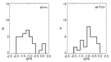
Fig. 1 Star formation rate distributions for all the galaxies in the sample from Hα fluxes with DIG (left) and from FUV continuum (right). The range comprised for the Hα fluxes is wider than for the FUV, with the bulk of galaxies having SFR below 0.1 Mʘyr-1 for the former and between 1 and 0.1 for the latter
The galaxy with the largest SFR(Hα) value is UGC 560, one of the most distant in our sample, with a SFR similar to that of the Milky Way (MW) (1.7 Mʘyr-1, Robitaille & Whitney, 2010) while the one with the smallest SFR is UGC 9018, a dS galaxy which is the nearest, one of the smallest in size, and with very few gas left.
As can be seen from Figure 2 (left plots), where the distribution for Sm galaxies is shown in the top row while the one for dS galaxies in the bottom row, the former have larger SFR values than the dS galaxies: a factor of 4.7, according to the average values shown in Table 3 (second column). Actually, only one out of 14 dS galaxies has a SFR larger than 0.1 Mʘyr-1. One explanation might be the small number of dS galaxies in our sample. However, they are almost a 40% of the total sample and, therefore, such differences might be due to another reason. We will further discuss this in § 3.6.
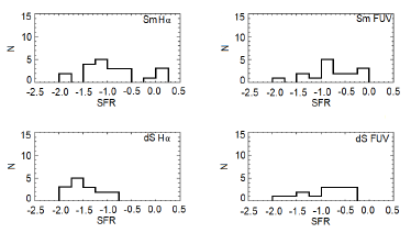
Fig. 2 Star formation rate distribution for the Sm galaxies (upper row) and dS galaxies (bottom row). The left plots show the values from the H α line (SFR(H α ) DIG ); the values from the FUV are plotted on the right.
Table 3 Averaged star formation rate
| Hα | σ | Without DUG | σ | FUV | σ | |
|
All All Sm All dS |
0.19 0.28 0.06 |
0.2 0.4 0.05 |
0.08 0.12 0.02 |
0.03 0.2 0.03 |
0.23 0.27 0.16 |
0.3 0.4 0.2 |
|
Borred Sm Non-barred Sm |
0.12 0.22 |
0.02 0.04 |
0.03 0.10 |
0.2 0.4 |
0.20 0.24 |
0.5 0.2 |
| Barred Sm Non-barred Sm Barred dS Non-barred dS |
0.17 0.33 0.03 0.04 |
0.02 0.04 0.03 0.05 |
0.04 0.16 0.01 0.02 |
0.05 0.03 0.01 0.4 |
0.25 0.28 0.11 0.18 |
0.6 0.3 0.2 0.2 |
Averaged star formation rate from the Hα line (left columns), the Hα emission from the HII region only, (middle columns) and from the FUV continuum (right columns). The total sample was divided into several samples: Sm and dS (upper rows), barred and nonbarred galaxies (middle rows), and barred/non barred Sm and dS (bottom rows). Two things can be noted from this table: the non-barred galaxies always have larger SFR compared to the barred galaxies, and Sm galaxies have SFR larger than dwarf galaxies.
3.2. Star Formation Rates of Late-Type Galaxies from the UV Continuum
The most interesting feature of the SFR(FUV) values, listed in Column eighth of Table 2 and shown in Figure 1 (right), is the lack of values larger than 1 Mʘyr-1. The galaxy with the largest value is UGC 5236, an almost face-on Sm galaxy, with SFR(FUV=0.76 Mʘyr-1. Interestingly, the galaxy with the lowest SFR, UGC 8253, is very similar to UGC 5236 in size, inclination and distance. The SFR distribution is not symmetrical, with a deficit of galaxies with low SFRs.
Twenty one out of 30 galaxies have SFR(FUV) values between 1 and 0.1Mʘyr-1, (14 Sm and 9 dS) and only 9 galaxies have values lower than 0.1 Mʘyr-1. There are differences of 0.11 between the SFR(FUV) of Sm and dS. Although the distribution has a similar range, as can be seen in Figure 2, Sm galaxies have a peak at 0.1 Mʘyr-1 while dS galaxies have a smooth distribution.
Star formation rate distribution for the Sm galaxies (upper row) and dS galaxies (bottom row). The left plots show the values from the Hα line (SFR(Hα)DIG); the values from the FUV are plotted on the right.
3.3.Comparison Between SFR(H α ) and SFR(UV)
It is well known that SFR(FUV) is larger than the values obtained using the Hα luminosity (Bell & Kennicutt, 2001; Lee et al. 2009). The UV emission comes from O and B stars with masses larger than 5 Mʘ, while only stars more massive than 20 Mʘ can provide the 𝐻 𝛼 emission (Werk et al. 2010). This can be checked in Figure 3, where the SFR(FUV)/SFR(Hα) ratio vs. the SFR Hα values are plotted. Only five galaxies, all of them Sm, are in the negative part of the diagram. The lower the SFR(Hα), the higher the differences between both values. In the earliest stages of the starburst, the emission in Hα is higher and both fluxes are similar. At later stages of the star formation events, the differences between the fluxes in FUV and Hα become larger as the UV continuum decreases more slowly than Hα. The main reason for this is that the UV photons originate from a wider range of stars with longer lifetimes on the main sequence (e.g. Sullivan et al. 2004; Iglesias-Páramo et al. 2004).
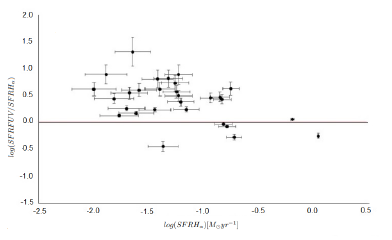
Fig. 3 Ratio of SFR(FUV)/SFR(H α ) vs. SFR(H α ). The solid line indicates when both values are the same. Most of the galaxies show a positive value for this ratio indicating that the SFR obtained from the UV continuum is larger than the SFR from H α with DIG.
The values of Table 3 show that the average star formation rates from Hα and FUV are very similar for the sample as a whole, as well as for the Sm galaxies, and there are only large differences for dS galaxies (a factor of 2.7). One explanation might be that the star formation event is older in the latter galaxies; therefore, all the massive stars which can ionize hydrogen have disappeared already, and the Hα flux is quite low. However, there are still a lot of less massive stars which can emit at FUV wavelengths, hence the large value of the SFR(FUV).
3.4.Bars and Star Formation Rates
It has been suggested that strong barred galaxies have larger SFRs (e.g. Sérsic & Pastoriza 1967; Ho et al. 1997; Tsai et al. 2013). However, other autors proposed that bars may decrease the SFR of a galaxy (e.g. Tubbs 1982; Kim et al. 2018). Kim et al. (2017), using a large sample of galaxies from SDSS, found out that barred galaxies have significantly lower star formation activity than their unbarred counterparts. Ryder & Dopita (1994) stated that the effect of the bar in the star formation rate is not important. Therefore, the problem is far from being settled yet.
We analized the effect of the existence of bars in the SFR of our sample. Barred galaxies represent 28% of the galaxies in our sample; therefore, the results are significant. Figure 4 shows the distribution of the SFR for barred and non-barred galaxies, with the average values presented in Table 3. Non-barred galaxies have larger SFR than barred ones from 𝐻 𝛼 values, while the SFR is similar when determined with FUV fluxes. However, the distributions are very different in both cases. Barred galaxies have a small range of SFR, with no large values (neither from Hα nor from FUV). The distribution of barred galaxies with FUV values is flat. From our sample it can be concluded that barred galaxies have a lower SFR than non-barred ones.
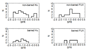
Fig.4. Star formation rate distribution for barred (bottom row) and non-barred galaxies (top row) in the sample. The left plots show the SFR determined with the Hα luminosity while the right plots show the distribution of the SFR determined with the FUV continuum. Non-barred galaxies have, on average, larger Star Formation Rates.
How can this influence the lower values of SFR for dS? Actually, the number of barred dS galaxies is small, only three out of 14; therefore, the results cannot be conclusive. However, there are no differences in SFR(Hα) while the differences increase for SFR(FUV). So, the small SFR for dS galaxies must be due to another reason.
3.5.Comparison with Previous Results
There are several studies of SFR involving late-type galaxies that use different diagnostic methods (e.g. Hunter & Elmegreen 2004; Hunter et al. 2010; Rosenberg et al. 2008; Lee et al. 2009; Buat et al. 2009; Boselli et al. 2015; Boselli et al. 2009; James et al. 2008; Almoznino & Brosch, 1996). In general, Sm galaxies have higher values than Im galaxies in all these investigations, with the values for the Im being closer to the SFR of our dS galaxies. On average, the SFR values reported for Sm galaxies are very similar to those we determined when extinction is considered. This is particularly important for the SFR(FUV), because the extinction is larger than in the optical range. This might be the main reason for the differences between our SFR(FUV) values and those reported by Lee et al. (2009) and Hunter & Elmegreen (2004), with the latter authors using the color excess and the extincion law of Cardelli et al. (1989) and the former ones using the Balmer decrement to determine the internal extinction. Therefore, our values are between two to five times larger than theirs.
Concerning the comparison between the SFR(Hα) and SFR(FUV), our results are similar to other investigations, the SFR(FUV) being higher than the SFR(Hα), except for the KISS sample by Rosenberg et al. (2008), where at least 8 out of 19 galaxies have lower SFR(FUV).
Eleven of the galaxies studied here have SFR values previously determined from
Hα emission (Hunter &
Elmegree, 2004; James et al.
2004; Lee et al. 2009; Van Zee, 2001), and four have previous FUV
emission determinations (Hunter & Elmegree,
2010; Lee et al. 2009). Six of
the values for SFR(Hα) are identical to our values, while another
five are similar when the uncertainties are considered. The most discordant
SFR(Hα) values are for UGC 9018, UGC 8385, DDO 18 and James et
al.’s value for UGC 11820. There are several reasons for such differences, among
others: the use of different distances or differences in the internal
extinction. For example, James et al.
(2004) adopted a constant value of 1.1 mag for the extinction of all
their galaxies, regardless of their morphological type or inclinations. This
value is higher than the extinction we reported in our § 3. Also, different
number of HII regions detected might change the value of the SFR, as in UGC
11820, where in a previous work up to 40 HII regions were considered, and a SFR
of
3.6.Star Formation Efficiency
Galaxies with distinct spiral arms, like Sc type, have larger SFR due to the fact
that they have a large amount of gas and a prominent density wave (Kennicutt, 1998). Late-type galaxies (Sm,
Im and dS) have, in general, smaller values of the SFR despite their large
amount of gas. However, when the SFR surface density is considered, galaxies
behave very differently. Hunter & Elmegreen
(2004), using a sample of Sm, Im and blue compact dwarf galaxies
(BCD), found out that the latter were the galaxies with the largest SFR surface
densities (see their Figure 5). A similar
result is found here, using the optical radius instead of the disk scale length
in V which, according to Hunter & Elmegreen
(2004), makes no difference for SFR surface densities lower than 0.05
Mʘ yr-1kpc-2. The SFR surface density for
dS galaxies is larger (with an average value of
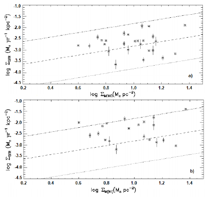
Fig.5. Correlation between the SFR surface density and the average surface densities of HI. The dashed lines correspond to constant global star formation efficiencies (1, 10, 100%) from Kennicutt (1998). The Sm and dS galaxies are shown with different symbols (stars and diamonds, respectively). The graph at the top shows the KS law when the star formation was determined from the Hα luminosity, while the one at the bottom shows the star formation determined with the FUV continuum.
In order to study this effect, the well-known Kennicutt-Schmidt law is applied to
our data and is presented in Figure 5 for
both Hα (top) and FUV (bottom). As no information is available on the
amount of molecular gas in these galaxies, the gas density was determined as
If the figure were divided into three different regions according to the efficiency, the number of Sm and dS galaxies would be very similar in all regions, but at intermediate/lower efficiency the Sm type would be slightly more numerous.
The larger amount of gas in Sm with a similar HI mass might indicate that they will form stars for a longer time than dS, or that they have started to form stars more recently than dS, but we do not have yet enough information to discriminate between these options.
4. Spatial Distribution of the Star Formation
The spatial distribution of the HII regions inside late-type galaxies was studied in previous investigations (e.g. Hodge 1969; Hunter & Gallagher 1986; Brosch et al. 1998; Sánchez & Alfaro 2008). Roye & Hunter (2000) concluded that, in irregular galaxies, the distribution of HII regions is mostly random, although the majority of the regions are concentrated in the central part of the galaxy. This is very similar to the previous results of Hodge (1969) and Brosch et al. (1998) who obtained a global asymmetry in the locations of the HII regions, with a concentration towards the center of the galaxies. On the contrary, Hunter (1982) found a random distribution of HII regions in late-type galaxies, with the exception of a few chains. Elmegreen & Elmegreen (1980) found that the largest HII regions in barred galaxies were located at the end of the bar. A study of the distribution of the HII regions within galaxies in our sample might help shed some light on the previous discussion. Moreover, the locations of the HII regions inside a galaxy might give information about possible previous interactions between galaxies.
In order to study if there is any particular distribution in the locations of the HII regions for the galaxies of our sample, we selected those galaxies with more than 10 HII regions (17 galaxies, 10 Sm and 7 dS) and inclinations lower than 70 to avoid problems of resolution and projection. From a quick inspection of the images (Hα shown in Figure 6 and broadband images not shown here) it can be concluded that only DDO 36, NGC 2552, UGC 6151 and UGC 6713 might have spiral arms, because the HII regions are strongly aligned along the structure of the galaxy. The regions inside UGC 6399 and UGC 891 are also aligned along the major axis, but as these galaxies have large inclinations, it might be just a projection effect. For the other 11 galaxies, the HII regions are randomly distributed.
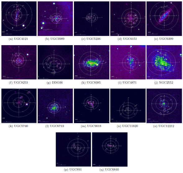
Fig. 6 Hα Images of those galaxies with a large number of HII regions. To study the spacial distribution of the HII regions we divided the galaxy into three concentric regions, which are marked with circles in the figures: inner, middle and outer regions, each representing 1/3 of the optical radius. The color figure can be viewed online.
4.1.Concentration Parameter
One parameter that can give us important information about the distribution of the star formation within galaxies is the concentration index (hereafter CI n ), which is defined as the ratio between the number of HII regions in the inner part and outer part of the galaxy (Roye & Hunter 2000). With this definition of the CI n , a value of 0 means that all HII regions are in the outer part of the galaxy, and the larger the CI n the more concentrated towards the center the regions are. In the determination of the CI n for the 17 galaxies selected before, we follow Roye & Hunter (2000); the values are listed in Column 2 of Table 4. All the galaxies have CI n s larger than 1, and four of them have CI n values larger than 10, indicating a large concentration of the regions towards the center. Only six of the galaxies have CI values smaller than 4, so their HII regions are located mostly outside the inner part. In general, it can be said that the galaxies in this subsample do not have their HII regions in their outskirts.
Tabla 4 Dsitribution of the star formation with radius
| CIn | CIf | Inner | Middle | Outer | ||||||||||
| Galaxy | n | %n | FHa10-14 [erg s-1 cm-2] | %F | n | %n | FHa10-14 [erg s-1 cm-2] | %F | n | %n | FHα10-14[erg s-1 cm-1] | %F | ||
| UGC4121 | 10.0 | 6.6 | 7 | 50.0 | 0.60 | 48.0 | 6 | 42.9 | 0.49 | 39.2 | 1 | 7.1 | 0.16 | 12.8 |
| UGC3989 | 2.0 | 3.8 | 3 | 18.8 | 0.37 | 31.1 | 6 | 37.5 | 0.42 | 35.3 | 7 | 43.7 | 0.40 | 33.6 |
| UGC5236 | 1.5 | 0.7 | 0 | 0.0 | 0.00 | 0.0 | 5 | 33.3 | 1.11 | 16.7 | 10 | 66.7 | 5.52 | 83.3 |
| UGC6151 | 7.2 | 1.7 | 4 | 28.6 | 0.34 | 28.0 | 7 | 50.0 | 0.59 | 48.9 | 3 | 21.4 | 0.28 | 23.1 |
| UGC6399 | 13.3 | 14.6 | 8 | 61.5 | 0.31 | 68.9 | 5 | 38.5 | 0.14 | 31.1 | 0 | 0.0 | 0.00 | 0.0 |
| UGC8253 | 3.0 | 2.9 | 4 | 28.6 | 0.41 | 26.1 | 5 | 35.7 | 0.55 | 35.0 | 5 | 35.7 | 0.61 | 38.9 |
| DDO36 | 4.0 | 3.0 | 0 | 0.0 | 0.00 | 0.0 | 11 | 42.3 | 1.05 | 47.9 | 15 | 57.7 | 1.14 | 52.1 |
| NGC2552 | 8.8 | 21.4 | 15 | 23.8 | 15.97 | 15.7 | 40 | 63.5 | 81.43 | 80.2 | 8 | 12.7 | 4.18 | 4.1 |
| UGC8385 | 5.1 | 9.0 | 8 | 47.1 | 5.25 | 62.9 | 5 | 29.4 | 1.53 | 18.3 | 4 | 23.5 | 1.57 | 18.8 |
| UGC4871 | 10.0 | 13.0 | 2 | 14.3 | 0.17 | 12.2 | 9 | 64.3 | 1.02 | 73.4 | 3 | 21.4 | 0.20 | 14.4 |
| UCG5740 | 9.0 | 7.7 | 8 | 61.5 | 1.72 | 42.5 | 3 | 23.1 | 1.63 | 40.2 | 2 | 15.4 | 0.70 | 17.3 |
| UCG6713 | 3.6 | 3.0 | 2 | 11.8 | 0.49 | 11.0 | 13 | 76.4 | 3.24 | 72.5 | 2 | 11.8 | 0.74 | 16.5 |
| UCG9018 | 8.8 | 19.2 | 7 | 43.8 | 3.24 | 56.6 | 7 | 43.8 | 2.06 | 36.1 | 2 | 12.5 | 0.42 | 7.3 |
| UCG11820 | 2.9 | 2.9 | 6 | 31.6 | 1.71 | 32.3 | 3 | 15.8 | 0.67 | 12.6 | 10 | 52.6 | 2.92 | 55.1 |
| UCG12212 | 3.0 | 4.5 | 6 | 28.6 | 8.47 | 41.9 | 9 | 42.8 | 7.21 | 35.6 | 6 | 28.6 | 4.55 | 22.5 |
| UGC891 | 17.3 | 25.2 | 7 | 43.8 | 3.58 | 43.3 | 9 | 56.2 | 4.69 | 56.7 | 0 | 0.0 | 0.00 | 0.0 |
| UCG6840 | 6.0 | 0.63 | 7 | 35.0 | 0.26 | 9.2 | 8 | 40.0 | 0.15 | 5.3 | 5 | 25.0 | 2.41 | 85.5 |
Galaxy name in Column 1. In Columns 2 and 3, the concentration rates are listed by number (CIn) and by flux (CIf ), respectively. Columns 4 and 5 list the number of HII regions and their percentages. Columns 6 and 7 contain the total Ha flux of these regions, and their percentage, within the innermost section of the galaxy. This section corresponds to a disk with a radius equal to one-third of R25. Columns 8 and 9 display the number of HII regions and their percentage. Columns 10 and 11 list the total Ha flux within the middle section of the galaxy and the corresponding percentage. This section corresponds to a ring with an outer radius equal to two-thirds to R25. Columns 12 and 13 show the number of HII regions and their percentage. Columns 14 and 15 list the total Ha flux within the outer section of the galaxy, and their percentage. This section corresponds to a torus with an outer radius equal to R25.
Another CI (hereafter, CI f ) can be defined using the flux of the HII regions (Fin/Fout) instead of the number of them. This is presented in Column 3 of Table 4. Again, large values of CI f indicate a large amount of flux towards the center, and small values indicate a large amount of flux from the outer regions. Eight of the galaxies have CI f smaller than 4; therefore their flux comes mostly from the outskirts. On the contrary, five galaxies have a strong luminosity from their center.
The most interesting result emerges when we compare both CIs. One might think that their values should be similar, e.g. if a galaxy has most of its HII regions in the inner part, then most of the flux of the galaxy (in Ha) should come from it as well. Thereupon, it could be said that the galaxy is “well balanced": there is more flux because there are more Hii regions. Such comparison can be done using Columns 2 and 3 of Table 4. Half of the sample has similar values of both concentration index. However, there are three galaxies (UGC 4121, UGC 6151, and UGC 6840) with much higher values of their CI n (a factor 1.5 or larger) than the CI f . Therefore these galaxies have a large number of regions inside their central region, but they are not very luminous. On the contrary, four of the galaxies in the sample (24 %) have a CI f much larger than the CI n , indicating that, despite being fewer in number, the regions in the center of the galaxy are brighter than those in the outskirts.
It can be concluded that the galaxies in this subsample have a larger number of HII regions in the inner half of the galaxy, and they are also more luminous than the regions in the outer half of the galaxy. However, this is intriguing because in a visual inspection of the galaxies (see Figure 6), the large number of the central HII regions and their dominance of the luminosity is not clear. Therefore, we divided the galaxy into three concentric regions: the inner region with a radius of 1/3 of the total optical radius, the middle region, a torus between 1/3 and 2/3 of the r25, and the outer region, from there up to the optical radius. They are marked with circles in Figure 6. The number of HII regions inside each of these regions, as well as their total flux, are listed in Table 4, Columns 4 to 15. There is no clear pattern, as can be seen in Figures 7 and 8, where the profiles of the number of HII regions (solid line) and the flux (dotted line), both normalized to the total number of regions (or flux) for each galaxy, are shown. The most peculiar profile might be the one of UGC 6840, with fewer regions in the inner annulus, dropping toward the middle section and increasing dramatically at the outer part of the galaxy. Moreover, this galaxy, along with UGC 3989, has the largest differences between the number and the flux distribution. Regarding the non barred galaxies, four out of 12 have the number and the flux of their HII regions concentrated in one of the annuli of the galaxy, while for other four the distribution is very uniform along the galactocentric distance. Four of the five barred galaxies have a large number of HII regions in the middle part of the galaxy. These results do not support the idea that bars inhibit the star formation in the central part (e.g. James & Percival, 2018; Tubbs 1982; Kim et al. 2018) because only DDO 36 has fewer regions inside its central annulus. It is interesting to note that all galaxies with a clear spiral structure have all -or almost all of their star formation regions concentrated in the middle and outer sectors of the galaxy, following the spiral arms. On the other hand, the regions of star formation in galaxies without, or with a not-so-well defined spiral structure, do not show any special distribution.
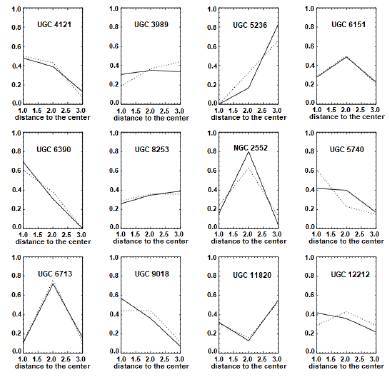
Fig. 7 Distribution of the number of HII regions (solid line) and their fluxes (dotted lines) along the distance to the center of the regions, for the non-barred galaxies. The y axis is the normalized number of HII regions (solid) or flux (dotted) of the galaxy and the x axis is the location of the galaxy in the any of the three regions we divided the galaxies into: inner, middle and outer part. Each galaxy has a different trend: some galaxies have more regions in the inner part, some others in the outer and some others in the middle. UGC 3989 has its star-forming regions quite homogeneously distributed along the radius, but the flux increases towards the edge. For most of the galaxies, the number of regions and the associated fluxes mimic each other.
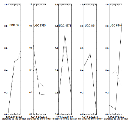
Fig. 8 Distribution of number of H II regions (solid line) and their fluxes (dotted line) along the radius for barred galaxies. Only two of them have most of their regions and flux in the middle part of the galaxy, where the bar is expected to end, and to have an important influence on the star formation. Axis as in Figure 7. From left to right the galaxies are: DDO 36, UGC 8385, UGC 4871, UGC 891 and UGC 6840.
From these figures and the values in Table 4 it can be concluded that the HII regions of the galaxies in our sample show a variety of distributions, more similar to a random behavior than to a clear pattern, as observed in spiral galaxies.
4.2.Asymmetry of the HII Region Distribution
In a recent study of the dwarf, interacting spiral galaxy IC 1727, it was found that the largest and brightest of its HII regions are facing the companion galaxy, NGC 672 (Ramirez-Ballinas & Hidalgo-Gámez 2014). We aim to check if the HII regions are located in a particular zone in the galaxy, because such an accumulation of the star formation in one particular direction might indicate an interaction. There are two possible approaches: the asymmetry index AI, (Roye & Hunter, 2000), or a simpler one: to just check if there is any preferred locus of star formation inside each galaxy, dividing these into the four orientations, as was done for IC 1727. We will first consider the latter approach. To proceed, the 17 galaxies studied in the previous subsection were divided into four directions: NE, NW, SE and SW (North is up and East to the left). The values of the number of HII regions and the fluxes for each quadrant are listed in Table 5. Half of the galaxies in the sample have a quadrant (or two) with a meaningful increase in the number of HII regions (larger than 35%). This might indicate a previous interaction. Moreover, two of them, both barred galaxies, have the majority of regions in opposite quadrants, while another four galaxies have them in adjacent quadrants. A likely explanation might be that star formation is due to gas coming out along the bar, as seen in other galaxies (Sérsic & Pastoriza 1967; Ho et al. 1997).
Tabla 5 Distribution of the star formation in orientation
| Ne | NW | SE | SW | AInAIf | ||||||||||||
| Galaxy | n | %n | FHa10-14 [erg s-1 cm-2] | %F | n | %n | FHa10-14 [erg s-1 cm-2] | %F | n | %n | FHa10-14 [erg s-1 cm-2] | %F | n | %n | FHa10-14 [erg s-1 cm-2] | %F |
| UGC4121 | 3 | 21.4 | 0.26 | 21.8 | 5 | 35.8 | 0.46 | 38.7 | 3 | 21.4 | 0.27 | 22.7 | 3 | 21.4 | 0.20 | 16.8 0.75 0.65 |
| UGC3989 | 4 | 25.0 | 0.22 | 18.6 | 4 | 25.0 | 0.37 | 31.4 | 4 | 25.0 | 0.37 | 31.4 | 4 | 25.0 | 0.22 | 18.6 1.00 0.75 |
| UGC5236 | 1 | 6.7 | 0.24 | 3.6 | 6 | 40.0 | 2.65 | 40.0 | 2 | 13.3 | 2.80 | 42.2 | 6 | 40.0 | 0.94 | 14.2 0.50 0.85 |
| UGC6151 | 2 | 14.3 | 0.16 | 13.5 | 2 | 14.3 | 0.18 | 15.0 | 5 | 35.7 | 0.45 | 37.4 | 5 | 35.7 | 0.41 | 34.1 0.56 0.56 |
| UGC6399 | 2 | 15.3 | 0.12 | 26.0 | 5 | 38.5 | 0.17 | 37.0 | 6 | 46.2 | 0.17 | 37.0 | 0 | 0.0 | 0.00 | 0.0 0.86 0.84 |
| UGC8253 | 5 | 35.7 | 0.53 | 34.0 | 2 | 14.3 | 0.18 | 11.5 | 4 | 28.6 | 0.49 | 31.4 | 3 | 21.4 | 0.36 | 23.1 0.75 0.65 |
| DDO36 | 7 | 26.9 | 0.44 | 20.1 | 2 | 7.7 | 0.34 | 15.5 | 9 | 34.6 | 0.46 | 21.0 | 8 | 30.8 | 0.95 | 43.4 1.00 0.90 |
| NGC2552 | 12 | 19.0 | 22.40 | 22.2 | 11 | 17.5 | 16.46 | 16.4 | 17 | 27.0 | 31.15 | 31.0 | 23 | 36.5 | 30.58 | 30.4 0.98 0.98 |
| UGC8385 | 3 | 17.6 | 0.76 | 9.1 | 5 | 29.5 | 1.89 | 22.6 | 4 | 23.5 | 1.18 | 14.1 | 5 | 29.4 | 4.52 | 54.2 0.89 0.46 |
| UCG4871 | 4 | 28.6 | 0.26 | 18.7 | 5 | 35.7 | 0.62 | 44.6 | 2 | 14.3 | 0.17 | 12.2 | 3 | 21.4 | 0.34 | 24.5 0.56 0.57 |
| UCG5740 | 1 | 7.7 | 0.23 | 5.7 | 7 | 53.8 | 2.75 | 67.9 | 3 | 23.1 | 0.53 | 13.1 | 2 | 15.4 | 0.54 | 13.3 0.86 0.87 |
| UGC 6713 | 4 | 23.6 | 0.41 | 9.2 | 7 | 41.2 | 2.59 | 57.9 | 3 | 17.6 | 0.41 | 9.2 | 3 | 17.6 | 1.6 | 23.7 0.70 0.55 |
| UCG9018 | 5 | 31.3 | 1.20 | 20.9 | 2 | 12.4 | 0.45 | 7.9 | 4 | 25.0 | 1.73 | 30.2 | 5 | 31.3 | 2.35 | 41.0 0.78 0.57 |
| UCG11820 | 5 | 26.3 | 1.58 | 30.2 | 10 | 52.6 | 2.72 | 52.0 | 1 | 5.3 | 0.21 | 4.0 | 3 | 15.8 | 0.72 | 13.8 0.90 0.73 |
| UCG12212 | 5 | 23.8 | 4.56 | 22.3 | 2 | 9.5 | 3.36 | 16.5 | 6 | 28.6 | 6.01 | 29.5 | 8 | 38.1 | 6.46 | 31.7 0.91 0.88 |
| UCG891 | 9 | 56.2 | 5.14 | 62.1 | 1 | 6.3 | 0.00 | 0.0 | 1 | 6.3 | 1.22 | 14.8 | 5 | 31.2 | 1.91 | 23.1 0.78 0.52 |
| UCG6840 | 7 | 35.0 | 0.24 | 8.6 | 3 | 15.0 | 0.02 | 0.7 | 3 | 15.0 | 0.07 | 2.5 | 7 | 35.0 | 2.49 | 88.2 1.00 0.12 |
Galaxy name in Column 1. Columns 2 and 3 list the number of HII regions within the northeastern quadrant (NE) and their percentage. Column 4 shows the total H a flux of these regions, its percentage is listed in Column 5. In the same way, the number of HII regions (n), the corresponding percentage (%n), the total Ha flux of these regions and its percentage (%F), are presented for the quadrants northwest (NW), southeast (SE) and southwest (SW). The asymmetry indices by number (AIn) and by ux (AIf ) are shown in Columns 18 and 19.
The asymmetry index, based on the number of HII regions (AIn), is
defined as the ratio between the number of regions in the poorest side and the
richest side. An AI by number (or by flux, see below) equal to one means that
the galaxy is perfectly symmetric along that axis (major or minor axis), that
is, we have the same number of HII regions on both sides. On the contrary, an AI
of 0 means that all HII regions are concentrated on only one side of the galaxy.
We used our images in V and R to determine the major and minor axes and counted
the number of HII regions on each side of the axes. We decided to proceed as in
Roye & Hunter (2000), where they
a posteriori chose the axis (major or minor) with the largest symmetry. The
AIn values are shown in Column 18 of Table 5. We found that 80% of the galaxies in the sample
have an
As previously done with CI, an asymmetry index based on the flux can be determined as the ratio between the flux of all the regions on one side and the flux on the other side (AI f ) (AI f ). This index is shown in Column 19 of Table 5. Again, our galaxies appear to be very symmetric: only two of them have . According to the AI, most of the galaxies in our sample are predominantly symmetric in both the distribution of the HII regions, and their luminosity.
5. Is a Starburst Always a Starburst?
Several authors (e.g. Kennicutt 1998; Lee et al. 2009; Gilbank et al. 2010) claimed that the Ha photons from outside the HII regions, the so-called diffuse ionized gas (hereafter DIG), can also be used in the SFR determination because this gas is ionized by photons created by OB stars and they are emerging from the HII regions, since the nebulae are density bounded instead of radiation bounded. However, this is not always the case. There are many other processes which can ionize this gas, which are not related to young stellar population, such as shock waves (Rand 1998), turbulent mixing layers (Slavin et al. 1993), hot low-mass evolved stars (Flores-Fajardo et al. 2011), and radiation from WR stars (Hidalgo-Gámez 2005).
It is not easy to know which is the most important ionizing source for a particular galaxy and how much of the Hα luminosity comes from each of the sources using only Hα images. If other processes are at work for the ionization of the DIG, the SFR might be overestimated for those galaxies with a large amount of DIG. One example might be the irregular dwarf galaxy IC 10, which is considered to be a starburst galaxy based on its color (Richer et al. 2001), the high content of WR stars (Massey & Holmes 2002) and the large number of HII regions (Hodge & Lee 1990), with a SFR of about 1Mʘyr-1 (Zucker 2005). However, there is a strong emission from the DIG inside this galaxy, and up to 50% of this DIG is ionized by sources other than leaked photons (Hidalgo-Gámez 2005). Therefore, IC 10 might not be considered as a starburst galaxy (Hidalgo-Gámez & Magaña-Serrano 2017). The inclusion of the DIG within the Hα luminosity used in the SFR should overestimate the values and it can be risky, unless it is well known that leaked photons are the only source responsible for the ionization of this gas.
Unfortunately, the amount of DIG cannot be known in advance for a particular galaxy. Then, we decided to use previous studies on the DIG in late-type galaxies (e.g. Hidalgo-Gámez 2006; Hidalgo-Gámez, 2007; Hidalgo-Gámez 2005; Hidalgo-Gámez & Peimbert 2007) to determine the boundary flux between an HII region and the DIG. We estimate this flux to be of the order of 10-17erg cm-2 s-1. Then, we extracted the part of the Ha emission with fluxes larger than this value and a new SFR was determined from the new luminosities. The results are listed in Column 10 of Table 3. A quick comparison can be done between Columns 6 and 10 and it is shown in Figure 9. The number of galaxies with differences in the SFR when DIG is not included is quite large. For a total of 21 out of 36 galaxies in the sample, the SFR without the DIG is 50% lower than with it. There is no real differences between Sm (64%) and dS (53%). For seven of these galaxies the differences in the SFR with and without DIG amount to 90%. Probably, as these are late-type galaxies with a large amount of gas, the contribution of the gas between the Hii regions to the star formation rate is larger and, before including it in the calculation, a careful study on the ionization source of such gas should be done.

6. Conclusions
In this work, the star formation rates for a sample of late-type galaxies, Sm and dwarf spirals, have been determined. It is the first estimation of the star formation rate for more than half of the sample considered here. The SFR were determined using the Hα flux for 36 galaxies and the FUV flux only for 30 of them. The fluxes used, both Hα and FUV, were corrected for internal and external extinctions.
The bulk of the galaxies in our sample have SFRs lower than 0.1 Mʘ yr-1 for both diagnostic methods. These values are common for late-type galaxies. It is interesting to notice that SFR(FUV) is normally larger than the SFR determined with Hα. However, the largest SFRs were obtained from the Hα luminosities.
We also noticed a difference in the SFR between Sm and dS galaxies in the sense that the former had higher SFR values than dS with both methods.
If dS galaxies are not only smaller than Sm but a later type of galaxy intermediate between Sm and Irr galaxies, their lower SFR could be explained by an older star formation event for the dS galaxies. However, when the density of SFR (SFR/kpc2) is considered, both types of galaxies have similar values. These are values similar to those found before (e.g. Hunter & Elmergreen 2004), although the dispersion in our sample is larger.
We studied the role played by the bars as drivers of star formation in late-type galaxies and noticed that non-barred galaxies always have larger SFR than barred ones. Also, we studied the influence of the spiral arms in the SFR and found that, for late-type galaxies, the spiral wave might be not that important, and that other mechanisms might trigger star formation, as in irregular galaxies.
Considering the star formation efficiency, both types of galaxies have a similar efficiency of star formation, despite the greater amount of gas in the Sm and the differences in their gas mass densities.
We also studied the distribution of the HII regions for those galaxies in our sample with the largest number of regions. We used two approaches: the concentration and asymmetry indexes as in Roye & Hunter (2000) and a more detailed distribution with smaller divisions. We concluded that late-type galaxies are very symmetric and have their regions quite concentrated. Moreover, although there is a gradient in the number and the fluxes of HII regions for more than half of the galaxies studied, such gradient is not unique, being positive or negative for some galaxies and even with two slopes in others.
Finally, we noticed that the inclusion of the DIG within the estimation of the Hα luminosity might increase the SFR values more than previously thought. Therefore, the Hα luminosity should not be included unless it is well known that leaking photons from the Hii regions are the only source of the ionization.

