


 nova página do texto(beta)
 Inglês (pdf)
 Artigo em XML
 Referências do artigo
 Enviar este artigo por email
 Citado por SciELO
  Similares em
SciELO
Similares em
SciELO 
 Permalink
1. INTRODUCTION
The internet revolution has changed in a powerful and effective way how research is conducted today. Far away are the days when a researcher had to spend an incalculable amount of time in libraries searching and deciphering an ever growing and complex scientific literature. In this day and age, researchers’ primary reflex is to use the internet to search for and gather essential information to the advancement of their research. Astrophysics has been particularly at the forefront in adopting this technology and applying it to very diverse goals.
Services such as the ADS1 [SAO/NASA Astrophysics Data System Abstract Service (McKiernan 2001)] now play an indispensable role in providing easy access to millions of abstracts and to the associated papers.
Other web services have been created to facilitate the search of astrophysical data. A prominent example is the conglomerate of CDS2 (Strasbourg Astronomical Data Center) services like VizieR3, which became available in 1996 and was later described in Ochsenbein et al. (2000). It provides access to the most complete online library of published astronomical catalogues and data tables organized in a selfdocumented database system.
Another service from the CDS is the ALADIN4interactive sky atlas (Bonnarel et al. 2000; Boch & Fernique 2014), which allows simultaneous access to digitized images of the sky, astronomical catalogs, and databases. It is mainly used to facilitate direct comparison of observational data at any wavelength with existing reference catalogs of astronomical objects.
While such services have proven to be valuable, other areas of astrophysics can also benefit from those innovations. This is particularly the case of computational models such as photoionization and shock models computed using various spectral synthesis codes. Most of those models available in the ‘market’ can be found in the form of tables that are scattered around in the published literature. The most recent model grids are available as compressed files in multiple websites that use quite different data-formats. A centralized database, readily accessible and user friendly, would no doubt be beneficial to the community. To this end the Mexican Million Models database (3MdB5) was created (Morisset et al. 2015). It is designed to store and distribute photoionization models computed with the code cloudy (Ferland et al. 2017) using the MySQL database management system. This service offers to the community an easy access to millions of online models by means of the SQL language.
This paper deals with the addition of shock models calculated with the code mappings (Sutherland & Dopita 2017). This new database which includes shock models is called “3MdBs” (i.e., 3MdB-shocks). The structure of the 3MdBs database differs from the original 3MdB (photoionization models), but the logic behind its usage has remained the same. Both databases are available at the same address and both can be used simultaneously with the appropriate SQL queries. 3MdBs includes a website6 that allows one to explore the grid available in the database interactively, using a simple web browser. The website also contains tutorials allowing potential users to obtain the necessary information required to interact with it.
This paper is structured as follows. In § 2 we briefly introduce the modeling code mappings. § 3 explains the database structure. The grids of models available at the time of publication are presented in § 4 followed by a discussion about specials grids in § 4.4.
2. THE MODELING CODE
All the models referred to in this paper have been calculated using the shock and photoionization code mappingsv7, version 5.1.13 (Sutherland & Dopita 2017; Sutherland et al. 2018). The latest improvements made in mappingsv are detailed in Sutherland & Dopita (2017).
2.1. Preionization
Preionization conditions of the gas entering the shock front are an essential parameter of the shock calculations since they greatly influence the ionization structure of the shocked gas downstream and therefore all the line emissivities and their spatially integrated intensities (Dopita & Sutherland 1995; Allen et al. 2008). Manually setting preionization would be arbitrary and far from optimal, in particular in models related to specific astrophysical situations.
Allen et al. (2008), for instance, used an iterative process to determine preionization by first integrating the upstream propagating UV radiation, which is produced by the shocked gas UV emission downstream, and second, by using the resulting UV energy distribution to calculate a photoionization model for the preshock gas as it travels towards the shock front. In the case of high velocity shocks, it is a reasonable to assume that the precursor is photoionised and in near-equilibrium conditions, as determined from the ionizing radiation field generated by the shocked gas downstream.
Since there is a strong feedback between preionization conditions and the ionization of the shocked gas downstream and its UV emission, the adopted methodology consisted in repeating the shock calculations using the preionization conditions inferred from the previous shock iteration. By repeating this iterative procedure up to at least four times, one finds that both the temperature and ionization state of the precursor converge towards a stable value; hence, so will the line emission intensities of the cooling shock.
While this method is valid for shock velocities V s in excess of ≈ 200 km s−1, it fails for slower velocities since there is insufficient time for the preshock gas to achieve equilibrium before it is shocked. In such cases, it is essential to take into consideration the time dependent aspects of the problem. mappingsv now addresses the preionization problem in a fully consistent manner. For the first time, the new code treats the preshock ionization and thermal structure iteratively by solving, in a fully time-dependent manner, the photoionization of the preshock gas, its recombination, photoelectric heating and line cooling as it approaches the shock front. A detailed study of preionization in radiative shocks was presented in Sutherland & Dopita (2017). Therefore, the models in the database make use of this new treatment, in which the preshock temperature and ionization state of the gas are iteratively calculated after each shock calculation.
2.2. Precursor Gas
For shocks with a velocity of less than 100 km s−1, we did not compute the emission of the precursor since shocks below this velocity are unable to produce any appreciable ionizing emission. For shocks with velocity greater than 100 km s−1, the photoionized precursors were computed separately. These were evaluated after the ionizing radiation field generated by the shock had been computed. All precursors were calculated subsequently to each iteration using the option ‘P6’ in mappingsv (photoionization model), the ionizing radiation emanating from the shock being the only source of ionization in the current grid. We essentially used the exact same method employed by Allen et al. (2008) to compute the precursor emission spectrum.
3. THE NEW DATABASE
All models presented in this paper are stored into an SQL8 database freely available online. This method of distribution has three main advantages. First, it allows anyone to have access instantaneously to thousands of models without the hassle of installing and managing the database on one’s own workstation. Second, any new database updates or additions become instantly available to the community, a feature which can be very useful when it involves a worldwide collaboration (which is not available when using the VizieR database system). Third, the database can be accessed and handled using anyone’s preferred programming language as long as it includes a SQL client library.
In order to make use of this database and fully exploit its capabilities, the user needs to be familiar with the SQL database language, a domain-specific language designed for managing data stored in a relational database management system. This work makes use of MariaDB®, a fast, scalable and robust open source database server. In the following section, we shall explain the database structure and the variables it manages. This will be followed by a book case example of how the database is best used.
3.1. Database Structure
As in any database design, the data in distributed across several tables with a multicolumn setup. The whole database consists of 12 tables, each having a specific purpose, which we shall discuss in details below. An overall view of the database’s structure is displayed in Figure 1, which illustrates the different relations between the tables. The architecture adopts a modular design in the form of multiple tables, all with the aim of satisfying three criteria: efficiency, simplicity and expandability. By design, an SQL database can only contain a given number of name columns, depending of its configuration. Too many columns in a table can greatly degrade its performance, and even make it unstable. It is also very rare that one needs the information contained in all tables through a single database request. Most of the time, only a fraction of the table columns are needed at a given time. For this reason, the data are scattered into different tables, each having a specific purpose, while limiting data duplication and thus optimizing the database size.
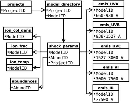
All the shock parameters are found in the table named shockparams (Table 4). This table includes various columns associated with the shock parameters described in § 4.1, mainly the shock velocity (shc-kvel), the preshock density (preshck_dens) and the transverse magnetic field (magfld). The abundance sets used for a specific model are referenced using an abundance identification code (AbundID), which is linked to the table abundances that contains a list of all abundance sets available in the database at the time it is consulted.
A total of 4132 emission lines from ultraviolet to infrared can be extracted from the database. They are distributed among 5 tables, each covering specific wavelength intervals : 660-938 Å (emisUVA), 939-1527 Å (emisUVB), 1528-2999 Å (emisUVC), 30007499 Å (emis_VI) and 7500Å-609µm (emis_IR). The complete emission lines list can be consulted via the web interface.
For each emission line of every model, the line intensities corresponding to the three different region types (namely shock, precursor and shock+precursor) are available, using the filter WHERE emisVI.modeltype="shock" or "precursor" or "shockplusprecursor" respectively.
The mean temperatures, weighted by the ionic fraction of the specie involved, are given for each model in the table tempfrac, with the average ionic fraction listed in the column labelled ionfrac and the ionic column densities in the column ioncolumnfrac.
There are two more tables in the database that are usually not expected to be required. Their names are projects and models_directory. They ought to be used only when one needs to reevaluate a model, or when the latter contains information required by the web-interface.
3.2. Website and User Credentials
In § 4, we describe the models grids available at the time of publication. With time, other grids will be calculated and added in the database. In order to publicize these grids to the community, we created a website allowing to visualized the different grids available at the time of consultation. The website can be reached via http://3mdb.astro.unam.mx/.
The user credentials can be obtained via the website along with the IP adress and port needed to connect to the database.
The website is connected directly to the MariaDB9 database. This means that it is adaptive, and any changes made to the database will automatically appears in the different sections. New grids of models can be added to the database, which then become automatically visible and accessible to the general public. Since each grid is built using a distinct range of shock parameters, and the spacing between successive values is at times non-uniform from grid to grid, the website provides a parameter explorer that allows any user to explore the database and, in an intuitive manner, to compose relatively complex SQL queries, such as the one given as example in Table 1. The website also includes interactive tutorials that aim at teaching any user how to connect and interact with the database using the Python programming language.
4. THE MODEL GRIDS IN THE DATABASE
At the time of publication, 3 main grids are available in the database :
An exact replica of the Allen et al. (2008) grids (§ 4.1).
An extension of the Allen et al. (2008) gridscomputed for low metallicities using the abundances of Gutkin et al. (2016) (§ 4.3)
An extension of the Allen et al. (2008) gridscomputed for different shock ages (§ 4.4).
Not all the parameter grids presented in this paper are equally set in the shock parameter space (i.e., the size of the intervals and the range they cover may depend differently on the assumed abundances). The next section will describe the grids of models currently available in our database. For all models of the grid, we provide information about each of the three regions: shock, precursor and shock+precursor. The effect of dust has not been considered in the models.
4.1. The Allen et al. (2008) Grid
As in Allen et al. (2008), each shock model from the grid is uniquely defined through five different input parameters: the shock velocity V s , the preshock transverse magnetic field B 0, the preshock density n 0 and one of the five abundance sets listed in Table2. The temperatures of the ions and electrons have been set to be equal right from the shock front. The ionization state of the precursor (the gas entering the shock front) is calculated with mappingsvusing the method described in § 2.1.
The grid is divided into two sub-grids. Both of which are an exact replica of those presented by Allen et al. (2008), as they use the same shock parameters. The only exception is the use of mappingsv instead of mappingsiii during model evaluations. Below is a summary of each sub-grid.
The first sub-grid contains 1440 models that were calculated using one of the following five abundance sets: a depleted solar set and a twice-solar set, which were both used by Dopita & Sutherland (1996), a solar abundance set labelled ‘dopita2005’ from Asplund et al. (2005)), which was used in Dopita et al. (2005), and finally, an SMC and an LMC abundance set published by Russell & Dopita (1992). The respective abundances for each atomic element with respect to hydrogen are given in Table2. Each model in this sub-grid was calculated using a fixed preshock density of n 0 = 1 cm−3 consisting of 36 individual shock velocities (from 100 up to 1000 km s−1 in steps of 25 km s−1) and one of the following 8 transverse magnetic field values: B = 10−4, 0.5, 1.0, 2.0, 3.23, 4.0, 5.0 and 10 µG.
TABLE 1 EXAMPLE OF SQL COMMAND LINES USED TO GENERATE FIGURE 2
|
TABLE 2 ABUNDANCES USED IN ALLEN ET AL. 2008
| Elem | Solar | 2×Solar | Dopita2005 | LMC | SMC |
|---|---|---|---|---|---|
| H | 0.00 | 0.00 | 0.00 | 0.00 | 0.00 |
| He | -1.01 | -1.01 | -1.01 | -1.05 | -1.09 |
| C | -3.44 | -3.14 | -4.11 | -3.96 | -4.24 |
| N | -3.95 | -3.65 | -4.42 | -4.86 | -5.37 |
| O | -3.07 | -2.77 | -3.56 | -3.65 | -3.97 |
| Ne | -3.91 | -3.61 | -3.91 | -4.39 | -4.73 |
| Na | -6.35 | -4.85 | -5.92 | ||
| Mg | -4.42 | -4.12 | -5.12 | -4.53 | -5.01 |
| Al | -5.43 | -5.23 | -7.31 | -4.28 | -5.60 |
| Si | -4.45 | -4.15 | -5.49 | -5.29 | -4.69 |
| S | -4.79 | -4.49 | -5.01 | -5.23* | -5.41 |
| Cl | -6.70 | -7.30 | |||
| Ar | -5.44 | -5.14 | -5.44 | -5.71 | -6.29 |
| Ca | -5.88 | -5.58 | -8.16 | -6.03 | -6.16 |
| Fe | -4.63 | -4.33 | -6.55 | -4.77 | -5.11 |
| Ni | -7.08 | -6.04 | -6.14 | ||
| X | 0.7073 | 0.6946 | 0.7158 | 0.7334 | 0.7535 |
| Y | 0.2745 | 0.2696 | 0.2778 | 0.2596 | 0.2432 |
| Z | 0.0183 | 0.0358 | 0.0065 | 0.0070 | 0.0033 |
*A typo error shows -7.23 in the Allen et al. (2008) paper although their model was obtained with the correct value of -5.23, as the one present in the grid.
The second sub-grid of models was calculated using only the solar abundance set of Dopita & Sutherland (1996) with 6 preshock densities (0.01, 0.1, 1.0, 10, 100 and 1000 cm−3), at 36 shock velocities (100 up to 1000 km s−1 in steps of 25 km s−1) and for 8 transverse magnetic field values (B = 10−4, 0.5, 1.0, 2.0, 3.23, 4.0, 5.0 and 10 µG). As in the Allen et al. (2008) paper, further models were computed using additional values of B in order to cover all the magnetic parameter values B/n 1/2 from the first subgrid. This facilitates comparison of models that differ by their preshock density. We recall that models with the same ratio B/n 1/2 result in the same magnetic to gas pressure ratio. These additional values (transverse magnetic field) are B ≈ 10−3, ≈ 10−2, ≈ 10−1, 1.0, 10 and 100 µG, and were calculated for each selected preshock density.
4.2. Comparison Between the Allen 2008 Models and Our Calculations
The first application of the new model grid was to compare it with the previous grid from Allen et al. (2008). Figure 2 shows a classical plot of [O III]/Hβ versus [N II]/Hα, commonly known as a BPT diagnostic diagram (Baldwin et al. 1981). Except for the fact that our grid was computed using the code mappingsv, it is otherwise equivalent to the one presented by Allen et al. (2008). We assumed the same shock parameters: a solar abundance set with shock velocities varying from 200 to 1,000 km s−1. The transverse magnetic field covers the range 0.0001 to 2 µG and the preshock density is always 1 cm−3. The left panel displays the line ratios from the shocked gas only, while the right panel displays the same ratios after summing up both shock and precursor line intensities. Our figure can be directly compared to Figure 20 of Allen et al. (2008).
Figure 3 shows a direct comparison between our grid (blue lines) and the Allen et al. (2008) version using MAPPINGS III(gray lines). Although similarities do appear between the different line ratio curves, higher value by up to ≈ 0.3 dex of our [O III]/ Hβ ratio shows up in some parts of the diagram.
Figure 4 displays the behavior as a function of shock velocity Vs of 16 different emission lines. These further illustrate the similarities and differences between both grids of models. All lines are normalized to the Hβ intensity. Colors represent whether the emission comes from the shocked gas only (red), from the preshock gas (green) or from the sum of both (blue). The models using are shown using dotted lines while the continuous lines represent the Allen et al. (2008) models. For both grids, a preshock density of 1cm−3 and a magnetic field of 3.23 µG were assumed. The color shaded bands represent the range in flux variations within the mappingsv grid when the magnetic field is varied between 10−4 and 10µG.
We note from Figure 4 that the behavior of the emission line intensities is quite similar in the mappingsv and mappingsiii grids, although significant differences appear for the lines [C IV] 1550Å, C III] 1909Å, [O III] 4363Å, [O III] 5007Å, and [Ne V] 14.3µm, which are predicted stronger in our new grid, while the lines [C II] 2327Å and [Ne III] 15.5µm are predicted weaker. Other lines appear stronger or weaker depending on the shock velocity considered.

Fig. 2 The BPT [O III] λ5007/Hβ versus [N II] λ6583/ Hα diagnostic diagram (Baldwin et al. 1981) displaying shock models that use the same abundance sets as Allen et al. (2008) and which cover shock velocities ranging from 200 to 1000 km s−1, all with the same preshock density of n0 = 1 cm−3. The left panel displays the line ratios from the shocked gas only while the right panel shows the same ratios after summing up shock and precursor line intensities. This figure is identical to Figure 20 shown in Allen et al. (2008), except that the models shown here were calculated with instead of MAPPINGS III. The color figure can be viewed online.
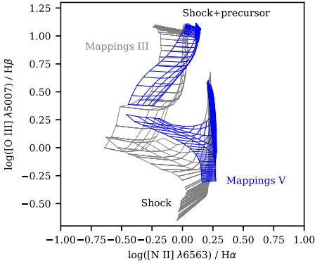
Fig. 3 Comparison of mappingsiii and mappingsv in the BPT diagram of [O III] λ5007/Hβ vs. [N II] λ6583/Hα when using the same model parameters as Allen et al. (2008): a solar abundance set, a preshock density of n 0 = 1 cm−3, shock velocities ranging from 200 to 1000 km s−1 with an interval of 25 km s−1, and a transverse magnetic field of 10−4, 1, 2 and 4 µG cm 3/2 . The models calculated by Allen et al. (2008) are shown in gray and our models using mappingsv are shown in blue. This figure is similar to Figure 21 of Allen et al. (2008), which was used by the authors to compare their mappingsiii grid to an earlier grid from Dopita & Sutherland (1996). The color figure can be viewed online.

Fig. 4 Line fluxes as a function of shock velocity for 16 emission lines, normalized to Hβ. Colors represent whether the emission is from the shocked gas only (red), or from the preshock gas (green) or from the sum of both (blue). The models using mappingsv are shown using dotted lines while the continuous lines represent the Allen et al. (2008) models. The color-shaded bands represent the domain of line intensity variations of the mappingsv grid when gradually varying the magnetic field from 10−4 to 10µG (with the same color coding as for the dotted lines). The color figure can be viewed online.
Figure 5 is another illustration of the differences between the Allen et al. (2008) models and the current grid. The six panel pairs represent useful line ratio diagnostics when studying LINERs. All the sequences shown are from our grid only and they all have the same transversal magnetic field of 1µG. The emission lines in the left panels represent shocked gas only, while those in the right panel represent the sum of shock with precursor emission lines. The model sequences shown correspond to sequences in which either the precursor density (red lines) or the shock velocity (blue lines) were varied. The line thickness (of the red and blue lines) increases as the iso-parameter takes on larger values. These models are equivalent to those presented by Molina et al. (2018) in their Figures 24 to 29. The main difference found in our grid is the [O III] 5007Å line, which can be up to 0.3dex stronger than in Molina et al. (2018).
The line ratio differences discussed above between code versions arise either from changes implemented in the newer mappings code or from the use of a more recent atomic database. It is beyond the scope of this paper (and of the authors’ expertise) to determine which of these is at play in any specific line intensity difference.
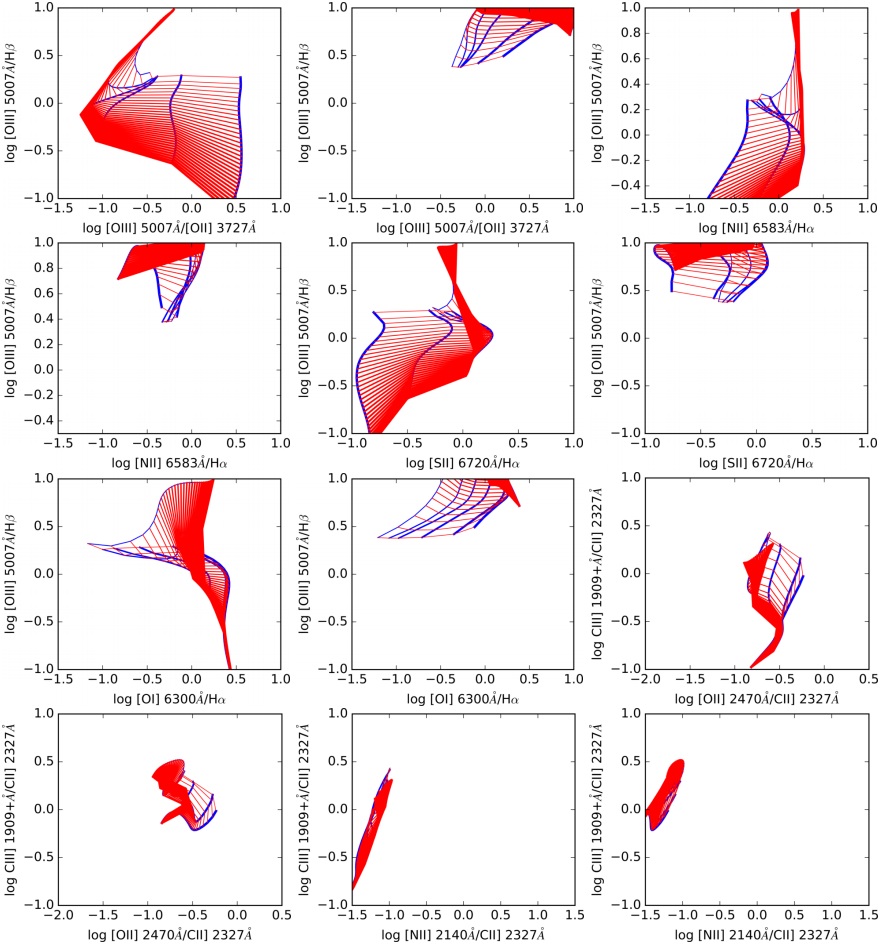
Fig. 5 Diagnostic diagrams to be compared to Molina et al. (2018), who used the Allen et al. (2008) models. All models shown have the same transverse magnetic field of 1µG. Red lines represent shock model sequences of different n 0 values but of equal velocity, while blue lines represent shock model sequences of different V s but of equal precursor density. The line thickness (of the red and blue lines) increases from one sequence to the next: the blue lines become thicker as the density increases and the red lines become thicker as the velocity increases. The color figure can be viewed online.
4.3. The Low Metallicity Grid
We have extended the grid of Allen et al. (2008) to include low metallicity abundances in order to study shocks in galaxies at different cosmic epochs. The abundance sets chosen for this grid in particular are the same as the ones derived in Gutkin et al. (2016), which were evaluated for different mass fraction of Z. We follow the same methodology as these authors, in order to retrieve the abundance of each individual element, from hydrogen to zinc.
Our database currently contains models calculated using the parameters given in Table 3. Figure 6 allows us to visualize the effect on the BPT diagram [O III]/Hβ vs. [N II]/Hα of adopting lower values of Z, starting with a value of (C/O)/(C/O)⊙ = 1 and successively going down to 10−4 (shifting from left to right in the figure). Interestingly, when the metallicity decreases, the horizontal spread of [N II]/Hα in each sequence tends to become narrower. Both changes of the shock velocity (from 100 to 1000km/s) and the magnetic field (from 10−4) to 10 µG) lead to an increase in [O III] 5007Å/Hβ, while [N II] 6583Å/Hα remains essentially constant. It is also apparent from these figures that very low metallicity shocks lead to very low values of any collisionally excited line when normalized with respect to a recombination line of H. It is important to keep in mind that at the very low metallicity end, the lines from metals become negligible, but the hydrogen and helium recombination or collisionally excited lines are still emitted. If such shocked gas emission were superposed on the observation of a photoionized region, it might lead to an underestimation of metallic abundances, which would unavoidably result from simply assuming classical methods to determine e.g. O/H.
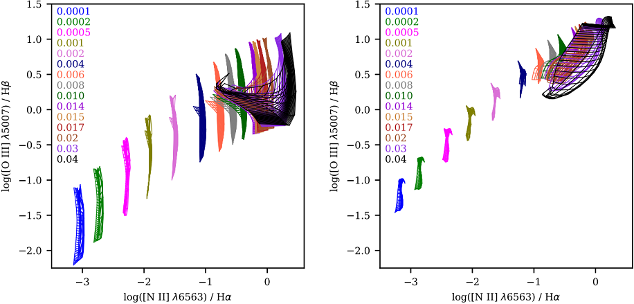
Fig. 6 Same diagrams as in Figure 2 except that the abundance sets are now from Gutkin et al. (2016). Shock velocities range from 100 to 1000km/s, and magnetic fields range from 0.0001 to 10 µG. The left panel corresponds to the line emission ratios from the shocked gas, while the right panel represents the line emission of both the shocked and precursor gas. The column in the upper left corner of each panel lists the mass fractions of each sequence of the corresponding color. The color figure can be viewed online.
TABLE 3 GRID SAMPLE OF THE LOW METALLICITY GRID DESCRIBED IN § 3.2
| Parameter | Sampled values |
|---|---|
| (C/O)/(C/O)⊙ | 0.26, 1.00 |
| Zism | 0.0001, 0.0002 0.0005, 0.001, 0.002, 0.004 |
| 0.006, 0.008, 0.010, 0.014, 0.01524, 0.017 | |
| 0.02, 0.03, 0.04 | |
| Vs (km s−1) | 100, 125, ..., 1000 |
| n0 (cm−3) | 1, 10, 102, 103, 104 |
| B0 (µG) | 10−4, 0.5, 1.0, 2.0, 3.23, 4.0, 5.0, 10 |
4.4. Grids of Truncated/Young Shock Models
The Allen et al. (2008) fast shock grid (§ 4.1) and the low metallicity shock grid (§ 4.3) contain models for which both the age of the shock was fixed prior to the calculations, by assuming arbitrary predetermined values. In certain cases, these parameters, when treated as free quantities, turn out to influence the line intensities in ways interesting to explore. In this section, we will indicate how the database can be used to explore the effect of the shock age on line ratios.
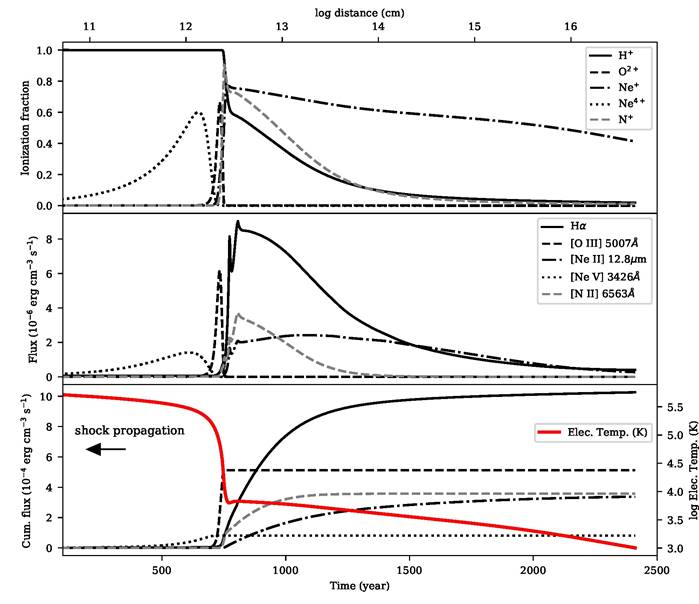
Fig. 7 Example of an ionization and emissivity structure for different elements at different ionization stages behind a 200 km s−1 shock propagating into a preshock density of 10 cm−3 and a transverse magnetic field of 1 µG with solar abundances. Top panel: Ionization fraction of HII, OIII, NeII and NeV. Middle panel: emissivity of Hα, [O III] 5007Å, [Ne II] 12.8µm, and [Ne V] 3426Å. Bottom panel: cumulative emissivity for the same ions as plotted in the middle panel. The shock front is propagating towards the left. The color figure can be viewed online.
The great majority of shock models found in the database are complete models, that is, they have been fully integrated until the shocked gas has cooled and fully recombined. They correspond to steady-state conditions; such shocks, with time, will slow down as they progressively convert their supersonic kinetic energy into radiative cooling. Although steady-state models can reproduce the conditions encountered in a wide variety of astrophysical objects, they are not always the optimal perspective. This is the case for instance for objects in which the shocks are relatively recent and therefore possess an incomplete cooling structure. For this particular case, a grid of incomplete cooling shock models, also known as truncated models or young shocks, is needed. Only a few calculations of young shocks can be found in the literature. They were computed to match individual object such as the Cygnus Loop filaments (Raymond et al. 1980; Contini & Shaviv 1982; Raymond et al. 1988), or low-excitation Herbig-Haro objects (Binette et al. 1985). The lack of grids including young/truncated shocks compelled us to add those to our database and to provide a way of exploring them.
Figure 8 illustrates the impact on the line ratios of using incomplete shocks. It can be compared to the similar Figure 6 of Kehrig et al. (2018). A very common assumption is that when one observes high values of [S II] or [N II] or [O II] lines when normalized to an H line, this implies the presence of shocks or, on the contrary, when these ratios turn out to be small, one often concludes that shocks cannot be involved in the gas excitation. Such generalized views must be applied with greater care. For instance, at low metallicities, we find that young shock models can easily fall under the classical Kewley curve (see Kewley et al. 2001).
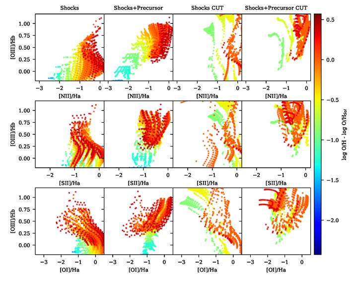
Fig. 8 Three classical BPT-type diagrams that compare complete with incomplete shock models (labeled “CUT”). All models were evaluated using a transversal magnetic field of 1 µG. The panels depict line ratios from either the shocked gas only or from both the shocked gas with the precursor emission. The color figure can be viewed online.
Truncated (or age-limited, or incomplete) shock models can be identified in the database using the cut keyword as a suffix at the end of the grid reference (ex: Allen08-cut, the only ones available for the moment). Before using any such model, it is important to be fully aware of what an incomplete or agelimited shock represents, which implies becoming familiar with the behavior of the ionization, temperature and line emissivities downstream from the shock front. To give an idea, Figure 7 shows how the evolution of these quantities is structured for a 200 km s−1 shock propagating into a gas with solar abundances and a preshock density of 10 cm−3. As this figure shows, the recombination occurs in stages, with the higher ionization species recombining towards lower values as time proceeds. The gas temperature shown in the bottom panel declines markedly with time. Both of these factors and the fact that the density increases as the temperature drops10 mean that the emissivity of any given line strongly varies with time along the cooling history of the postshock gas. The lower panel in Figure 7 shows how the cumulative (time-integrated) flux emission progresses, up to the desired final shock age. These time-integrated emission fluxes are actually stored in the database as a function of time. As revealed by the bottom panel, the line intensities are very sensitive to the time elapsed since the passage of the shock front. It is highly recommended to explore how such variations of the line intensities come about, and from there select the appropriate parameters to vary.
There are alternative parameters that can be used to specify the degree of shock completeness. The first is obviously the time elapsed (age) since the shock front initiated. The age parameter is located in the shockparams table in column named time, which is expressed in seconds. There is also the distance between the shock front and the final thickness of the shocked gas (at the specified shock age). This parameter is similarly located in the shockparams table in the column named distance, which is expressed in cm. Finally, there is the integrated column density of each ionic specie of the gas swept by the shock front until the gas has cooled and recombined (column named coldens), which is expressed in cm−2. The total H column density can be found with the following summation : N H = N HI +N HII . Complementary evaluations of how a specific line emissivity varies with age or depth requires knowing the integrated column density of the ion involved, which can be found in the ioncoldens table.
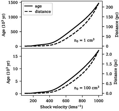
Fig. 9 Age and thickness of two shocks of different velocities that propagate in a gas cloud of density of either 1 cm−3 (top panel) or 100 cm−3 gas (bottom panel), assuming in both cases solar abundances and B 0 = 1 µG.
Both the distance travelled by the shock wave or, alternatively, its cumulative age can vary greatly depending on the initial shock conditions, as shown in Figure 9. An easy mistake a user can make is to define diagnostic diagrams such as those presented in Figures reffig:BPTAllen and 6 and superpose them to observations characterized by ages and/or sizes that are inconsistent with those of the models. This can be avoided by varying the preshock density until its thickness fits the desired scale. In the case of a complete shock model (without an external photoionization source), the final thickness and the time spent in cooling both scale as n − 0 1 (as seen in Figure 9).
Another potential mistake would be to use too high a preshock density, resulting in models where the density infered from its [S II] (λ6716Å/λ6731Å) doublet ratio (or its [O II] (λ3726Å/λ3729Å) doublet ratio) would be much higher than the density values derived from the observations. Consider, for instance, that a postshock temperature of 10 5.3 K without magnetic field will result in a [S II] doublet ratio corresponding to a density as high as ≈ 100n 0. The reason is that the density increases isobarically as the shock cools and, for the B = 0 case, the local density across the whole shock structure grows as the ratio T post /T e where T post and T e are the postshock and the local electronic temperature, respectively.
5. FUTURE EVOLUTION OF THE DATABASE
New models will be added depending on the research necessities of the authors of this paper or upon request by anybody interested in models that have not yet been included. As the web page is dynamic and will instantly reflect the current status of the database and of its model grids, any new references or model inclusions will be easily noticed. The authors of this paper will also do their best to update the 3MdBs grid of models as soon as possible after a new version of mappingsis available.
6. CONCLUDING REMARKS
In this paper, we presented an extension to the Mexican Million models database (3MdB) (Morisset et al. 2015), which comprises of the addition of shock models to the database. Important information was presented in this paper and the following is a list that summarizes the main points:
All shock models in the database were computedusing the shock modelling code mappingsv.
The database structure was explained in detailand information about how to connect and interact with the database was given. A website was created in order to follow the evolution of the database as new grids are added in the future.
At the time of publication, 3 grids are available. (1) The grid of Allen et al. (2008) was recomputed using mappingsv. (2) We extended the grids of Allen et al. (2008) to low metallicity using the abundances derived by Gutkin et al. (2016). (3) Grids of truncated/young shock models were computed.

