


 nueva página del texto (beta)
 Inglés (pdf)
 Artículo en XML
 Referencias del artículo
 Enviar artículo por email
 Citado por SciELO
  Similares en
SciELO
Similares en
SciELO 
 Permalink
1. INTRODUCTION
The galactic halo has plenty of astrophysical systems evolving under the interaction of the different galactic components. These substructures have diverse nature, dynamics and origins and together constitute the building blocks of the ongoing galaxy formation process. Among others, there are many stellar subsystems, such as the open and globular clusters (Binney & Tremaine 2008), pure gaseous ones, such as high velocity clouds (HVC) (Wakker & van Woerden 1997) and combined gaseous and stellar systems such as tidal streams and satellite galaxies (Ibata et al. 2001).
Open and globular clusters are segregated by several characteristics. Open clusters are considered to be younger and metal richer than their globular counterparts. In addition, open clusters are associated spatially with the galactic disc, while globulars are mostly distributed spherically in the halo. This segregation suggests that their formation processes are diverse. On one hand, the formation of open clusters is considered to be well understood as a result of the collapse and fragmentation of molecular clouds in the galactic disk (Elmegreen & Efremov 1997). The case of globular clusters exhibits a greater degree of complexity because, actually, there are two subpopulations of them. There is a metal poor globular cluster population (MPGC) extended across the halo, and a young, metal rich population (MRGC) (Carroll & Ostlie 2006). In addition, there are several cases that do not fit very well in the two previous subpopulations, as it is the case of the globular cluster ω Centauri (henceforth ω Cen) mainly due to its unusual size and metallicity dispersion (Harris 1999). This variety suggests that even considering only the globular clusters there are diverse formation mechanisms.
Different models have been proposed to explain the formation of the two subpopulations of globular clusters in the Galaxy. For the old MPGC subpopulation the widely accepted hypothesis is that they come from primordial density fluctuations in the density field at very high redshift, when the universe expanded and cooled to a temperature of about 4000 K and the baryonic density was approximately 104 atoms cm−3 (Reina-Campos et al. 2019). Under these conditions, the only density fluctuations that can grow with time have wavelength in excess of the critical Jeans length of about 5 pc (Peebles & Dicke 1968).
For the young MRGC subpopulation, it appears that there is not a single mechanism that can form all existing MRGC in a given galaxy (Ashman & Zepf 1992; Bekki & Freeman 2003; Shapiro, et al. 2010). One of the models suggests that a significant fraction of the metal-rich subpopulation may have originated in interacting galaxies, both minor and major mergers (Ashman & Zepf 1992). Major mergers cause several starburst episodes in the gaseous component of each galaxy, and globular clusters can be formed in regions with high gas density (Li et al. 2004). Minor mergers may also contribute to the young population with clusters formed within the small satellite galaxy from the interaction with the larger galaxy (Zepf & Ashman 1993). Also, the globular cluster system of the minor galaxy would eventually be accreted by the largest galaxy, also contributing to the MPGCs subpopulation (Forbes & Bridges 2010). The minor merger scenario can be seen in the Magellanic Clouds, where there is observational evidence of ongoing cluster formation and of an ancient cluster system bound to the clouds (Harris 1998; Georgiev et al. 2010). It was further suggested that the very central region of a satellite galaxy could form a globular cluster as the bound structure surviving the effects of the tidal stripping induced by its host galaxy (Bekki & Chiba 2002).
Moreover, recent observational evidence that suggests that several (if not all) GCs contain various stellar populations has come to light. For example, many GC stars have the same amount of Fe (and other heavy elements) inside a specific radius, but a wide variation in light elemental abundance (Li-Al) on a star-to-star basis (Conroy et al. 2011). Norris & Kannapan (2011) in a crucial study on this problem showed that some ultra-compact dwarf galaxies have color magnitude diagrams indistinguishable from those of GCs and the nuclei of dwarf galaxies. Bekki & Freeman (2003) found that the multiple stellar populations of ω Cen can be explained in terms of a nucleated dwarf galaxy scenario: the tidal field of the host galaxy induces gas inflow towards the center of the cluster progenitor, triggering multiple star bursts that lead to chemical enrichment. Other GC candidates that are thought to have formed in ostensibly dark matter potential wells deep enough to retain self-enriched Fe produced by supernovae Ia explosions include M22, NGC 1851 and Andromeda’s G1. The evidence showing chemical complexity of the cluster stellar populations suggests that the classical picture of all GC’s belonging to a single monolithic population should be reevaluated.
Similarly, HVCs appear to be the result of two possible mechanisms: One is the return to the disc of gas and dust expelled via supernovae events and the other is the infall of gas and dust from stripped subsystems, such as globular clusters or satellite galaxies (Wakker & van Woerden 1997).
A combination of both processes is necessary to explain the current distribution of high and intermediate velocity clouds. For example, from hydrodynamical simulations it is concluded that most massive HVC, such as the well known Complex C, were originated from ejection of material from the Milky Way’s disc (Fraternali et al. 2015); but the velocity dispersion, the metallicity, sizes and masses of the smallest clouds are consistent with an extragalactic origin (Blitz et al. 1999; Binney et al. 2009).
As a result of the tidal disruption of the Galaxy subsystems, the so-called tidal streams are originated. They are composed in most cases by stars and gas (Belokurov et al. 2006), like the Magellanic Stream, where recent observations have confirmed the presence of a young open star cluster most likely formed in the stream (Price-Whelan et al. 2018). Remarkably, all the streams observed in the Milky Way galaxy are clearly inhomogeneous and exhibit overdensities (Küpper et al. 2012). These overdensities evolve in the galactic potential as well, undergoing different processes that could eventually transform them into self gravitating systems like clusters. The main purpose of this work is to determine through N−body simulations of galaxy minor mergers if the overdensities in the tidal streams could really meet the conditions to be considered self-gravitating substructures. In a future work, we will investigate under what conditions the evolution of such substructures could lead to the formation of real astrophysical systems, such as globular clusters and high velocity clouds.
This paper is organised as follows: In § 2 we describe the setup of the N−body simulations, from the determination of the satellite galaxy initial position to the structure of the host galaxy passing through the astrophysical characteristics of the satellite. In § 3 we describe the analysis performed to the simulation outputs in order to search and characterise the overdensities. In § 4 we present our results. We finally discuss them and present the conclusions in § 5.
2. NUMERICAL PROCEDURES
The numerical setup of the N− body simulations used in this work comprises two stages. In the first stage the galaxies are generated in isolation. In this case, we generate a host disc galaxy and a spheroidal satellite galaxy, both with and without gas. We use these galaxy models to explore different merger configurations. In the following sections we describe in detail each part of the procedure.
We used the code Gadget2 to run all our simulations (details of the code can be found in Springel 2005). Gadget2 is a general purpose code to study the evolution of collisionless gravitational systems. Collisionless particles representing stars and dark matter evolve only under gravity using a tree method. To follow the evolution of gas an entropy based smoothed particle hydrodynamics (SPH) scheme (Springel & Hernquist 2002) is used with adaptive smoothing lengths, allowing conservation of energy and entropy in adiabatic regions. A synchronization scheme within the integration scheme is used; this is a quasi-symplectic KDK leap-frog with adaptive individual time-steps. The code uses a parallelization algorithm based on a space-filling curve to achieve high flexibility with high accuracy in tree force estimation.
2.1. Initial Conditions
2.1.1 Isolated Galaxies
The host galaxy in this work consists of a disk galaxy composed of a stellar disk and a dark matter halo. Neither gas in the disk nor a central spheroid are included in the model. The satellite galaxy is modelled as a spherical galaxy with a collisionless spheroid hosting a gaseous sphere in hidrostatic equilibrium. Initial conditions are computed using moments of the collisionless Boltzmann equation (Hernquist 1993; Springel et al. 2004). The dark matter halo of both galaxies follows a Hernquist density profile with scale length parameter adjusted to fit the shape of the NFW density profile, as done in Springel (2005).
Masses for the galaxies are taken from the CLUES simulations (Gottloeber et al. 2010; Forero-Romero et al. 2011). The mass of the dark matter halo hosting the disk galaxy is 7.9×10¹¹ h −1 M⊙ with a concentration parameter of c = 4.15. The satellite galaxy has a total mass of 3.2 × 10¹⁰ h −1 M⊙, and c = 4.26. Since it is not reasonable to simulate the formation of globular clusters observed today using properties of current host galaxies, the masses and properties of these two progenitor galaxies are related to the properties of the Milky Way galaxy and one of its satellites at z = 2, as observed from the constrained simulations made by CLUES. Galaxy disk structure (disk scale length, etc.) is modelled using the prescription of Mo et al. (1998), from which the scale parameters of the disk are r d = 1.53 kpc and z0 = 0.31 kpc.
The host galaxy has a stellar disk with a mass of 3.3 × 10⁹ h −1 M⊙, where we have used Moster et al. (2001) to estimate the total stellar mass for the given dark matter halo at z = 2 and assumed that all the stellar mass is deposited in the disk. Since we are not interested in the evolution of the gas in the disk of the host galaxy and we assume it does not have a dominant effect on the dynamics of the merger, we do not include a gaseous component in this galaxy.
The satellite galaxy is composed of collisionless particles representing dark matter or stars, and has also a gaseous component. Initially, the gas follows a density profile similar to the profile of the dark matter halo in hydrostatic equilibrium. Hydrostatic equilibrium is guaranteed through a gas temperature computed as Mastropietro et al. (2005)
where m p is the proton mass, k B is the Boltzmann constant and ρ g (r) is the gas mass density. In order to provide a favorable scenario for the formation of clusters from the material deposited in the stream, the total gas mass of the satellite has been chosen to be ≈ 16% of its total mass, providing the scenario for a gas rich merger. Although arbitrary, the gas fraction is in no way larger than the cosmological baryon fraction in a dark matter halo (Lin, et al. 2008). We could have included a disk of cold gas in the satellite; however, this would have implied a new degree of freedom in our simulations (see next section). Since the direction of the disk may affect the formation of a stream and the formation of potential candidates to GCs in our simulations, we decided to adopt a simpler spherical distribution looking for a solution general enough to study the formation of potential GCs in our simulations. We claim that if any structures are formed with this setup, for sure they can be formed in more favorable conditions where a disk provides cold gas to the stream.
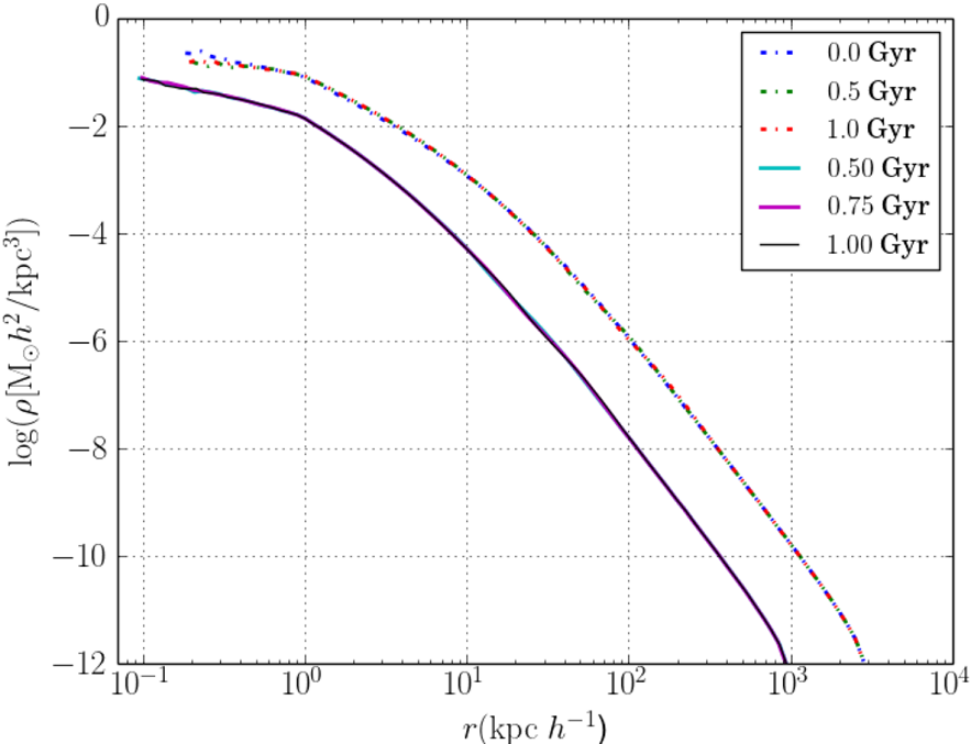
All galaxies are simulated in isolation after the generation of initial conditions in order to allow for numerical relaxation of the initial conditions. Figure 1 shows, for the dark matter halos, the convergence of the profiles from the initial conditions to the final relaxed density profiles. Note that the mass distribution only changes in the very inner region, and that after the first 1 Gyr the profile is relaxed. Also, the satellite galaxy reaches relaxation basically very close to the beginning. This check is relevant since it is important to make sure that there is no numerical artificial evolution on the density distribution of the galaxies, since in this way we can ensure that any change in the mass distribution of the system during the merger is due to the dynamics of the merger and is not spurious numerical noise or an instability originated from the initial conditions.
2.1.2. Merger Configuration
The mergers we plan to study in this work are somehow artificial in the sense that they do not correspond to any realistic system. However these simulations must reproduce the reality of our universe. In that sense, there is an infinite set of possible merger simulations we could run, each with a different orbit. To avoid running many orbits, and at the same time to try to reproduce the expected results from our understanding of the universe, we will use the results shown in Wetzel (2011) to choose the orbits to be studied in this work. In their work Wetzel (2011) study the probability distribution of orbital parameters of infalling satellite galaxies. From them, we use the mean orbital parameters as those of a representative merger that is in agreement with the current cosmological paradigm.
Then, to configure the merger we need to obtain realistic values of the initial position r 0 and velocity v 0 of the satellite galaxy. For that, from Wetzel (2011), we use the circularity η and the pericenter r p distance, which depend on the host halo mass Mhost and redshift z, and which for our host halo mass are distributed at the moment of their passage through the host’s virial radius according to the distribution functions shown in Figures 2 and 3. In both figures, the mean values of the circularity and the pericentre at z = 2 are highlighted with a small vertical green line.
TABLE 1 SPECIFICATIONS OF THE SATELLITE’S INITIAL ORBITAL CONFIGURATIONS CHOSEN FOR EACH SIMULATION*
| Name | Nomenclature | r0 (kpc) | v0(km/s) |
|---|---|---|---|
| Perpendicular | p | (0,0,198.34) | (0,34.9,0) |
| Planar Corotating | pcr | (0,198.34,0) | (-34.9,0,0) |
| Planar Contrarotating | pct | (0,198.34,0) | (34.9,0,0) |
| Inclined Corotating | icr | (99.6,99.6,140.25) | (-24.67,24.67,0) |
| Inclined Contrarotating | ict | (99.6,99.6,140.25) | (24.67,-24.67,0) |
*For a schematic view of each configuration, see Figure 4.
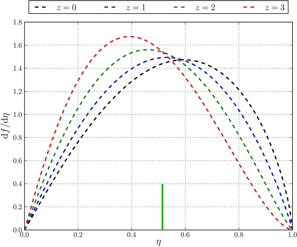
Fig. 2 Circularity distribution for the infalling satellites at different redshifts. The small vertical line indicates the average circularity at z = 2. The color figure can be viewed online.
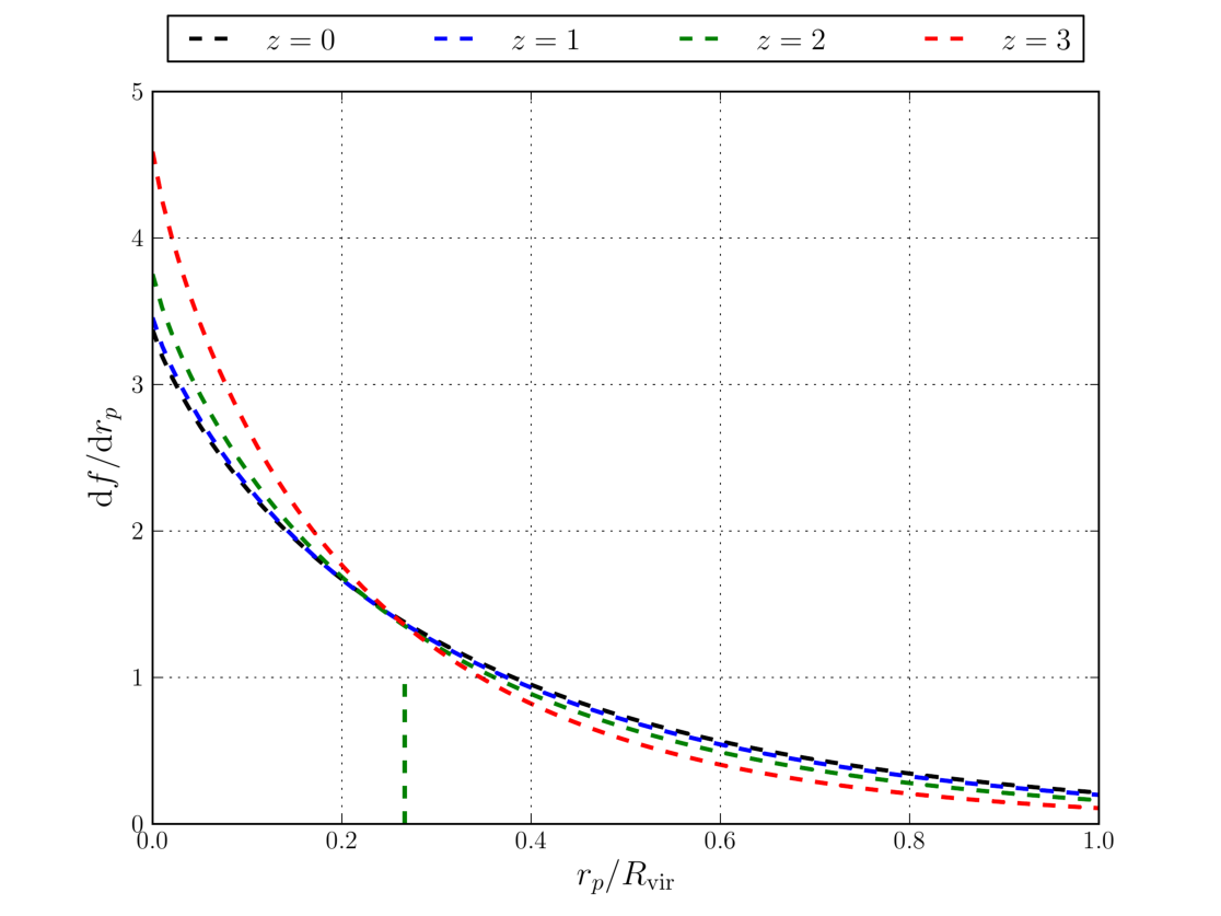
Fig. 3 Pericentre distribution for the infalling satellites; the redshift dependence is explicitly noted. The small vertical line indicates the average pericentric distance value at z = 2. The color figure can be viewed online.

Fig. 4 Schematic representation of the initial orbital configurations for the original five simulations. The host disc is rotating counterclockwise in the x-y plane.
Orbit circularity has a nearly constant small rate of decrease with redshift, while pericenter distance exhibits a decrease in its average values with
For our system, the numerical values were found to be e = 0.84 and r a = 198.34 kpc. Finally, making use of the vis-viva equation, the velocity at apogalacticon is simply
which turns to be 34.9 km/s for our infalling satellite.
In all simulations the host galaxy disk was always in the x−y plane with its angular momentum aligned with the z-axis. Based on the orbital parameters given in the previous paragraph, the merger was disposed in five different configurations. The only difference between each configuration is their location relative to the disc plane and its orbital motion direction relative to the disc rotation. The configuration parameters are shown in Table 1 and a schematic illustration of all of them is represented in Figure 4.
2.2. Simulations
Some of our simulations include star formation modeled as shown in Springel & Hernquist (2003). In this model a cold gas particle (cloud) is able to convert part of its mass into stars when several criteria are met. Its temperature should be lower than 104 K and its density should be larger than a predefined threshold density (ρth). Additionally, the cooling time should be shorter than the collapse time of the cloud
As it is well known, SPH suffers from fragmentation instabilities that lead small gas clumps to cluster, forming a set of non-physical structures (Bate & Burkert 1997; Torrey et al. 2013). Since what we are looking for in our simulations is exactly fluctuations in the mass distribution we need to make sure that we find candidates that are not just spurious numerical fragments formed due to the SPH instability. In order to avoid this, we ran the same set of initial conditions for several different particle resolutions and we found that the substructures present in the lower resolution simulation were recognizable in the higher resolution simulations, maybe with a little spatial displacement due to changes in the global dynamics of the system, as it can be seen in Figure 13 (In § 3.2 we show how these substructures were identified). Increasing the resolution of the simulations allows us to verify that what we find as substructure candidates are true candidates and not numerical artifacts. § 3.3 describes in better detail the results of our convergence study.

Fig. 5 Density values for the particles in GAS2 p−simulation against the identification particle number. This plot correspond to the snapshot at 3.75 Gyr after simulation starts. Density units are 1010 M⊙ /kpc3. The color figure can be viewed online.
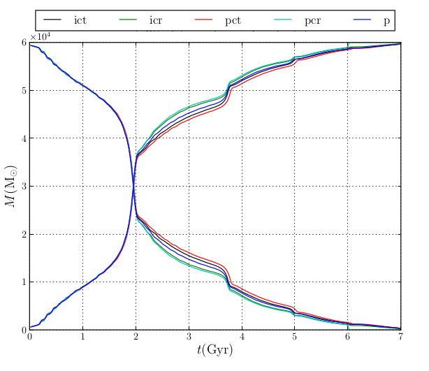
Fig. 6 Mass stripped from the satellite galaxy as a function of simulation time represented by the descending curves for each orbital configuration. The mass gained by the stream for each orbital configuration is shown by the ascending curves. The color figure can be viewed online.
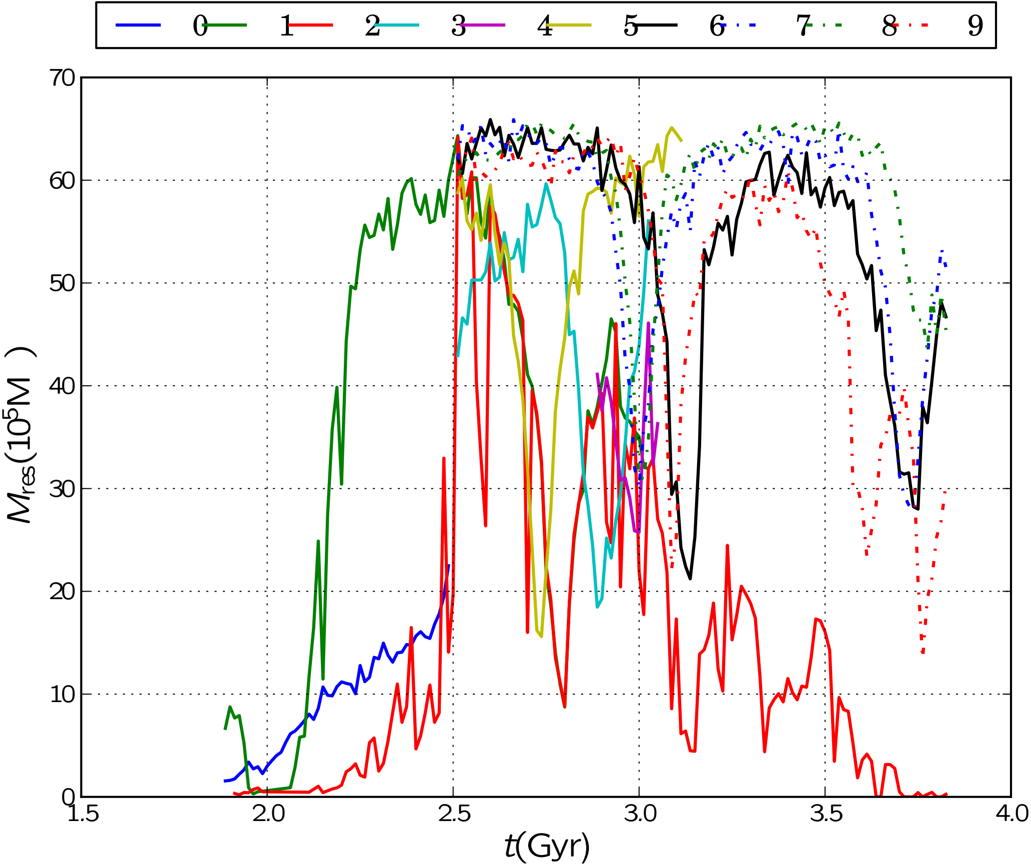
Fig. 7 Minimum resolvable masses for the nine candidates in GAS3 (equation 6). The minimum mass remain much smaller than the candidates total mass, see Figure 9. The color figure can be viewed online.
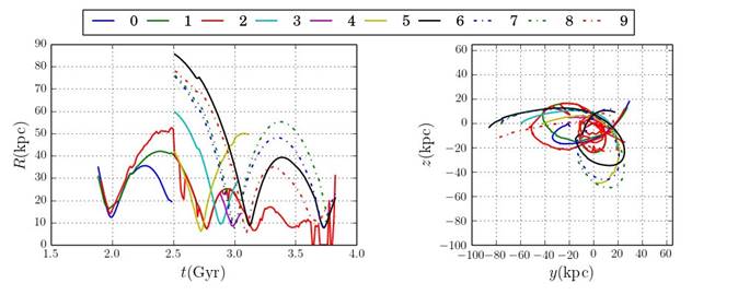
Fig. 8 Orbital structure of the nine candidates identified in GAS3. Left panel, Magnitude of the galactocentric vector position as a function of time. Right panel, Projection of the orbits in the y − z plane. The color figure can be viewed online.
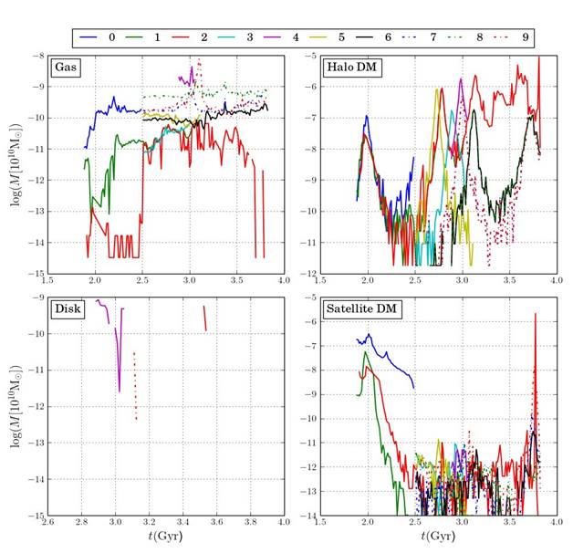
Fig. 9 Mass as a function of time for each candidate, segregated by type. The color figure can be viewed online.

Fig. 10 Top Panels: Real space projection on the z −y plane density-coded for the DMO2 simulation. Bottom Panels: Phase space projection on the r −v r plane with same density code. The density contrast is high in the elongated radial structures found in the tidal tails, but still does not exhibit the morphology of globular clusters. Panels on the left correspond to a time of 6.0 Gyr, right panels to 7.0 Gyr. Color values correspond to number density of points in log scale. The color figure can be viewed online.
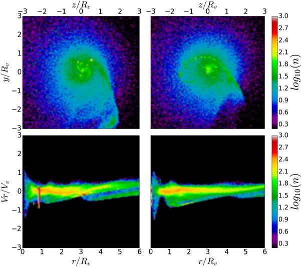
Fig. 11 Top Panels: Real space projection on the z − y plane coded with density. Bottom Panels: Phase space projection on the r−v r plane with same density code. R and V are the virial radius and velocity, respectively. A couple of snapshots of GAS2 are shown. The left panels correspond to a time of 5.00 Gyr, the right panels to 6.25 Gyr. Color values correspond to number density of points in log scale. The color figure can be viewed online.

Fig. 12 Top Panels: Real space projection on the z − y mapped with density. Bottom Panels: Phase space projection on the r−v r plane with same density color code. This plot is exactly Figure 10 but zooming to the internal region near the galactic disc for GAS2. Panels at the left correspond to a time of 5.00 Gyr while panels at the right are at 6.25 Gyr. Color values correspond to number density of points in log scale. The color figure can be viewed online.

Fig. 13 Candidates identified with the algorithm described in § 3.2. The number of clumps increases with increasing resolution. All plots correspond to a 3 Gyr simulation time. Top row, shows the candidates in GAS1. Middle row, candidates in GAS2. Bottom row, candidates in GAS3. In each row, at the left, the disc is seen face on, and at the right, the disc is seen edge on. The color figure can be viewed online.
We design two sets of experiments to explore the formation of substructures in the tidal streams of the satellite galaxy. The first consists in pure collisionless systems, or in other words, gas-free simulations. The main purpose of this first experiment is to verify if the collisionless matter alone could cluster and form bound systems without the influence of gas. This set of simulations was named DMO (Dark Matter Only), specifically DMO1 and DMO2 whose only difference is the number of particles in the satellite. In Table 2 we show the masses, number of particles and mass per particle of each galactic component in our models.
TABLE 2 COLLISIONLESS AND COLLISIONAL SIMULATIONS DATA*
| COLLISIONLESS SIMULATIONS | ||||
|---|---|---|---|---|
| Name | Component | Mass ( |
|
|
| DMO1 | Satellite |
|
|
|
| Disk |
|
|
|
|
| Halo |
|
|
|
|
| DMO2 | Satellite |
|
|
|
| Disk |
|
|
|
|
| Halo |
|
|
|
|
| COLLISIONAL SIMULATIONS | ||||
| GAS1 | Satellite |
|
|
|
| Gas |
|
|
|
|
| Disk |
|
|
|
|
| Halo |
|
|
|
|
| GAS2 | Satellite |
|
|
|
| Gas |
|
|
|
|
| Disk |
|
|
|
|
| Halo |
|
|
|
|
| GAS3 | Satellite |
|
|
|
| Gas |
|
|
|
|
| Disk |
|
|
|
|
| Halo |
|
|
|
|
*Np and mp are the number of particles and mass per particle, respectively.
The second set of simulations includes gas in the satellite and are designated as GAS. The difference among them is the increased resolution, GAS3 being the one with the highest resolution. Table 2 summarizes the resolution specifications of the GAS experiment.
As can be seen in Table 2, the SPH particle mass is of the order of 5 × 10³ h −1 M⊙ for GAS3. If we assume that typical masses for globular cluster candidates are of the order of 105 to 107 h −1 M⊙ in this simulation we can resolve globular cluster like structures with 20 to 2000 gas particles. Again, we are not interested to study star formation in those objects (which will imply the necessity of larger resolution simulations in order to properly sample star formation inside the clusters) but only to study study the collapse of gas in the candidate structures. Therefore, these numbers are good enough for the purposes of our work. We ran our simulations for a time interval of the order of 7 Gyr, long enough to study the evolution of the satellite remnants as would be observed at present.
3. ANALYSIS
3.1. Density Estimation
Overdensities are, by definition, regions with a spatial mass density larger than that of its surroundings. Hence, the best way to identify them is by estimating the mass density in the body of the tidal streams. High density regions will be the best candidates to form autogravitating substructures. We use the EnBiD (Entropy Based Binary Decomposition) algorithm to calculate the density distribution in real and phase spaces (Sharma & Steinmetz 2006).
The EnBiD algorithm is sensitive to the spatial anisotropies of the mass distribution through the implementation of an anisotropic smoothing tensor. In this way, any density underestimation is prevented due to the ability of the method to use particles along a preferred direction, and not only spherically symmetric around the point of interest, as the isotropic kernels do. Figure 5 shows the estimated density for the total number of particles in one of the GAS simulations at t = 3.75 Gyr. In the figure we show the density of gas, halo dark matter, disk and satellite particles. New stars formed from gas particles are also included. Note that this figure not only shows the densities of particles ranked by ID (and type) but allows to see the high density peaks. As we know, these density peaks are associated to gravitational instabilities and should be related to anisotropies in the density distribution of each galactic component. Therefore, an adequate density threshold can be selected to extract the prominent overdensities in the particle distribution.
As can be seen in the figure, the overal densities of the halo, disk and a fraction of particles of the satellite have a lower value than that for a fraction of particles of gas and stream material (which in this case corresponds to the last bump composed of satellite particles and new-born stars). The peaks in the values of the estimated density can be used to fix a density threshold ρ th that can serve to identify global overdensities, as shown by the horizontal line in Figure 5. Notice that only a fraction of gas, satellite and new star particles are above this threshold, and one expects that since those overdensities are induced by the gravitational instability, they would be spatially correlated, as can be seen in Figure 13. This density threshold is an important part of the process of identification of high density peaks corresponding to the seed of the identification of potential cluster candidates.
3.2. Identification of Substructure Candidates
Once the densities of the particles have been calculated, we aim to identify the overdensities in the field of the stream in order to label them as possible candidates. We start by estimating density maps as described in the previous section. These maps highlight the overdensities above the underlying distribution of particles, as shown in Figures 10 and 11. Then, the identification is carried out by the following series of steps:
First the candidates are identified by performing a selection of particles through a phase space density threshold ρth. Particles with phasespace densities below the density threshold are ruled out as potential center of some candidate clump. The value of ρth was chosen examining the values of the density of the simulation using, for instance, a plot like the one shown in Figure 5, in which we clearly distinguish between particles of high and low density. The density threshold could be different from one simulation to another.
Once the particles with ρ < ρth are ruled out, we construct a three dimensional spatial plot of the particles that are left. In this plot, we identify, by eye a centre of each overdensity. The coordinates of the centre at that particular snapshot are then estimated to be r c = (x c ,y c ,z c ). For this we choose a random snapshot, but it is preferable for the system to be sufficiently evolved, maybe after the satellite has passed several times through the disk. The fact that at this point we choose by eye the position of the candidate has no effect on the results. Using for example a method like spherical overdensity would work equally well, since we are just guessing the position of the overdensity.
Based on the three dimensional plot built before, the size of the overdensity can be roughly estimated. We assign a spherical radius
With the ID number of each particle in the candidate list, we track the position and velocities of such particles in all the snapshots of the simulations. At this point, we compute the center of mass of the particles in the candidate clump (for each snapshot) and look for particles of any kind that lie within a sphere of radius R th = 0.7kpc, including dark matter particles from the host and the satellite halos, gas and disk particles, and new stars born during the interaction. Notice that across the snapshots particles can come in and out of the sphere of R th = 0.7kpc, meaning that the list of particles that actually belong to the candidate has to be updated dynamically.
Then, for every snapshot, we compute the properties of the clump in order to tie the evolution of the visually identified clouds to an astrophysical observed system. Such properties are center of mass, binding energy, total mass, mass by type of particle, central and mean densities, tidal and core radii, and the tidal heating.
3.3. Resolution Study Against Artificial Fragmentation
The numerical scheme used to simulate the hydrodynamics of the gas could impact the formation of clumps within the molecular clouds in an artificial way. The resolution of a SPH simulation involving gravity is therefore a critical quantity in order to obtain realistic results from physical process rather than artificially ones induced by numerical fluctuations.
As it is widely known, in SPH the properties of gas particles are obtained by summing the properties of all the particles that lie within a sphere with a radius known as the smoothing length h. The smoothing lengths are constrained to contain approximately a number of particles, called number of neighbours Nngb, in the sphere of radius h. Since the gravitational softening is set equal to h, the mass contained in the sphere cannot be roughly equal to the local Jeans mass, otherwise the collapse would be inhibited by the softening of the gravitational forces.
Thus, the called minimum resolvable mass, Mres must always be less than the local Jeans mass M J given by
where ρ is the density of the gas at temperature T, k B is the Boltzmann constant, m H is the mass of
the hydrogen atom and µ is the gas mean molecular weight (Draine 2011). Taking Mres as the mass of 2Nngb particles, it can be estimated as (Bate & Burkert 1997):
where Mgas and Ngas are the total mass and particle number of the gas. The previous expression explicitly shows that for a larger number of particles, the minimum resolvable mass decreases and the collapse and fragmentation will be less affected for the numerical implementation.
The condition (6) with Nngb = 128 was tested for the clumps in the satellite galaxy gas that we selected as substructure candidates with the previous recipe. The strategy adopted for the identification of the progenitors and the results obtained of such strategy are depicted in the next sections.
Figure 7 shows the time evolution of the minimum resolvable mass for each cluster according to equation 6, which remains much smaller than the local Jeans mass.
4. RESULTS
In Figure 6 we show the mass stripped from the satellite galaxy as a function of simulation time. Each line in Figure 6 represents the evolution of the mass stripped from the satellite for each of the five orbital configurations presented in Table 1. As can be seen in the figure, the rate of mass loss is quite similar for every orbital configuration of the merger. For this reason, since in our experiments we found no reason to prefer any orbit over another on the basis of the amount of mass stripped of the satellite, we decided, without loss of generality, to run our high resolution simulations only for the orbit perpendicular to the plane of the galaxy.
As can be seen in the figure, there are breaks in the mass curve located at about 2, 3.8 and 5 Gyr. These breaks are associated with the periastron passages during the merger. Clearly, the first passage strips the largest amount of mass from the satellite. Most of the mass ejected during the first passage is gas that is heated up during the collision and should remain bounded to the host galaxy, potentially forming the overdensities that are interesting for our study.
Figure 10 shows the projected particle distribution of the DMO2 simulation at two different time snapshots, t = 6 Gyr and t = 7 Gyr. The figure shows (at the top, in color code) the density of the streams; the umbrella effects associated to the distribution of the merger remnant of a satellite interacting with a massive host galaxy can be seen. At the bottom, each figure shows the pseudo phase space diagrams; the disturbances in phase space associated to the structures of the streams and merger remnants can be seen. As shown at the two different time snaps, there is a diffuse structure that appears at time 6 Gyr (in real space and in phase-space) but after 1 Gyr it is already washed out. This happens to all structures observed in the simulations with only collisionless matter.
Figure 11 shows the same projected particle distribution coded in Figure 10 but for the GAS2 simulation. Unlike the previous case, it is clear from the projected density and phase-space density that there are more overdensities, and that they survived for several orbital periods keeping their structure for a significant fraction of their lifetime. Figure 12 shows a zoom of the inner region of Figure 11 near the galactic disc. From this result, constrained by the resolution of our DMO simulations, we conclude that to form long lasting structures we need cold gas which helps to keep the particles gravitationally bound.
GAS simulations are thus the ones with better results for the formation of stream substructures. Consequently, we targeted them to apply the algorithm for identification of substructure candidates; results are shown in Figure 13, where the galactic disc of the host galaxy is also shown as a reference. The plots show the candidates identified in the simulations GAS1, GAS2 and GAS3, all for a simulation time of 3 Gyr. for comparison purposes. It is clear that among all the simulations of this work the higher resolution simulation has the greater number of substructures, which in turn, have the highest number of particles. For this reason we only study the properties of the substructures of GAS3.
For each substructure identified in the simulation we investigated several properties. In GAS3 we identified 10 overdensities associated to the 10 densest peaks, labeled with numbers 0 to 9; for each one we start by determining their orbital evolution. Figure 8(b) shows the y − z projection of the orbit of the center of mass followed by each candidate. Figure 8(a) shows the distance of each candidate to the center of the disk of the host galaxy as a function of time. The notable aspect of this plot is the fact that the candidates persist during a significant amount of time, with lifetimes of the order of 1 Gyr or longer.
Figure 9 shows the evolution of the mass content of each candidate in GAS3. For all the candidates, the principal constituent is gas. The high peaks of host dark matter content present in the candidates are circumstantial particles that are counted by the algorithm when the candidate traverses the central region of the dark halo where the density is sufficiently high to cause miscounting of host dark particles as candidate particles. The masses found for each candidate correspond to the masses measured for globular clusters and high-velocity clouds, both ranging from 103 M⊙ to a maximum of 106 M⊙ on average. However, there are several cases of clusters with masses over 106 M⊙ (Harris 1999; Wakker & van Woerden 1997).
4.1. Dark Matter in Cluster Candidates
The candidate labeled as Candidate 0 was the only one formed by gas and particles of another species. Figure 9(a) clearly shows that the predominant mass component is the dark matter of the satellite from where it comes. This dark matter component is not circumstantial, and is an important part of this candidate during its lifetime. The rest of the candidates are basically cores of gas, without dark matter or disc stars. This suggests that through this formation mechanism one could expect to find dark matter in globular cluster.
5. SUMMARY AND DISCUSSION
In this work we use N-body simulations of satellite galaxies undergoing minor merger with a larger host galaxy. Our goal is to find if there is formation of globular cluster-like systems in the tidal stream formed by the material stripped from the satellite. The work is divided in two main parts: The first part is performed to explore the possibility of formation of structures from pure collisionless simulations, the second part is dedicated to simulate the formation of cluster-like structures from mergers that included gas.
We performed several estimations in the simulations to identify the stream and the possible autogravitating substructures inside it. The approach adopted to identify substructures was the estimation of the phase-space density which reveals the presence of substructures as density peaks.
The density estimation clearly identifies overdensity regions in which a cluster-like structure could be formed. As a first conclusion we argue that without gas, the substructures that could be formed (if at all) have a short life time, as none of the overdensities show a definite morphology or stability over time. When gas is included, several clumps appear.
The results including gas physics are remarkably different. The candidates identified in the simulation proved to be real physical structures that live for a considerable amount of time and whose orbital evolution shows them to be objects in the surroundings of the galactic disk. The total absence of stars formed within the clumps is mainly due to the thermodynamic setup of the gas as an initially isothermal sphere; the temperature of the gas is high enough to inhibit instantaneous star formation in the candidates. Another factor at play is that the implementation/parameters of the feedback we used in the simulations, make the feedback too strong in the satellite galaxy. Oppenheimer & Davé (2006) discuss that the original implementation of Springel & Hernquist (2003) does not work equally well for all halo masses, and that the model and the parameters should be somehow mass dependent. As it was already mentioned, due to the physics involved in the problem of star formation in complex scenarios, it is beyond the scope of this work to study star formation in these candidate structures.
The main conclusion of this work is that substructures (globular clusters and high velocity clouds) could be formed in the tidal streams of gas rich satellites. The validity and scope of this main conclusion should be tested by running simulations with higher resolutions and taking in to account different feedback and star formation models. This is the road map for future work that will contribute to improve and supplement the results presented here.
Certainly our experiments are limited. First of all, we could study all other orbital configurations to complement the study. However, having found that one of the merger configurations already produced candidate clusters, the goals of our work were already meet. Studying under which conditions (merger orbits) it is easier to form this kind of structures is an interesting idea, but indeed it would require a larger amount of computing time in order to run a suite of simulations.
We could have included gas in the disk of the host galaxy; we could also have included a hot gas halo in the main galaxy; we did not do it because it made the simulations much more expensive. Indeed both aspects are important because these gaseous components could affect the dynamics of the merger and the dynamics of the gas in the stream through ram pressure stripping and shock heating. Both processes could work stripping more gaseous material from the satellite, thus increasing the amount of gas in the stream. We expect that this will contribute to increase the fraction of gas that could end up falling into cluster candidates. However the limited design of our experiment suffices to answer the question of the formation of candidate globular cluster structures by this kind of processes, and we expect that including other gaseous components will not change the main conclusions of the work.

