


 nueva página del texto (beta)
 Inglés (pdf)
 Artículo en XML
 Referencias del artículo
 Enviar artículo por email
 Citado por SciELO
  Similares en
SciELO
Similares en
SciELO 
 Permalink
1. INTRODUCTION
From recent observations of the European space mission Planck, the contribution of the baryonic matter to the total matter-energy density of the Universe was inferred to be only ≈ 5%, while the dark sector constitutes ≈ 95%, of which ≈ 26% is dark matter (DM) and ≈ 69% is dark energy (DE), or a positive cosmological constant Λ (Planck Collaboration et al. 2016). The observations of type Ia supernovae, the anisotropies observed in the cosmic microwave background, the acoustic oscillations in the baryonic matter, the power-law spectrum of galaxies, among others, represent strong evidences for the standard cosmological model, the so-called ΛCDM concordance model.
The DM component was postulated in order to explain the observed rotation curves of spiral galaxies, as well as the mass-to-light ratios in giant galaxies and clusters of galaxies (Zwicky 1933, 1937; Smith 1936; Rubin 1983), the observed gravitational lenses and the structure formation in the early Universe, among other astrophysical and cosmological phenomena (see e.g. Bertone et al. 2005; Bennett et al. 2013). On the other hand, the DE or Λ has been postulated in order to explain the accelerated expansion of the Universe (Perlmutter et al. 1999). The ΛCDM model fits quite well most of these observations. However, direct or indirect searches of candidates to DM have yielded null results. In addition, the lack of any further evidence for DE opens up the possibility to postulate that there are no dark entities in the Universe, but instead, the theory associated to these astrophysical and cosmological phenomena needs to be modified.
Current models of DM and DE are based on the assumption that Newtonian gravity and Einstein’s general relativity (GR) are valid at all scales. However, their validity has only been verified with highprecision for systems with mass to size ratios of the order or greater that those of the Solar System. In that sense, it is conceivable that both the accelerated expansion of the Universe and the stronger gravitational force required in different systems represent a change in our understanding of gravitational interactions.
Moreover, from the geometrical point of view, theories of modified gravity are viable alternatives to solve the astrophysical and cosmological problems that DM and DE are trying to solve (see e.g. Schimming & Schmidt 2004; Nojiri & Odintsov 2011a; Capozziello & Faraoni 2011; Nojiri et al. 2017). In this sense, any theory of modified gravity that attempts to supplant the DM of the Universe, must account for two crucial observations: the dynamics observed for massive particles and the observations of the deflection of light for massless particles.
The first non-relativistic modification, proposed to fit the rotation curves and the Tully-Fisher relation observed in galaxies, was the Modified Newtonian Dynamics (MOND) (Milgrom 1983b,a). Due to its phenomenological nature and its success in reproducing the rotation curves of disc galaxies (see Famaey & McGaugh 2012, for a review), it is understood that any fundamental theory of modified gravity should adapt to it on galactic scales in the low accelerations regime. However, from the study of groups and clusters of galaxies it has been shown that, even in the deep MOND regime, a dominant DM component is still required in these systems (60 to 80% of the dynamical or virial mass). The central region of galaxy clusters could be explained with a halo of neutrinos with 2 eV mass (which is about the upper experimental limit), but on the scale of groups of galaxies, the central contribution cannot be explained by a contribution of neutrinos with the same mass (Angus et al. 2008). Moreover, the Lagrangian formulation of MOND/AQUAL (Bekenstein & Milgrom 1984), is not able to reproduce the observed gravitational lensing for different systems (see e.g. Takahashi & Chiba 2007; Natarajan & Zhao 2008), mainly because it is not a relativistic theory and, as such, it cannot explain gravitational lensing and cosmological phenomena, which require a relativistic theory of gravity.
Through the years, there have been some attempts to find a correct relativistic extension of MOND. The first one was proposed by Bekenstein (2004), with a Tensor-Vector-Scalar (TeVeS) theory. This approach presents some cumbersome mathematical complications and it cannot reproduce crucial astrophysical phenomena (see e.g. Ferreras et al. 2009). Later, Bertolami et al. (2007) showed that for a particular generalization of the f(R) metric theories, with R the Ricci scalar, by coupling the f(R) function with the Lagrangian density of matter
In this article we focus on the f(χ) theories in the metric formalism, proposed in Bernal et al. (2011b), where the dimensionless Ricci scalar χ is constructed by introducing a fundamental constant of nature with dimensions of acceleration of order ≈ 10−10 m/s2. Through the inclusion of the mass of the system into the gravitational field’s action, the authors showed that the f(χ) = χ 3/2 metric theory is equivalent to the MONDian description in the non-relativistic limit for some systems, e.g. for those with spherical symmetry, but with remarkable advantages. From the second order perturbation analysis, this metric theory accounts in detail for two observational facts. First, it is possible to recover the phenomenology of flat rotation curves and the baryonic Tully-Fisher relation of galaxies, i.e. a MONDlike weak field limit. Second, this construction also reproduces the details of observations of gravitational lensing in individual, groups, and clusters of galaxies, without the need of any DM component (Mendoza et al. 2013). At the same second order also, the theory is coherent with a parametrized postNewtonian description (PPN) where the parameter γ = 1 (Mendoza & Olmo 2015).
The f(χ) metric theories are an extension of the f(R) metric gravity, which has been extensively studied as an alternative to DM and DE (see e.g. Sotiriou & Faraoni 2010; De Felice & Tsujikawa 2010; Capozziello & Faraoni 2011; Nojiri & Odintsov 2011a). In cosmology, it has been shown that f(R) metric theories can account for the accelerated expansion of the Universe, as well as for an inflationary era, e.g. for f(R) = R+αR 2 (Starobinsky 1980), where α is a coupling constant. Moreover, there are models for unification of DE and inflation, or DE and DM (see e.g. Nojiri & Odintsov 2011; Nojiri et al. 2017).
As shown in Carranza et al. (2013), an f(χ) description of gravity can be understood as a particular F(R,T) theory (Harko et al. 2011), where the gravitational action is an arbitrary function of the Ricci scalar and the trace of the energy-momentum tensor T. Within the F(R,T) description, Harko et al. (2011) have shown that, through the choice of suitable F(T) functions, it is possible to obtain arbitrary FLRW universes, and that the model is equivalent to having an effective cosmological constant. For the particular f(χ) = χ 3/2 metric theory used here, Carranza et al. (2013) have shown that the model can fit data of type Ia supernovae with a dust FLRW Universe, showing that the accelerated expansion of the Universe at late times (χ ≈ 1) could be explained by an extended theory of gravity deviating from GR at cosmological scales.
In general, both descriptions result in field equations that depend on the mass of the source, except for the particular case f(χ) = χ, where GR is recovered. This scenario presents even more richness than standard f(R) theories, because of the matter-geometry coupling, since it is possible to reconstruct diverse cosmological evolution by choosing different functions for the trace of the stress-energy tensor. Further research on the cosmological implications of f(χ) theories must be done in order to accept or discard models trying to replace the DM, or the DM and the DE of the Universe.
In the present work, we extend the perturbation analysis developed in Mendoza et al. (2013) for f(χ) = χ 3/2 in the metric formalism in powers of v/c (where v is the velocity of the components of the system and c is the speed of light), up to the fourth order of the theory, and focus on applications to clusters of galaxies. As shown in Sadeh et al. (2015) and first hypothesized in Wojtak et al. (2011), there exist observational relativistic effects of the velocity of galaxies at the edge of galaxy clusters, showing a difference of the inferred background potential with the galaxy’s inferred potential. With this motivation in mind, we have calculated the fourth order relativistic corrections and shown that they can fit the observations of the dynamical masses of 12 Chandra X-ray clusters of galaxies from Vikhlinin et al. (2006).
The article is organized as follows: In § 2, the weak field limit for a static spherically symmetric metric of any theory of gravity is established and we define the orders of perturbation to be used throughout the article. In § 3, we show the particular metric theory to be tested with astronomical observations. The results from the perturbation theory for the vacuum field equations, up to the fourth order in perturbations, are presented. With these results, we obtain the gravitational acceleration generated by a point-mass source and its generalization to extended systems, particularly for applications to clusters of galaxies. In § 6, we establish the calibration method to fit the free parameters for the metric coefficients, from the observations of the dynamical masses of 12 Chandra X-ray clusters of galaxies. Finally, in § 7, we show the results and the discussion.
2. PERTURBATIONS IN SPHERICAL SYMMETRY
In this section, we define the relevant properties of the perturbation analysis for applications to any relativistic theory of gravity. Einstein’s summation convention over repeated indices is used. Greek indices take values 0,1,2,3 and Latin ones 1,2,3. In spherical coordinates (x 0 ,x 1 ,x 2 ,x 3) = (ct,r,θ,ϕ), with t the time coordinate and r the radial one, θ and ϕ the polar and azimuthal angles respectively; the angular displacement is dΩ2 := dθ 2 +sin2 θ dϕ 2. We use a (+,−,−,−) signature for the metric of the space-time.
Let us consider a fixed point-mass M at the center of coordinates; in this case, the static, spherically symmetric metric g µν is generated by the interval
where, due to the symmetry of the problem, the unknown functions g 00 and g 11 are functions of the radial coordinate r only.
The geodesic equations are given by
where Γ α µν are the Christoffel symbols. In the weak field limit, when the speed of light c → ∞, ds = c dt, and since the velocity v ≪ c, then each component v i ≪ dx 0 /dt, with v i := (dr/dt, r dθ/dt, r sinθ dϕ/dt). In this case, the radial component of the geodesic equations (2), for the interval (1), is given by
where the subscript ( ) ,r := d/dr denotes the derivative with respect to the radial coordinate r. In this limit, a particle bounded to a circular orbit around the mass M experiences the radial acceleration given by equation (3), such that
for a circular or tangential velocity v. At this point, it is important to note that the last equation is a general kinematic relation, and does not introduce any particular assumption about the specific gravitational theory. In other words, it is completely independent of the field equations associated to the structure of space-time produced by the energymomentum tensor.
In the weak field limit of the theory, the metric coefficients take the following form (see e.g. Landau & Lifshitz 1975):
for the Newtonian gravitational potential ϕ and an extra gravitational potential ψ. As extensively described in Will (1993, 2006), when working in the weak field limit of a relativistic theory of gravity, the dynamics of massive particles determines the functional form of the time-time component g 00 of the metric, while the deflection of light determines the form of the radial g 11. At the weakest order of the theory, the motion of material particles is described by the potential ϕ, taking ψ = 0 (Landau & Lifshitz 1975). The motion of relativistic massless particles is described by taking into consideration not only the second order corrections to the potential ϕ, but also the same order in perturbations of the potential ψ (Will 1993).
For circular motion about a mass M in the weak field limit of the
theory, the equations of motion are obtained when the left-hand side of equation (3)
is of order v
2
/c
2 and when the right-hand side is of order ϕ/c
2. Both are orders
Now, the extended regions of clusters of galaxies need a huge amount of DM to explain
the observed velocity dispersions of stars and gas in those systems. In the outer
regions, the velocity dispersions are typically of order 10−4 −
10−3 times the speed of light. Hence, the Newtonian physics given by
an
In order to test a gravitational theory through different astrophysical observations (e.g. the motion of material particles, the bending of light-massless particles, etc.), the metric tensor g µν is expanded about the flat Minkowski metric η µν , for corrections h µν ≪ η µν , in the following way:
The metric g
µν
is approximated up to second perturbation order
In this paper, we develop perturbations of the relativistic extended model
f(χ) = χ
3/2
up to the fourth order in the time-time metric component,
In other words, the metric is written up to the fourth order in the time component and up to the second order in the radial one. The contravariant metric components of the previous set of equations are given by
3. EXTENDED F(χ) METRIC THEORIES
3.1. Field Equations
The f(χ) metric theories, proposed in Bernal et al. (2011b), are constructed through the inclusion of MOND’s acceleration scale a 0 (Milgrom 1983a,b) as a fundamental physical constant that has been shown to be of astrophysical and cosmological relevance (see e.g. Bernal et al. 2011a; Carranza et al. 2013; Mendoza et al. 2011; Mendoza 2012; Hernandez et al. 2010, 2012; Hernandez & Jiménez 2012; Mendoza et al. 2013; Mendoza & Olmo 2015; Mendoza 2015).
The action S f for metric theories of gravity, rewritten with correct dimensional quantities for a mass M generating the gravitational field, is given by (Bernal et al. 2011b)
where G represents Newton’s gravitational constant, for any arbitrary function f(χ) of the dimensionless Ricci scalar χ:
where L M is a length-scale depending on the gravitational radius r g and the mass-length scale l M of the system, given by (Mendoza et al. 2011)
with a 0 = 1.2×10⁻¹⁰ m/s2 the MOND’s acceleration constant (see e.g. Famaey & McGaugh 2012, and references therein) and ζ is a coupling constant of order one calibrated through astrophysical observations.
The matter action takes its ordinary form
with
Equation (11) is a particular case of a full gravityfield action formulation in which the details of the mass distribution appear inside the gravitational action through L M , except for f(χ) = χ, where the Hilbert-Einstein action is recovered. For the particular case of spherical symmetry, the mass inside action (11) becomes the mass of the central object generating the gravitational field. It is also expected that for systems with a high degree of symmetry, the mass M is related to the trace of the energymomentum tensor T through the standard definition
In what follows, we work with f(χ) theories in the metric formalism. Note that a metric-affine formalism can also be taken into account (see e.g. Barrientos & Mendoza 2016).
Now, the null variation of the complete action, i.e. δ (S f + S m) = 0, with respect to the metric tensor g µν , yields the following field equations:
where the prime denotes the derivative with respect to the argument, the Laplace-Beltrami operator is ∆ := ∇
µ
∇µ and the energy-momentum tensor T
µν
is defined through the standard relation δ
where R µν is the standard Ricci tensor. The trace of equations (17) is given by
where T := T α α .
Bernal et al. (2011b) and Mendoza et al. (2013) have shown that the function f(χ) must satisfy the following limits:
in order to recover Einstein’s GR in the limit χ ≫ 1 and a relativistic version of MOND in the regime χ ≪ 1.
Now, a complete extended cosmological model without the introduction of any DM and/or DE components should explain several cosmological observations, e.g. the cosmic microwave background, large scale structure formation, baryonic acoustic oscillations, etc. However, when mass-energy to scale ratios reach sufficiently large numbers, of the order or greater than the ones associated to the Solar System, then GR must be the correct theory to describe them. In this direction, Mendoza (2012) has proposed a “transition function” between both regimes, GR and “relativistic MOND”, to describe the complete cosmological evolution:
For this function, GR is recovered when χ ≫ 1 in the strong field regime and the relativistic version of MOND is recovered when χ ≪ 1 in the weak field limit. Some observations suggest an abrupt transition between both limits of function (20) (see Mendoza et al. 2013; Hernandez et al. 2013; Mendoza 2015), meaning that it might be possible to choose the following step function to describe the evolution of the Universe:
However, in this work we are interested in the regime where GR should be modified, which in our case corresponds to the relativistic regime of MOND, assuming that where GR works well there should not be a modification. Thus, in the following, we work in the limit χ ≪ 1 only.
Note that the “transition functions” (21) and (22) converge to GR at very early cosmic times, when inflation should dominate the behavior of the Universe. This can be thought of as a correct limit by including an inflaton field for the exponential expansion of the Universe, or one can think that at the very early epochs the f(χ) function should be proportional to the square of the Ricci scalar in such a way that a Starobinsky (1980) exponential expansion is reached (see also Nojiri et al. 2017).
3.2. Relativistic MOND (χ ≪ 1)
For the case χ ≪ 1, the first two terms on the left-hand side of equation (19) are much smaller than the third one, i.e. f ′(χ)χ−2f(χ) ≪ 3L 2 M ∆f ′(χ), at all orders of approximation (Bernal et al. 2011b). This fact means that the trace (19) can be written as
For the field produced by a point mass M, the righthand side of last equation (23) is null far from the source, and so the last relation in vacuum at all perturbation orders can be rewritten as
Now, as a simple case of study, we assume a power-law form for the function f(χ):
for a real power b. In this case, relation (24) is equivalent to
at all orders of approximation for a power-law function of the Ricci scalar
Substitution of function (25) into the null variations of the gravitational field’s action (11) in vacuum leads to
and so
From the last relation, we can see that the same field equations in vacuum are obtained for a powerlaw function (25) in the f(χ) theory, as well as for a standard power-law f(R) metric theory (27), but with the important restriction (26) needed to yield the correct relativistic extension of MOND (χ ≪ 1 limit). Mendoza et al. (2013) showed that this condition is crucial to describe the details observed for gravitational lensing for individuals, groups and clusters of galaxies, and differs from the results obtained in Capozziello et al. (2007), for a standard f(R) power-law description in vacuum. As discussed in Mendoza et al. (2013), such a discrepancy occurs from the sign convention used in the definition of the Riemann tensor, giving two different choices of signature that effectively bifurcate on the solution space, a property which does not appear in Einstein’s general relativity. This is due to higher order derivatives with respect to the metric tensor that appear in metric theories of gravity (cf. equations (17) and (19)). Following the results in Mendoza et al. (2013), we use the same definition of Riemann’s tensor sign and the branch of solutions that recover the correct weak field limit of the theory, in order to explain the rotation curves of spiral galaxies based on the Tully-Fisher relation, and the gravitational lensing observed at the outer regions of groups and clusters of galaxies, within the point-mass description.
Given the equivalence of the power-law f(χ) models with the standard f(R) metric theories, the standard perturbation analysis for f(R) theories constrained by equation (26) is developed for the power-law description of gravity (25) in the weak field limit, and for the first-order MOND-like relativistic correction in Mendoza et al. (2013). In this case, the standard field equations (17) reduce to (see e.g. Capozziello & Faraoni 2011)
where the fourth-order terms are grouped into Hµν := −(∇µ∇ν − g µν ∆)f ′(R). The trace of equation (30) is given by
with H := Hµνg µν = 3∆f ′(R).
For the case of the static spherically symmetric space-time (1), it follows that
and the trace
4. PERTURBATION THEORY
In this subsection, we present the perturbation analysis for f(χ) metric theories. Perturbations applied to metric theories of gravity, including GR, are extensively detailed in the monograph by Will (1993). In particular, for f(R) metric theories, Capozziello & Stabile (2009) have developed a second order perturbation analysis and applied it to lenses and clusters of galaxies (Capozziello et al. 2009).
The general field equations (30)-(31) are of fourth order in the derivatives of the metric tensor g µν . In dealing with the algebraic manipulations of the perturbations of an f(R) metric theory of gravity, T. Bernal, S. Mendoza and L.A. Torres developed a code in the Computer Algebra System (CAS) Maxima, the MEXICAS (Metric Extendedgravity Incorporated through a Computer Algebraic System) code (licensed with a GNU Public License Version 3). The code is described in Mendoza et al. (2013) and can be downloaded from: http://www.mendozza.org/sergio/mexicas. We use it to obtain the field equations up to the fourth order in perturbations as described in the next subsections.
4.1. Weakest Field Limit
Ricci’s scalar can be written as follows:
which has non-null second and fourth perturbation orders in v/c powers. The fact that R
(0) = 0 is consistent with the flatness of space-time assumption at the lowest zeroth perturbation order. The
At the lowest perturbation order,
Note that this is the only independent equation at this perturbation order. Substitution of (9), (10), (27) and (34) into the previous relation leads to a differential equation for Ricci’s scalar at order
where
Now, the case b = 3/2 has been shown to yield a MOND-like
behavior in the limit r ≫ l
M
≫ r
g (Bernal et al. 2011b; Mendoza et al. 2013) and so, after
substituting b = 3/2 and
where the constant Ȓ: =
At the next perturbation order,
where
The 00−component of Ricci’s tensor at
by substituting this last expression, b = 3/2, and result (38) into equation (40), the following differential equation for
which has the solution (Mendoza et al. 2013)
where k
1 and r
s
are constants of integration. By substitution of this last result and relation (38) into equation (35), the following differential equation for
with the following analytic solution (Mendoza et al. 2013):
where k 2 is another constant of integration.
To fix the free parameters Ȓ, k 1, k 2 in relations (43) and (45), Mendoza et al. (2013) compared the metric coefficients with observations of rotation curves of spiral galaxies and the Tully-Fisher relation, and with gravitational lensing results of individual, groups, and clusters of galaxies. They obtained:
for Ȓ = 6(GMa
0)
1/2
/c
2 and k
1 = 0 = k
2. Their results are summarized in Table 1. Notice that the metric component
TABLE 1 EMPIRICAL
| Metric coefficient |
|
|
|---|---|---|
| Observations |
|
|
| (Tully-Fisher) | (Lensing) | |
| Theory |
|
|
|
|
|
The table shows the results obtained for the metric components
Now, it is worth to notice the minus sign in
4.2. “Post-MONDian”
In this subsection, we derive the first relativistic correction of the metric theory f(χ) = χ
3/2
, i.e. we obtain
The
To obtain the
where the 22−component of the Ricci tensor at order
By substitution of the last equation together with solutions (38), (43) and (45) for
which has the following exact solution:
where k 3 is a constant of integration.
Now, from the definition (48) of Ricci’s scalar R
(4) and from equation (52), together with (38), (43) and (45), we obtain the following differential equation for
with the exact solution for
where k 4 and k 5 are constants of integration.
Now, by using the same results for the parameters Ȓ = 6(GMa
0)
1/2
/c
2, k
1 = 0 = k
2, from Mendoza et al. (2013) (see Table 1), the metric coefficient
To fix the constants k
3 and k
4 (k
5 vanishes upon derivation of
5. GENERALIZATION TO EXTENDED SYSTEMS
In Mendoza et al. (2013), the details of gravitational lensing for individual, groups and clusters of galaxies at the outer regions of those systems were obtained considering a point-mass lens. Campigotto et al. (2017) compared those results with specific observations of gravitational lensing and found a large discrepancy between the
In this section, we assume the solution for the MONDian point-mass gravitational potential for the f(χ) = χ 3/2 model, and generalize it to spherically symmetric mass distributions through potential theory. To this aim, we take into account the potential due to differentials of mass and integrate for the interior and exterior shells for a given radius r.
Let us take the radial component (3) of the geodesic equations (2) in the weak field limit of the theory. In this limit, the rotation curve for test particles bounded in a circular orbit about a mass M with circular velocity v(r) is given by equation (4). Such equation, up to
Substitution of the
The first term on the right-hand side of last equation corresponds to the “deep-MOND” acceleration. The remaining
In order to apply these results to extended systems, it is necessary to generalize the gravitational acceleration (58) to a spherical mass distribution M(r). To do this, notice that the first term of such equation can be easily generalized: In this case, the deep-MONDian acceleration can be written as f(x) = a/a 0 = x, for x := l M /r. As discussed in Mendoza et al. (2011), this function, and in general any analytic function which depends only on the parameter x, guarantees Newton’s theorems. In other words, the gravitational acceleration exerted by the outer shells at position r cancels out and depends only on the mass M(r) interior to r. Thus, the first MONDian term of the gravitational acceleration (58) due to a mass distribution can be written as
For the
where we have assumed k 3 and k 4 are proportional to GMa 0 and we have defined, for convenience, the constants A := k 4 /GMa 0 and B := k 3 /GMa 0. This point-mass gravitational potential can be generalized considering that the extended system is composed of many infinitesimal mass elements dM, each one contributing with a point-like gravitational potential (60), such that
where ρ is the mass-density of the system and the volume element is dV ′ = r ′2 sinθ ′ dϕ ′ dθ ′ dr ′, integrated over the volume V .
From equation (60), the generalized gravitational potential in spherical symmetry is the convolution
of the function
with the differential dM defined in (61), for f and
ρ locally integrable functions for r > 0
(see e.g. Vladimirov 2002). Due to the
spherical symmetry of the problem, the integration can be done in one direction, for
example the z axis, where the polar angle θ = 0
and
integrated over the whole volume V . If the density distribution is known, the generalized potential (65) can be numerically integrated to obtain the gravitational acceleration, from 0 < r < r
′ and r
′
< r <
Notice that the term with constant A on the last integral is a Newtonian-like potential, and it is a wellknown result that the matter outside the spherical shell of radius r does not contribute to the corresponding gravitational acceleration; thus we have
For the other terms, the integration is done for the interior and exterior shells of mass dM with respect to the radius r, giving as result the following expression:
where the last term is constant. Now, after performing the derivation of the potential (65) with respect to r and simplifying some terms, the generalized gravitational acceleration for a spherical mass distribution M(r) can be written as
which can be obtained for an arbitrary density profile
6. FIT WITH OBSERVATIONS OF CLUSTERS OF GALAXIES
To compare the correction
6.1. Galaxy Clusters Mass Determination
To apply the results of the last subsection to the spherically symmetric X-ray clusters of galaxies reported in Vikhlinin et al. (2006), notice that there are two observables: the ionized gas profile ρ g(r) and the temperature profile T(r). Under the hypothesis of hydrostatic equilibrium, the hydrodynamic equation can be derived from the collisionless isotropic Boltzmann equation for spherically symmetric systems in the weak field limit (Binney & Tremaine 2008):
where Φ is the gravitational potential and σ r , σ θ and σ ϕ are the mass-weighted velocity dispersions in the radial and tangential directions, respectively. For an isotropic system with rotational symmetry there is no preferred transverse direction, and so σ θ = σ ϕ . For an isotropic distribution of the velocities, we also have σ r = σ θ .
The radial velocity dispersion can be related to the pressure profile P(r), the gas mass density ρ g(r) and the temperature profile T(r) by means of the ideal gas law to obtain:
where k B is the Boltzmann constant, µ = 0.5954 is the mean molecular mass per particle for primordial He abundance and m p is the proton mass. Direct substitution of equation (69) into (68) yields the gravitational equilibrium relation:
The right-hand side of the previous equation is termined by observational data, while the left-hand side should be consistent through a given gravitational acceleration and distribution of matter.
In standard Newtonian gravity, the total mass of a galaxy cluster is given by the mass of the gas, M gas, and the stellar mass of the galaxies, M stars, inside it, with the necessary addition of an unknown DM component to avoid a discrepancy of one order of magnitude on both sides of last equation. In this case, the “dynamical” mass of the system, M dyn, is determined by Newton’s acceleration, a N, as follows:
In the f(χ) = χ 3/2 model, the acceleration will be given by equation (67). In this case, we define the “theoretical” mass, M th, as
where the baryonic mass of the system, M b(r), is given by
In order to reproduce the observations, the theoretical mass obtained from our modification to the gravitational acceleration must be equal to the dynamical mass coming from observations, i.e. M th = M dyn, without the inclusion of DM. This provides an observational procedure to fit the three free parameters of our model (r s , A and B).
6.2. Chandra Clusters Sample
For this work, we used 12 X-ray galaxy clusters from the Chandra Observatory, analyzed in Vikhlinin et al. (2005, 2006). It is a representative sample of low-redshift (z ≈ 0.01 − 0.2, with median z = 0.06), relaxed clusters, with very regular X-ray morphology and weak signs of dynamical activity. The effect of evolution is small within such redshift interval (Vikhlinin et al. 2006), thus we did not include the effects of the expansion of the Universe in our analysis. The observations extend to a large fraction of the virial radii, with total masses M 5004 ≈ (0.5−10)×1014 M ⊙; thus, the obtained values of the clusters properties (gas density, temperature and total mass profiles) are reliable (Vikhlinin et al. 2006).
The keV temperatures observed in clusters of galaxies imply that the gas is fully ionized and the hot plasma is mainly emitted by free-free radiation processes. There is also line emission by the ionized heavy elements. The radiation process generated by these mechanisms is proportional to the emission measure profile n p n e (r). Vikhlinin et al. (2006) introduced a modification to the standard βmodel (Cavaliere & Fusco-Femiano 1978), in order to reproduce the observed features from the surface brightness profiles, the gas density at the centers of relaxed clusters and the observed X-ray brightness profiles at large radii. A second β-model component (with small core radius) is added to increase the accuracy near the clusters’ centers. With these modifications, the complete expression for the emission measure profile has 9 free parameters. The 12 clusters can be adequately fitted by this model. The best fit values to the emission measure for the 12 clusters of galaxies can be found in Table 2 of Vikhlinin et al. (2006).
TABLE 2 PARAMETER ESTIMATION FOR THE GALAXY CLUSTERS
| Cluster | rmin | rmax | Mgas | Mth | Mdyn | A | B | rs |
|---|---|---|---|---|---|---|---|---|
| (kpc) | (kpc) | (1013M⊙) | (1014M⊙) | (1014M⊙) | (108kpc) | (kpc−1) | (10−8kpc) | |
| A133 | 92.10 | 1005.81 | 3.193 | 3.269 | 3.359 | 2.0727 | 96.563 | 3.42 |
| A262 | 62.33 | 648.36 | 1.141 | 0.825 | 0.8645 | 1.7825 | 358.82 | 2.40 |
| A383 | 51.28 | 957.92 | 4.406 | 2.966 | 3.17 | 1.9714 | 151.99 | 2.96 |
| A478 | 62.33 | 1347.89 | 10.501 | 7.665 | 8.18 | 1.9271 | 61.436 | 3.91 |
| A907 | 62.33 | 1108.91 | 6.530 | 4.499 | 4.872 | 1.9024 | 101.05 | 3.56 |
| A1413 | 40.18 | 1347.89 | 9.606 | 7.915 | 8.155 | 1.9423 | 51.150 | 71293 |
| A1795 | 92.10 | 1222.57 | 6.980 | 6.071 | 6.159 | 1.9255 | 61.757 | 3.79 |
| A1991 | 40.18 | 750.55 | 1.582 | 1.198 | 1.324 | 2.3703 | 340.56 | 2.49 |
| A2029 | 31.48 | 1347.89 | 10.985 | 7.872 | 8.384 | 2.1837 | 75.339 | 440.9 |
| A2390 | 92.10 | 1415.28 | 16.621 | 11.151 | 11.21 | 1.1517 | 16.935 | 4.55 |
| MKW4 | 72.16 | 648.36 | 0.676 | 0.805 | 0.8338 | 2.4413 | 367.55 | 2.28 |
| RXJ1159 | ||||||||
| +5531 | 72.16 | 680.77 | 0.753 | 1.105 | 1.119 | 2.3460 | 171.94 | 2.39 |
| Mean value | 2.0014 | 154.59 | 5980 | |||||
| < SD > | 0.00868 | 1.6462 | 937.0 |
From left to right, the columns list the name of the cluster, the minimal r min and maximal r max radii for the integration, the mass of the gas M gas, the total theoretical mass M th derived from our model, the total dynamical mass M dyn from Vikhlinin et al. (2006), the best-fit parameters A, B and r s , respectively. Also, at the bottom of the Table, we show the best-fit parameters obtained from the 12 clusters of galaxies data taken as a set of independent objective functions together, with their corresponding mean standard deviations < SD >.
To obtain the baryonic density of the gas, the primordial abundance of He and the relative metallicity Z = 0.2Z ⊙ are taken into account, and so
In order to have an estimation of the stellar component of the clusters, we used the empirical relation between the stellar and the total mass (baryonic + DM) in the Newtonian approximation (Lin et al. 2012):
However, the total stellar mass is ≈ 1% of the total mass of the clusters, so we simply estimate the baryonic mass with the gas mass.
For the temperature profile T(r), Vikhlinin et al. (2006) used a different approach from the polytropic law to model non-constant cluster temperature profiles at large radii. All the projected temperature profiles show a broad peak near the centers and decrease at larger radii, with a temperature decline toward the cluster center, probably because of the presence of radiative cooling (Vikhlinin et al. 2006). To model the temperature profile in three dimensions, they constructed an analytic function such that outside the central cooling region the temperature profile can be represented as a broken power law with a transition region:
where x := (r/r cool) acool . The 8 best-fit parameters (a, b, c, r t , T 0 , T min , r cool , a cool) for the 12 clusters of galaxies can be found in Table 3 of Vikhlinin et al. (2006).
The total dynamical masses, obtained with equation (71) from the derived gas densities (74) and temperature profiles (76) for the 12 galaxy clusters, were kindly provided by Alexey Vikhlinin, along with the 1σ confidence levels from their Markov Chain Monte Carlo simulations. We used such data to fit our model as described in the next subsection.
6.3. Parameters Estimation Method
We conceptualized the free parameters calibration, A, B and r s , as an optimization problem and proposed to solve it using Genetic Algorithms (GAs), which are evolutionary based stochastic search algorithms that, in some sense, mimic natural evolution. In this heuristic technique, points in the search space are considered as individuals (solution candidates), which as a whole form a population. The particular fitness of an individual is a number indicating their quality for the problem at hand. As in nature, GAs include a set of fundamental genetic operations that work on the genotype (solution candidate codification): mutation, recombination and selection operators (Mitchell 1998).
These algorithms operate with a population of individuals
A fundamental advantage of GAs versus traditional methods is that GAs solve discrete, nonconvex, discontinuous, and non-smooth problems successfully, and thus they have been widely used in many fields, including astrophysics and cosmology (see e.g. Charbonneau 1995; Cantó et al. 2009; Nesseris 2011; Curiel et al. 2011; Rajpaul 2012; López-Corona 2015).
It is important to note that, as it is well known from Taylor series, any (normal) function may be well approximated by a polynomial, up to certain correct order of approximation. Of course, although this is correct from a mathematical point of view, it is possible to consider that a polynomial approximation is not universal for any physical phenomenon. In this line of thought, one may fit any data using a model with many free parameters, and even if in this approximation we may have a great performance in a statistical sense, it could be incorrect from the physical perspective.
In this sense, an important question to ask is: How much better is a complex model in a fitting process, justifying the incorporation of extra parameters? In a more straightforward sense, how do we carry out a fit with simplicity? Such question has been the motivation in the recent years for new model selection criteria development in statistics, all of them defining simplicity in terms of the number of parameters or the dimension of a model (see e.g. Forster & Sober 1994, for a non-technical introduction). These criteria include Akaike’s Information Criterion (AIC) (Akaike 1974, 1985), the Bayesian Information Criterion (BIC) (Schwarz 1978) and the Minimum Description Length (MDL) (Rissanen 1989). They fit the parameters of a model differently, but all of them address the same problem as a significance test: Which of the estimated “curves” from competing models best represents reality? (Forster & Sober 1994).
Akaike (1974, 1985) has shown that choosing the model with the lowest expected information loss (i.e., the model that minimizes the expected KullbackLeibler discrepancy) is asymptotically equivalent to choosing a model M j , from a set of models j = 1,2,...,k, that has the lowest AIC value, defined by
where
Taking as objective function the AIC information index, we performed a GAs analysis using a modified version of the Sastry (2007) code in C++. The GA we used evaluates numerically equation (72) in order to compare the numerical results from the theoretical model with the cluster observational data, as explained in § 6.2. All parameters were searched for a broad range, from −1×10⁴ to 1×10¹⁰, generating populations of 1,000 possible solutions over a maximum of 500,000 generation search processes. We selected standard GAs: tournament selection with replacement (Goldberg et al. 1989; Sastry & Goldberg 2001), simulated binary crossover (Deb & Agrawal 1995; Deb & Kumar 1995) and polynomial mutation (Deb & Agrawal 1995; Deb & Kumar 1995; Deb 2001). The parameters were estimated taking the average from the first best population decile, checking the consistency of the
for the parameters estimation, then the model was accepted as a good one (Burnham & Anderson 2002).
7. RESULTS AND DISCUSSION
The results for the best fits as explained in § 6 are summarized in Table 2. Figures 1 and 2 show the best fits of the theoretical masses compared to the total dynamical ones obtained in Vikhlinin et al. (2006). In all cases, the parameter ∆AIC < 2 and so, in general, the f(χ) = χ 3/2 model fits well the observational data.
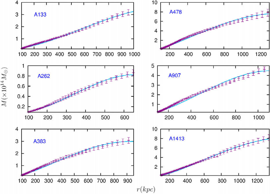
Fig. 1 Dynamical mass vs. radius for the galaxy clusters. Dynamical mass vs. radius for the first 6 clusters of galaxies, with the best-fit parameters as summarized in Table 1. The points with uncertainty bars are the 1σ dynamical masses obtained in Vikhlinin et al. (2006). The solid line is the best fit obtained with our model. The color figure can be viewed online.
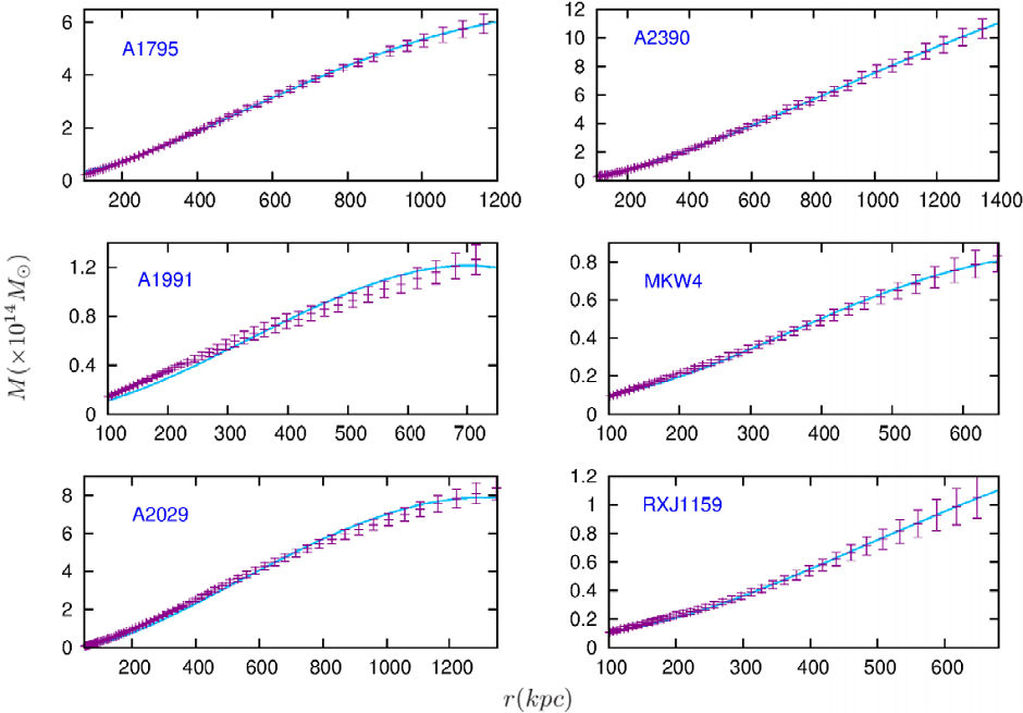
Fig. 2 Dynamical mass vs. radius for the galaxy clusters. The same as Figure 1 for the remaining 6 clusters of galaxies. The color figure can be viewed online.
From the best-fit analysis, we see that our model is capable to account for the total dynamical masses of the 12 clusters of galaxies, except at the very inner regions for some of them, a persistent behavior more accentuated for A907 and A1991. Notice that the parameter A quantifies the extra Newtonian-like contribution to the dynamical mass [cf. equation (67)], and the parameters B and r s are present in the Φ(2) c term only [equation (66)]. As can be seen in Table 2, there are two systems, A1413 and A2029, for which the estimated parameter r s is very far from the mean value for the other clusters. Comparing its contribution to the acceleration with respect to the other two terms in equation (67), we found that the dominant second order term is the one with the parameter A, and the contribution of the derivative of the integral (66) is very small (since r s appears inside a logarithm and because of the particular combination of the functions in such equation).
From the figures, we see that the “MOND-like” relativistic correction of our model is better in the outer regions of the galaxy clusters than standard MOND, which needs extra matter to fit the observations in these systems. Also, the second order perturbation analysis of the metric theory f(χ) = χ
3/2
is capable to account for the observations of the rotation curves of spiral galaxies and the Tully-Fisher relation, and the gravitational lensing in individual, groups and clusters of galaxies (Mendoza et al. 2013). In this work, we keep fixed those parameters at
Up to now it has generally been thought that a MOND-like extended theory of gravity was not able to explain the dynamics of clusters of galaxies without the necessary introduction of some sort of unknown DM component. Our aim has been to show that in order to account for this dynamical description without the inclusion of DM, it is necessary to introduce relativistic corrections in the proposed extended theory. To do so, we have chosen the particular f(χ) = χ 3/2 MOND-like metric extension (Bernal et al. 2011b), which has also proved to be in good agreement with gravitational lensing of individual, groups and clusters of galaxies, and with the dynamics of the Universe, providing an accelerated expansion without the introduction of any dark matter and/or energy entities (see Mendoza 2015, for a review).
A similar analogy occurred when studying the orbit of Mercury about a century ago. Its motions were mostly understood with Newton’s theory of gravity. However it was necessary to add relativistic corrections to the underlying gravitational theory to account for the precession of its orbit. Mercury orbits at a velocity v ≈ 50km/s, implying v/c ≈ 10−4 and already relativistic corrections are required. Typical velocities of clusters of galaxies are v ≈ 103 km/s, with v/c ≈ 10−3. This means that the dynamics of clusters of galaxies are about one order of magnitude more relativistic than the orbital velocity of Mercury and so, if the latter required relativistic corrections, then the corrections needed to describe the dynamics of clusters of galaxies are even more important.

