


 nova página do texto(beta)
 Inglês (pdf)
 Artigo em XML
 Referências do artigo
 Enviar este artigo por email
 Citado por SciELO
  Similares em
SciELO
Similares em
SciELO 
 Permalink
1. INTRODUCTION
This high amplitude Delta Scuti (HADS) star, V2455 Cyg, was first described recently by Wils et al. (2003), who found it to be a new variable star. They reported that its variability was suspected by Yoss et al. (1991) who derived the following characteristics: a distance of 215 pc, an absolute magnitude of 2.2 and a total space velocity S of 32 km/s. They also determined V = 8.86, and (B-V)=+0.27 which classifies this star as spectral type F2. A period of 0.094206 d was proposed by Piquard (2001) from available Tycho data.
2. OBSERVATIONS
This article is a product of a long campaign de-voted to several objects, one of which was NGC 6633 (Peña et al. 2017, Paper I) already published. An-other article in progress is devoted to the open clusters IC 4665, NGC 6871 and Dzim 5 (Paper II). In these works we have explained in detail the procedures followed in the acquisition and reduction of the data. Here we present the data of the pulsating variable V2455, a HADS star. The observations were done at the Observatorio Astrónomico Nacional of San Pedro Mártir (SPM) in México. Table 1 presents the log of observations, as well as the new times of maximum light.
TABLE 1 LOG OF OBSERVING SEASONS OF V 2455 CYG
| Date year/month/day | Observer | Number of points | Observed time (day) | Nmax | HJD (day) |
|---|---|---|---|---|---|
| 2016/06/26 | ARL | 85 | 0.08 | 1 | 2457565 |
| 2016/06/27 | ARL | 32 | 0.06 | 0 | 2457566 |
| 2016/06/28 | ARL | 62 | 0.07 | 0 | 2457567 |
| 2016/07/05 | CVR | 41 | 0.09 | 1 | 2457574 |
| 2016/07/06 | CVR | 48 | 0.11 | 1 | 2457575 |
2.1. Data Acquisition and Reduction
The observations were done in the summer of 2016, along with those of other variable stars and clusters. The procedure to determine the physical parameters has been reported elsewhere (Peña et al., 2016). The photometric system, if well-defined and calibrated, provides an efficient method to investigate physical conditions, such as effective temperature and surface gravity, using a direct comparison of the unreddened indexes with those obtained from theoretical models. These calibrations have been described and used in previous analyses (Peña & Peniche; 1994; Peña & Sareyan, 2006).
The observations consisted of one long season with two different observers (ARL and CVR), one in June (22 to 30 by ARL) and the other in July, 2016 (1 to 8 by CVR) with different target objects in each one, although two were obtained in both sea-sons (NGC 6633 (Paper I) and V2455 Cyg).
The reduction was done considering both seasons together to make a longer season in order to increase the accuracy provided by the standard stars. Over the five nights of observation of V 2455 Cyg, the following procedure was used: for each measurement we took at least five ten-second integrations of each star and one ten-second integration of the sky for the uvby filters and the narrow and wide filters that define Hβ.
We also observed a series of standard stars nightly to transform the data into the standard system. The chosen system was that defined by the reported values of Olsen (1983) although some standard bright stars were chosen from the Astronomical Almanac (2006). The transformation equations are those defined by Crawford & Barnes (1970) and by Crawford & Mander (1966).
The coefficients defined by the following equations and which adjusted the data to the standard system were:
In these equations the coefficients D, F, H and are the slope coefficients for (b − y), m 1, c 1 and β, respectively. The coefficients B, J and I are the color terms of V, m 1, and c 1. The averaged transformation coefficients of the season are listed in Table 2 along with their standard deviations. Season errors were evaluated with the eighteen standard stars observed for a total of 272 observed points. These un-certainties were calculated through the differences in magnitude and colors for all nights, for (V , b − y, m 1, c 1 and β) as (0.024, 0.010, 0.011, 0.015, 0.015) respectively, which provide a numerical evaluation of our uncertainties for the season. Emphasis is made on the large range of standard stars in the magnitude and color ranges: V: (5.0, 8.8); (b − y):(-0.06, 0.80); m 1:(0.10, 0.68); c 1:(0.11, 1.18) and β:(2.60, 2.82).
TABLE 2 TRANSFORMATION COEFFICIENTS OBTAINED FOR THE OBSERVING SEASON
| Season | B | D | F | J | H | I | L |
|---|---|---|---|---|---|---|---|
| Summer 2016 | 0.006 | 0.971 | 1.049 | 0.033 | 1.016 | 0.103 | −1.356 |
| σ | 0.033 | 0.005 | 0.051 | 0.016 | 0.034 | 0.052 | 0.044 |
Table 3 lists a sample of the photometric values of the observed star. The complete data set will be published elsewhere. In this table Columns 1 to 4 list the Strömgren values V, (b − y), m1 and c1, respectively; Column 5, Hβ, whereas Column 6 reports the time of the observation in HJD. The photometry is presented in Figure 1.
TABLE 3 uvby − β PHOTOELECTRIC PHOTOMETRY OF V2455 CYG
| V | (b − y) | m 1 | c 1 | β | HJD |
|---|---|---|---|---|---|
| 9.011 | 0.195 | 0.169 | 0.759 | 2457565.8898 | |
| 9.022 | 0.195 | 0.167 | 0.761 | 2.732 | 2457565.8902 |
| 9.007 | 0.200 | 0.167 | 0.763 | 2457565.8913 | |
| 9.010 | 0.206 | 0.161 | 0.768 | 2457565.8937 | |
| 9.009 | 0.210 | 0.154 | 0.775 | 2.749 | 2457565.8941 |

3. PERIOD DETERMINATION
To determine the period behavior of V 2455 Cyg the following methods were employed: (1) differences of consecutive times of maximum light were evaluated to determine a coarse period; (2) a time series analysis of the data set was utilized; (3) O − C differences were calculated using a compiled collection of times of maximum light (MSDR); (4) Period de-termination through O − C differences minimization (PDDM).
The previously determined ephemerides equations as well as the newly determined ones are listed in Table 4. In this table Column 1 indicates the method followed; Columns 2 and 3 the elements of the proposed ephemerides. The goodness of the elements can be discriminated by the mean and standard deviation values listed in Columns 4 and 5.
TABLE 4 V 2455 CYG EPHEMERIDES EQUATIONS
| Method | T 0 | P | Mean | Std Dev |
|---|---|---|---|---|
| Wils et al. (2003) | 2452885.3992 ± 0.0001 | 0.0942075 ± 3 × 10⁻⁷ | −0.0031 | 0.0213 |
| DCTM (consecutive Tmax) | 0.0944 | −0.0041 | 0.0189 | |
| Period04 (uvby − β data) | 0.0942080868 | −0.0136 | 0.0195 | |
| MSDR (O − C) | 2452885.3996 ± 0.0002 | 0.094205989 ± 1.2 × 10⁻⁸ | 0.0009 | 0.0066 |
| PDDM (Chord lenght) | 2457575.9157 | 0.094205855 | ||
| PDDM (Sinusoidal fit) | 2457575.9157 | 0.094205903 |
3.1. Differences of Consecutive Times of Maximum Light, DCTM
To determine the period from scratch, as a first guess we considered the period calculated through the differences of two or three times of maxima that were observed on the same night. Since they are separated by only one cycle they are, by definition, one period apart. The sample of periods determined in this fashion is constituted of 44 times of maxima difference and was compiled from both those listed in the literature and the few that we measured two years later (Table 5). There were fourteen consecutive times of maxima; the mean value was 0.0944 ± 0.0006 (d). The uncertainty is merely the standard deviation of the mean.
TABLE 5 COMPILED TIMES OF MAXIMA OF THE HADS STAR V 2455 CYG
| Time of Maximum | Reference |
|---|---|
| 2452885.3991 | Wils03 |
| 2452885.3993 | Wils03 |
| 2452887.3777 | Wils03 |
| 245287.3778 | Wils03 |
| 2452887.4720 | Wils03 |
| 2452887.4720 | Wils03 |
| 2452887.5656 | Wils03 |
| 2452887.5658 | Wils03 |
| 2452887.6599 | Wils03 |
| 2452928.2634 | Wils03 |
| 2452928.3582 | Wils03 |
| 2452928.4520 | Wils03 |
| 2452928.5465 | Wils03 |
| 2452929.2996 | Wils03 |
| 2452929.3940 | Wils03 |
| 2452929.4885 | Wils03 |
| 2452929.5823 | Wils03 |
| 2452931.4667 | Wils03 |
| 2454357.5561 | wils09 |
| 2454642.4354 | wils09 |
| 2454642.5296 | wils09 |
| 2454646.4860 | wils09 |
| 2454652.5157 | wils09 |
| 2454694.4383 | wils09 |
| 2454694.5327 | wils09 |
| 2454730.3298 | wils09 |
| 2454730.4239 | wils09 |
| 2454730.5182 | wils09 |
| 2454730.6126 | wils09 |
| 2454758.4973 | wils09 |
| 2454759.3447 | wils09 |
| 2454759.4389 | wils09 |
| 2454759.5332 | wils09 |
| 2456862.3963 | Hubsecher15 |
| 2456862.4903 | Hubsecher15 |
| 2456862.5842 | Hubsecher15 |
| 2456867.4869 | Hubsecher15b |
| 2456867.5832 | Hubsecher15b |
| 2456914.5926 | Hubsecher15b |
| 2456914.5930 | Hubsecher15b |
| 2457565.9307 | pp |
| 2457574.8801 | pp |
| 2457575.9157 | pp |
This period served as seed and was utilized with T 0, the first time of maximum of Wils et al. (2003), and the epochs in the list of times of maximum light, Table 5, to calculate new ephemerides through a linear regression of epoch vs. HJD, thus determining refined values of T 0 and P . The period we established in this fashion (0.0944 d) is in agreement with the assumed period reported in the literature. The results of this method are presented in the second row of Table 4.
3.2. Time Series
As a second method to determine the period we used a time series method favored by the δ Scuti star community: Period04 (Lenz & Breger, 2005). The V magnitude of the uvby − β set was analyzed with this code.
The analysis of these data gave the results listed in Table 6 with a zero point of 8.8184 mag, residuals of 0.0178 mag and 5 iterations. The analysis of Period04 is presented in Figure 2. Beginning at the top is the power spectra of the original data; followed by the consecutive set of residuals. The scale of the axis is the same to show the relative importance of the residuals. The frequencies obtained from this analysis are presented in Table 6. Three different frequency values are reported, but one must realize that F 2 = 2 F 1 and F 3 = 3 F 1, that the second and third frequencies are multiples of the first.

Fig. 2 Power spectra of V 2455 Cyg with the SPM data. Top to bottom: first is the power spectra of the original data; then, the sets of residuals. The scale of the Y axis is the same to show the relative importance of each frequency.
3.3. O − C differences
Before calculating the coefficients of the ephemeris equation, we searched the literature for previous papers related to V 2455 Cyg. Only one source conducted studies of the O − C behavior of this particular object (Wils et al., 2003). The reported ephemerides are listed in Table 4; the newly observed ephemerides are also presented.
3.4. Period Determination Through Minimization of the Standard Deviation of the O − C Residuals (MSDR)
The well-known O − C diagram method is a tool utilized to compare and analyze the difference between the observations and the calculated value obtained with the model; in this case, the ephemerides equation. A good reference for this method can be found in Sterken (2005).
To find the ephemerides equation of the variability of V2455 Cyg we implemented a method based on the minimization of the standard deviation of multiple O − C diagrams for V2455 Cyg (see Peña et al., 2016 for details). This method is based on the minimization of the standard deviation of the O−C residuals by considering that the model must be fairly close to the data. Therefore, its differences tend to zero and the standard deviation has to be close to zero. The first step was to calculate the mean of the differences of all the consecutive times of maxima available in the literature (first method) and its standard deviation. All these differences of consecutive times of maxima have the approximate length of the period of the star. Then, with each of the periods given in the range provided by the mean of the consecutive, plus and minus its standard deviation, the number of cycles E was calculated for these multiple O − C diagrams. In all cases, the T 0 utilized was the oldest time of maxima in the literature. The step precision in this range was of 1 × 10⁻⁹. After obtaining the number of cycles for each period, a linear fit was performed to every set of times of maximum with the cycle number E (HJD vs. E). With the new fitted parameters, the diagrams were calculated as well as their standard deviation. Finally, the diagram with the smallest standard deviation of the residuals was selected and the parameters with which it was calculated are taken to be the parameters of the ephemerides equation.
Sweeping around the average of the differences of consecutive times of maxima within a short period range, taking as limits the standard deviation of the differences around 0.0943052 d, and utilizing the minimization of the standard deviation of the O − C values as criterion of goodness, the best period is 0.094205989 d (Figure 3). The resulting ephemerides equation is
Even with the maximum resolution (1 × 10⁻⁹) in the MSDR method, there was some scatter around the minimum in the Standard Deviation vs. Period plot (Figure 3). To clarify this, a binning procedure was implemented. For this binning the size of the intervals was 1 × 10⁻⁸. After this operation the minimum value of the standard deviation was checked. This was 0.094205989, which is the same as the original before the binning procedure. Continuing with the analysis, two new binning procedures were implemented, but this time with intervals of 1 × 10⁻⁷ and 1 × 10⁻⁶. In the first new case, the period for the minimum standard deviation remained the same, but in the final case the period with the minimum standard deviation was 0.094206015. The value of the period changes only after the size of the intervals for the binning is three orders of magnitude larger than the original precision.

Fig. 3 Standard deviation vs. period. This diagram served to determine the best period. In the upper panel the original data that served to determine the best period are shown. In the lower panel the data have been binned with a window of 1 × 10⁻⁶.
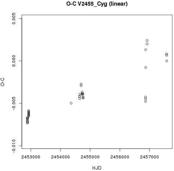
With these elements we calculated the O − C residuals which are shown schematically in Figure 4. They are clearly fitted by straight line, which implies a constant period (at least at this stage) with a time basis of 12.8 yrs.

3.5. Period Determination Through an O − C Differences Minimization (PDDM)
We implemented a method based on the idea of searching for the period which minimizes the chord length which links all the points in the O−C diagram for different values of the periods. Being a classical O−C diagram, we plotted the time in the x-axis and the O − C values in the y-axis. Since in the x-axis distances remain constant, we just concentrated on the change in the distance in the y-axis generated by each period. Once the difference was calculated for each period, the minimum one indicated, at this stage, the best period (period determination through an O − C differences minimization PDDM).
We considered the set of TMAX listed in Table 5. Given the mean period determined from the consecutive times of maxima and the associated standard deviation, (0.0938 days and 0.0944 days), we calcuated values of epoch and O − C by sweeping the period in the range provided by the standard deviation limits, calculating 595,956 steps, a number fixed by the the difference of the deviation limits and the desired precision of one billionth. This provided the new period for the minimum difference (Figure 5). The T0 time used for the present analysis was the one of the last observation run, 2457575.9157, be-cause we are certain of its precision. As a result we determined the linear ephemerides equation as:

Figure 6 shows the O − C diagram for the ephemerides equation found by the above method (PDDM).
Assuming the wave behavior is caused by a light travel time effect (LTT) as a part of the mechanics of the system, we adjusted a sinusoidal function to the O − C, performing a fit with the Levenberg-Marquardt algorithm for the best 1,000 O − C lengths. This would be, in this particular case, an-other way of finding the best period (if the LTT effect is present) and, at the same time, the sinusoidal function that gave us a first approach to the orbital period of a two body system. The parameters which best represent the system are listed in Table 7. The parameter used to test the goodness of the fit is the residual sum of squares RSS. Then, we plotted the periods of the best O − C lengths vs the RSS value of every fit (Figure 7).
TABLE 7 EQUATION PARAMETERS FOR THE SINUSOIDAL FIT OF THE LINEAR O − C
| Value | PDDM |
|---|---|
| Z | −13.62 × 10⁻⁴ |
| Ω | 3.14 × 10⁻⁴ |
| A | −27.93 × 10⁻⁴ |
| Φ | −27.14 |
| RSS | 6.1 × 10⁻⁵ |

After this, the ephemeris equation was set as:
As can be seen, we do not have enough data to say more about the O − C diagram. The parameters presented in Table 7 are shown schematically in Figure 8.

3.6. Period Determination Conclusions
V 2455 Cyg has been little observed. Since the first report more information has been gathered, but no period analysis has been done. In the present paper, different approaches were utilized to determine the stability of the pulsation. First, differences of consecutive times of maximum light were evaluated to determine a coarse period. The second method utilized time series analyses. The set employed was that of the V magnitude of the uvby −β photometry of the present paper. However, we had a very limited time coverage, only 10 d, merely 107 cycles. The third and fourth methods utilized the entire coverage of this star since its discovery, with the times of maxi-mum light, which in this case are 4691 d or 12.8 years (49795 cycles). The four methods used the available data up to now. The goodness of each method and that proposed previously were determined using the mean and the standard deviation of the residuals of the O − C values, the minimum chord length, and RSS (residual sum of squares) for the sinusoidal fit-ting of the O − C diagrams. They were obtained for each ephemeris listed in Table 4 and numerically they are listed in Columns 4, 5 and 6 of this table. It is quite evident that the MSDR method yields the smallest standard deviations for the O − C residuals, but if we consider the sinusoidal behavior as part of the mechanics of the system, the PDDM gives us the best ephemerides equation.
However, this star was discovered to be a variable very recently and has been observed too little to be able to make a solid conclusion since a large spread can be seen in a section of the O − C diagram (Figures 4 and 6). Those points belong to the observational group of Hubscher (2015, 2015b). There are two possible explanations for the large spreads: an inaccurate determination of the times of maxima for those seasons or the possibility that this group is a set of observations acquired during one of the changes in the period inflicted by the presence of a second body which corresponds to the LTT effect mentioned in the PDDM method. We feel that more time must pass, with a more frequent sampling, before we can definitively arrive at conclusions about the pulsational nature of V 2455 Cyg, the LTT effect, and a possible secular variation.
TABLE 8 REDDENING AND UNREDDENED PARAMETERS OF V 2455 CYG
| Phase | E(b − y) | (b − y) 0 | m 0 | c 0 | Hβ | M V |
|---|---|---|---|---|---|---|
| 0.05 | 0.006 | 0.157 | 0.177 | 0.851 | 2.778 | 1.737 |
| 0.15 | 0.002 | 0.122 | 0.179 | 0.953 | 2.809 | 1.313 |
| 0.25 | 0.001 | 0.127 | 0.175 | 0.968 | 2.801 | 1.075 |
| 0.35 | 0.005 | 0.145 | 0.171 | 0.920 | 2.784 | 1.251 |
| 0.45 | 0.007 | 0.159 | 0.169 | 0.871 | 2.772 | 1.511 |
| 0.55 | 0.002 | 0.180 | 0.166 | 0.833 | 2.751 | 1.548 |
| 0.65 | 0.002 | 0.197 | 0.167 | 0.788 | 2.734 | 1.634 |
| 0.75 | 0.005 | 0.201 | 0.165 | 0.768 | 2.732 | 1.758 |
| 0.85 | 0.006 | 0.199 | 0.163 | 0.763 | 2.735 | 1.859 |
| 0.95 | 0.004 | 0.184 | 0.170 | 0.776 | 2.752 | 2.066 |
4. PHYSICAL PARAMETERS
The physical parameters can be determined utilizing the uvby − β photoelectric photometry and the adequate empirical calibrations. These calibrations were proposed by Nissen (1988) for A and F type stars. Therefore, it is necessary to first deter-mine if this star varies in this range of spectral class. It was reported by Yoss et al. (1991) that V2455 Cyg is spectral type F2, but it has a reported MK spectral type A9. The spectral type can be determined very accurately with the uvby − β photometric data. We determined its unreddened photometric indexes [m1] and [c1] and positioned it in the plot determined for Alpha Per (Paper I), whose stars have well-determined spectral types. This is presented in Figure 9, where we can see that the spectral type is earlier, since it ranges between A2 and F0.

Application of the numerical unreddening package (see Peña & Martinez, 2014 for a detailed de-scription) gives the results listed in Table 7 for V 2455 Cyg.
Since there were so many uvby − β photoelectric data points, we calculated the mean values in phase bins of 0.05 step. These mean values are listed in Table 7. This table lists (ordered by increasing phase) in the first column, the phase; subsequent columns present the reddening, the unreddened indexes, and the absolute magnitude. Mean values were calculated for E(b − y) for two cases: (i) the whole data sample and (ii) in phase limits between 0.3 and 0.8, which is customary for pulsating stars to avoid the maximum. It gave, for the whole cycle, values of 0.004 ± 0.007; 7.2 ± 0.4 and 284 ± 47 for E(b − y), DM and distance (in pc), respectively whereas for the mentioned phase limits, we obtained, 0.004 ± 0.007; 7.3 ± 0.3 and 292 ± 37 respectively. For the metal content [Fe/H] it gives 0.04 ± 0.11 and 0.01 ± 0.11, respectively. The uncertainty is merely the standard deviation. In the case of the reddening, most of the values of the spectral type in the F stage of V 2455 Cyg produced negative values which are non-physical. In those cases we forced the reddening to be zero. If the negative values are included, the mean E(b − y) is 0.009 ± 0.038.
To determine the range of effective temperature and surface gravity over which V2455 Cyg varies we must locate the unreddened points on some theoretical grids, such as those of LGK86 calculated from uvby − β photometric data for several metallicities. Hence, in order to locate our unreddened points on the theoretical grids, a metallicity has to be assumed. The metallicity of V 2455 Cyg can be determined from the uvby − β photometry when the star passes through the F type stage (Nissen, 1988). We determined a mean metallicity of [Fe/H]= 0.042 ± 0.106 for the whole data sample, and of 0.011 ± 0.113 for the values within the specified 0.3 to 0.8 phase limits. The model which is applicable is, therefore, that of solar composition [Fe/H]= 0.0.
To decrease the noise and to see the variation of the star in phase, mean values of the unreddened colors were calculated in phase bins of 0.1 starting at phase 0.05. As can be seen in Figure 10, the case of [Fe/H] = 0.0 the star varies between effective temperature 7200 K and 7900 K; the sur-face gravity log g varies between 3.6 and 3.9. Table 9 lists these values. Column 1 shows the phase, Column 2 lists the temperature obtained from the plot for each [Fe/H] value; Column 3, the effective temperature obtained from the theoretical relation reported by Rodriguez (1989) based on a relation of Petersen & Jorgensen (1972, hereinafter P&J72) TE = 6850 + 1250 × (β − 2.684)/0.144 for each value, averaged in the corresponding phase bin, and Column 4, the mean value. Column 5 shows the surface gravity log g taken from the plot.

TABLE 9 EFFECTIVE TEMPERATURE AND SURFACE GRAVITY OF V 2455 CYG AS A FUNCTION OF PHASE
| phase | T e(0.0) | T e(P&J72) | T e(Mean) | log g(0.0) |
|---|---|---|---|---|
| 0.05 | 7600 | 7663 | 7232 | 3.9 |
| 0.15 | 7900 | 7931 | 7916 | 3.8 |
| 0.25 | 7800 | 7864 | 7832 | 3.5 |
| 0.35 | 7700 | 7717 | 7708 | 3.5 |
| 0.45 | 7600 | 7615 | 7607 | 3.5 |
| 0.55 | 7300 | 7431 | 7366 | 3.5 |
| 0.65 | 7200 | 7282 | 7241 | 3.5 |
| 0.75 | 7200 | 7266 | 7233 | 3.5 |
| 0.85 | 7300 | 7291 | 7296 | 3.5 |
Note: Values in parenthesis specify the [Fe/H] values.
4.1. Physical Parameters: Conclusions
New uvby −β photoelectric photometry observations were carried out for the HADS star V 2455 Cyg. From these observations we first determined its spectral type, which varies between A3V and F0V, different from that previously found. From Nissen’s (1988) calibrations the reddening was determined, as well as the unreddened indexes. This served to obtain the physical characteristics of the star: effective temperature in a range from 7200 K to 7900 K and log g from 3.6 to 3.9 with two methods: (1) from the location of the unreddened indexes in the LGK86 grids and (2) through the theoretical relation (P&J72).
5. CONCLUSIONS
We studied V2455 Cyg, which was recently de-scribed by Wils et al.(2003). In the present study we demonstrated that V 2455 Cyg is pulsating with one stable period. We carried out three different procedures in the analysis of the periodic content of the star: difference calculation of consecutive times of maximum, the canonical Fourier transform using Period04, and using the compilation of all the times of maximum light since its discovery by minimization of the standard deviation of the O−C Residuals (MSDR). All converge to the ephemerides equation of
By means of uvby − β photoelectric photometry we were able to determine its spectral type. We have classified this star spectroscopically between types A2 and F0. With the uvby − β data and the empirical calibrations of Nissen (1988) we were able to determine the reddening of each point. With this in-formation we obtained the unreddened color indexes. Evaluating between phases in the range 0.3 to 0.8 we obtained: 0.004 ± 0.007; 7.3 ± 0.3 and 292 ± 37 for E(b − y), DM and distance (in pc), respectively. The unreddened color indexes were compared with the output uvby − β grids of the models of LGK86. With this we were able to determine an effective temperature between 7200 K and 7900 K and a surface gravity log g from 3.6 to 3.9. To do this we had to assume a metal content [Fe/H] from the measurements when the star passes through the F spectral type stage. We determined a mean metallicity of [Fe/H]= 0.042±0.106 for the whole data sample, and of 0.011±0.113 for the values within the specified 0.3 to 0.8 phase limits. The model which is applicable is, therefore, that of solar composition [Fe/H]= 0.0.

