1. Introduction

The nature of a low-mass eclipsing binary KIC 12004834 with 14^m.7180 in Kepler band is studied here. KIC 12004834, whose nature is different from the classical UV Ceti type stars of spectral type dMe due to its being a binary system, was observed by ^{Watson (2006)} for the first time. Magnitudes of the system were given as J = 12^m.007, H = 11^m.407, K = 11^m.170 by ^{Cutri et al. (2003)}. Although there are no further studies in the literature, some estimated parameters of the system were given by ^{Coughlin et al. (2011)}, using calibrations to derive the parameters. Taking T_eff = 3576 K, the orbital inclination (i) was found to be 72◦.47, while the masses were found to be M₁ = 0.48 M⊙ and M₂ = 0.34 M⊙. In addition, the radii were computed as R₁ = 0.48 R⊙ and R₂ = 0.35 R⊙. Like ^{Coughlin et al. (2011)}, taking T_eff = 3576 K, ^{Slawson et al. (2011)} found log(g) as 4.217 cm/s². There are several approaches to obtain the temperatures of its components. Coughlin et al. (2011) gave the temperatures as T₁ =3620 K for the primary and T ₂ =3468 K for the secondary. ^{Armstrong et al. (2014)} gave T ₁ =3511 K for the primary and T ₂ =3512 K for the secondary.

KIC 12004834 was mentioned as a chromospherically active system for the first time by ^{Debosscher et al. (2011)}. In addition, a dominant flare activity was also reported by ^{Balona (2015)}. Considering the estimated parameters of the system; KIC 12004834 is a low-mass close binary with a chromospherically active component. This makes the system an important object in the astrophysical sense. This is because the system exhibits not only spots, but also flare activity. A flaring star being a component of an eclipsing binary system is a rare phenomenon among the UV Ceti type stars. However, the red dwarf abundance is about 65% in our Galaxy, and seventy-five percent of them exhibit flare activity (^{Rodonó 1986}). Thus, almost half of the stars in our galaxy should exhibit flare activity. The number of eclipsing binaries with a flaring component is nowadays increasing, thanks to space missions such the Kepler and Corot satellites.

Because of its effects on stellar evolution, flare activity is very important in astrophysics in terms of its sources and mechanism. Although the first flare was observed on the solar surface by R. C. Carrington and R. Hodgson on September 1, 1859 (^{Carrington 1859}; ^{Hodgson 1859}), there are still unsolved problems, for instance, the different mass loss rate seen among stars of different spectral types, the different flare energy levels detected for stars of different spectral types (^{Gershberg & Shakhovskaya 1983}; ^{Haisch et al. 1991}; ^{Gershberg 2005}; ^{Benz 2008}).

At this point, photometric data accumulated from the eclipsing binaries with a chromospherically active component can give some clues for these problems. Recently, several eclipsing binary stars, where one of the components is chromospherically active have been discovered by the Kepler Mission (^{Borucki et al. 2010}; ^{Koch et al. 2010}; ^{Caldwell et al. 2010}). Most of them have an interesting nature. These chromospherically active components exhibit flare events and also rapidly evolving stellar spots (^{Balona 2015}). Although the light variations due to the cool spots have remarkably small amplitudes, their shapes change over short time intervals, from one cycle to the next one (^{Yoldaş & Dal 2016}, ²⁰¹⁷; Özdarcan et al. 2017).

In this study, the variations of the times of minima are analysed (see § 2.1). The light curve of KIC 12004834 is studied (§ 2.2) for the first time in the literature in order to find the physical properties of the components. Then, the flares occurring on the chromospherically active component are used to model the nature of the magnetic activity of the system as described in § 2.3. The results obtained are given in § 3, comparing the active component with its analogue discovered in the Kepler Mission.

2. Data and analyses

The data analysed in this study are the detrended short cadence data from the Kepler Mission Database (^{Borucki et al. 2010}; ^{Koch et al. 2010}; ^{Caldwell et al. 2010}; ^{Slawson et al. 2011}; ^{Matijevič et al. 2012}). In the analyses, the data of quarters Q10.1, Q10.2 and Q10.3 are used (^{Murphy 2012}; ^{Murphy et al. 2013}), whose quality and sensitivity are the highest ones ever reached (^{Jenkins et al. 2010a},^b).

After removing all the observations with large errors from the data, and using the ephemeris taken from the Kepler Mission database, the phases are computed for all data, and the obtained light curves are shown in Figure 1. Because of the study’s format, the detrended short cadence data were used in the analysis instead of those of the long cadence. The data were arranged in suitable formats for different analyses, such as the light curve analysis and the flare event calculations.

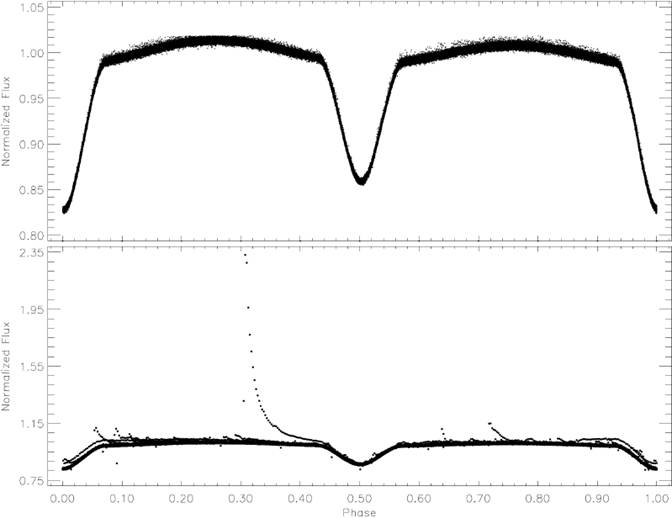
Fig. 1 Whole light curve of KIC 12004834 obtained from the data taken from the Kepler Mission database. In the bottom panel, the light curve is plotted along the orbital cycle with the flare activity, while it is plotted without the flare activity in the upper panel. 

2.1. Orbital Period Variation

The times of minima in the light curves were computed from short cadence data without any corrections. We used just short cadence data, because the system has a very short orbital period. The whole shape of the minima is not seen in the long cadence data. The minima times were computed with a script according to the method described by ^{Kwee & van Woerden (1956)}. The (O − C) _I residuals were determined for each minimum time. Examining the times of minima indicated that some of them have very large errors. These errors are sometimes caused by scattered observations; while some of them are caused by the flare activity occurring during these minima. All the minima times with large errors were removed from the (O −C) data. Finally, 688 minima times were determined in the analyses.

Using the epoch of 2455002.041 and the orbital period of 0.2623168 day given in the Kepler Eclipsing Binary Catalogue¹ by ^{Slawson et al. (2011)}, we computed the (O − C) _I residuals. Then, using the Least-Squares method, we applied a linear correction to these residuals. The linear correction revealed that the (O − C) _I residuals had a linear trend with a small slope; the distribution of the (O − C) _I residuals seems to be linear, needing just a zero point correction. After the linear correction, we obtained the new ephemerides given in equation (1) and the (O − C) _II residuals:

JD(Bary.)=24 55002.04164(14)+0d.262317(1) × E. (1)

The (O − C) _I and (O − C) _II residuals are listed in Table 1. In the table, the minima times, cycles, the minima type, (O − C)_I and (O − C) _II residuals are listed, respectively. An interesting variation is seen in the (O − C) _II residuals plotted versus time in Figure 2.

Fig. 2 The variations of time of minimum residuals of (O − C) _I and (O − C) _II obtained by applying a linear correction. In the bottom panel, the filled blue circles represent the primary minima; the filled red circles represent the secondary minima. In the upper panel all the residuals are plotted with filled black circles, while the red line represents a linear fit. The color figure can be viewed online. 

According to the studies of ^{Tran et al. (2013)} on contact binaries, if one of the components of an eclipsing binary system exhibits stellar spot activity on its surface, there must be a separation between the (O−C) _II residuals of the primary and secondary minima. ^{Debosscher et al. (2011)} and ^{Balona (2015)} mentioned that the system exhibits chromospheric activity. In the case of KIC 12004834 considered as a very close binary, we firstly examined whether there was any separation in the primary and secondary minimum (O − C) _II residuals. As shown in the upper panel of Figure 2, there is an evident separation between the primary and secondary minima residuals. Secondly, the analysis indicates that the best fit is derived by a linear function for the distribution of (O − C) _I . The obtained fit is shown in the lower panel of is Figure 2.

2.2. Light Curve Analysis

The light curve of KIC 12004834 was analyzed by the PHOEBE V.0.32 software (^{Prša & Zwitter 2005}) which depends on the 2003 version of the Wilson-Devinney Code (^{Wilson & Devinney 1971}; ^{Wilson 1990}) to compute the physical parameters of each component. In the analyses, the averaged data were computed phase by phase with an interval of 0.001 to decrease the scattering. Although several modes were tried in the light curve analyses, astrophysically acceptable parameters were obtained only for the detached system mode.

The PHOEBE V.0.32, needs a temperature value for the primary component. We determined its temperature from the J HK brightness given by ^{Cutri et al. (2003)}. The de-reddened colors were found to be (H − K)_o = 0^m.252 and (J − K)_o = 0^m.629. Then a temperature value of 4220±20 K corresponding to the de-reddened colours was obtained by using the calibrations given by ^{Tokunaga (2000)}. We accepted this value as the primary component temperature. The temperature of the secondary component was taken as an adjustable free parameter. In the analyses, some coefficients, such as the albedos (A ₁ and A ₂), the gravity-darkening coefficients (g ₁ and g ₂) and the limb-darkening coefficients (x ₁ and x ₂), were taken from the tables given by ^{Lucy (1967)}; ^{Rucinski (1969)}; ^{Van Hamme (1993)}, considering the possible temperatures of both components. The rest of the parameters, such as the dimensionless potentials (Ω₁ and Ω₂), the fractional luminosity (L ₁) of the primary component, the inclination (i) and the mass ratio (q) of the system, were taken as adjustable free parameters.

The computed values of the free parameters are tabulated in Table 2, while the synthetic light curve derived by these parameters is shown in Figure 3. As the table shows, some errors are smaller than the expected values. However, the errors given in the table were computed by the PHOEBE V.0.32, depending on ^{Taylor (1997)}. In fact the χ² was computed as 3.15×10^-3 from the Kepler short cadence data. The 3D model of Roche geometry obtained with these parameters is shown in Figure 4.

Table 2 Parameters obtained from the light curve analysis of KIC 12004834 

Parameter	Value
q	0.743 ± 0.001
i (º)	75.89 ± 0.03
T1 (K)	4220 (fixed)
T2 (K)	4001 ± 11
Ω1	4.308 ± 0.004
Ω2	5.485 ± 0.007
L1/L2	0.245 ± 0.067
g1, g2	0.32 (fixed)
A1, A2	0.32 (fixed)
x1,bol , x2,bol	0.377, 0.001 (fixed)
x1, x2	0.369, 0.001 (fixed)
< r1 >	0.287 ± 0.001
< r2 >	0.172 ± 0.001
Co-LatSpot(rad)	1.920 ± 0.004
LongSpot(rad)	1.710 ± 0.002
RSpot(rad)	0.244 ± 0.003
T f Spot	0.960 ± 0.001

Fig. 3 The light curve along the orbital cycle, from BJD 2455739.94 to 2455829.13. In the figure, the filled circles represent the observations, while the red smooth line represents the synthetic light curve. The color figure can be viewed online. 

Fig. 4 The 3D model of Roche geometry and spotted area distribution derived from the light curve analysis is shown for different phases, such as (a) 0.00, (b) 0.25, (c) 0.50, (d) 0.75. The color figure can be viewed online. 

It should be noted that we obtained a solution after some iterations in the detached system mode of the Wilson-Devinney Code (^{Wilson & Devinney 1971}; ^{Wilson 1990}). Although the synthetic curve fitted the observations very well, it was revealed that it did not fit the observations around phase 0.27. To solve this mismatched part of synthetic light curve, we assumed that there is a spotted area on a component, considering the flare activity. We assumed that the spotted area was on the primary component. It could be assumed that the spotted star was the secondary component, which would lead to another acceptable solution.

The (B − V) color indexes were computed as 1^m.233 and 1^m.329 for the primary and secondary components, respectively. The computed color indexes are in agreement with the values found by ^{Walkowicz & Basri (2013)}. Considering these values, we determined the masses as 0.644M⊙ and 0.570M⊙ for primary and secondary components. Then, the semi-major axis of the system was found to be 1.84R⊙ (0.0086 AU) according to Kepler’s third law. With this value for the semi-major axis, the radius of the primary component was found to be 0.701R⊙, while that of the secondary was 0.650R⊙.

2.3. Flare Activity and the OPEA Model

The main subject of this paper is about flare activity in KIC 12004834. To demonstrate the nature of the flare activity occurring in a star with known photometric data, ^{Dal & Evren (2010}) and ^{Dal (2012)} described a simple way depending on the method mentioned by ^{Gershberg (1972)}, which is just a smoothing out of the flares. However, apart from the flare activity, the light curve of KIC 12004834 exhibits other effects caused by both the geometrical nature of the components and the structures on them, such as eclipses and cool spots.

In order to determine and analyze the flares, first we removed the variations seen out-of-flares in the light curves. We follow the method of ^{Dal & Evren (2010)} for KIC 12004834. For this purpose, using the synthetic light curve derived from the light curve analyses described in the previous section, the residual data were obtained as a pre-whitened light curve, in which there was only flare activity variation. Following ^{Dal (2012)}, 149 flares were detected from the available short cadence data. In the analyses, the synthetic light curve allowed us to fix the quiescent levels at the flare moment, which are shown in Figure 5.

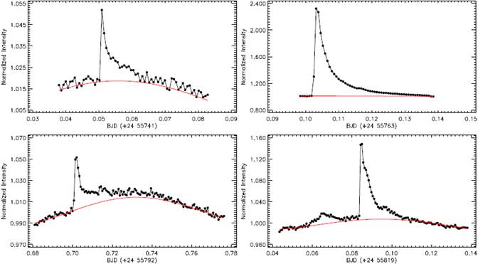
Fig. 5 Four different samples for the flare light variations are shown. In the figure, the filled circles represent the observations, while the (red) lines represent the synthetic light curve obtained from the light curve analysis, which was taken as the quiescent levels for each flare. The color figure can be viewed online. 

Taking into account that the luminosity parameter enters in the energy calculations as described by ^{Dal & Evren (2010}, ²⁰¹¹⁾, the equivalent duration parameter was computed for each flare, instead of its energy. According to the beginning and the end of a flare, the desired parameters, such as flare rise times (T _r ), decay times (T _d ), amplitudes of flare maxima, flare equivalent durations (P), were computed for each flare. The flare equivalent durations were computed by equation (2) taken from ^{Gershberg (1972)}:

P=∫[(Iflare-I0)/I0]dt (2)

where I ₀ is the flux of the star in the quiet state. As described above, the synthetic light curve derived by the light curve analysis was taken as I ₀. I _flare is the intensity observed at the moment of the flare. P is the flare-equivalent duration in the observing band. All the computed parameters are listed in Table 3 for these 149 flares. The general standard errors were computed by using the methods described by ^{Taylor (1997)} for the time scales such as flare rise and decay times.

Table 3 The flare parameters computed from KIC 12004834’s the available short cadence data in the Kepler mission database 

Tmax (BJD-2450000)	P (s)	Tr (s)	Td (s)	Tt (s)	Amplitude (Relative Flux)
55806.51506	0.762	58.846 ± 3.616	58.846 ± 3.616	117.692 ± 5.114	0.01180
55804.54459	0.471	58.846 ± 3.616	58.847 ± 3.616	117.693 ± 5.114	0.01221
55811.74873	0.896	58.847 ± 3.616	58.846 ± 3.616	117.693 ± 5.114	0.01720
55766.08239	0.745	58.848 ± 3.616	117.686 ± 5.114	176.534 ± 6.264	0.00989
55830.23880	1.240	58.845 ± 3.616	176.538 ± 6.264	235.383 ± 7.233	0.01713
55801.66075	1.066	117.702 ± 5.114	117.685 ± 5.114	235.386 ± 7.233	0.00827
55794.32581	1.117	58.855 ± 3.617	176.532 ± 6.263	235.387 ± 7.233	0.00929
55831.45798	1.880	117.700 ± 5.114	117.692 ± 5.114	235.392 ± 7.233	0.01391
55822.77794	1.137	58.846 ± 3.616	176.546 ± 6.264	235.392 ± 7.233	0.01338
55801.95704	2.098	58.846 ± 3.616	235.386 ± 7.233	294.233 ± 8.086	0.01416
55804.71215	1.290	117.684 ± 5.114	176.549 ± 6.264	294.233 ± 8.086	0.01001
55823.82889	1.051	58.846 ± 3.616	235.393 ± 7.233	294.240 ± 8.086	0.01032
55822.73912	1.633	117.692 ± 5.114	235.384 ± 7.233	353.076 ± 8.858	0.01343
55760.03465	0.632	58.848 ± 3.616	294.239 ± 8.086	353.087 ± 8.858	0.01071
55801.75679	2.621	58.838 ± 3.616	294.251 ± 8.087	353.088 ± 8.858	0.01381
55799.55611	1.312	117.702 ± 5.114	235.387 ± 7.233	353.089 ± 8.858	0.00642
55780.13399	1.711	117.703 ± 5.114	235.389 ± 7.233	353.092 ± 8.858	0.01102
55766.07149	0.848	117.704 ± 5.114	235.391 ± 7.233	353.094 ± 8.858	0.01050
55768.37983	2.922	58.857 ± 3.617	294.255 ± 8.087	353.112 ± 8.858	0.01705
55756.03029	1.168	117.687 ± 5.114	294.257 ± 8.087	411.944 ± 9.568	0.00935
55756.56293	1.245	117.696 ± 5.114	294.248 ± 8.086	411.944 ± 9.568	0.01079
55740.56791	2.973	117.696 ± 5.114	294.251 ± 8.087	411.947 ± 9.568	0.01556
55831.96472	4.468	58.846 ± 3.616	411.929 ± 9.568	470.775 ± 10.228	0.03456
55778.12332	2.165	117.694 ± 5.114	353.093 ± 8.858	470.787 ± 10.229	0.01238
55776.73927	1.898	117.695 ± 5.114	353.093 ± 8.858	470.788 ± 10.229	0.00963
55792.90704	6.883	117.694 ± 5.114	411.937 ± 9.568	529.631 ± 10.849	0.02718
55779.79002	9.266	117.694 ± 5.114	411.940 ± 9.568	529.634 ± 10.849	0.04237
55755.22928	3.861	176.552 ± 6.264	353.087 ± 8.858	529.640 ± 10.849	0.01210
55772.93588	0.849	117.704 ± 5.114	411.941 ± 9.568	529.644 ± 10.849	0.01032
55761.90026	1.219	117.704 ± 5.114	411.943 ± 9.568	529.648 ± 10.849	0.01217
55755.87908	1.132	294.248 ± 8.086	235.400 ± 7.233	529.648 ± 10.849	0.00573
55783.26307	0.793	58.856 ± 3.617	470.794 ± 10.229	529.650 ± 10.849	0.00322
55762.79935	1.244	117.704 ± 5.114	411.952 ± 9.568	529.655 ± 10.849	0.01132
55766.10282	2.214	294.247 ± 8.086	294.238 ± 8.086	588.485 ± 11.436	0.01453
55792.98265	2.377	117.693 ± 5.114	470.793 ± 10.229	588.486 ± 11.436	0.01164
55825.24424	2.172	117.700 ± 5.114	470.786 ± 10.229	588.486 ± 11.436	0.01260
55810.05753	1.166	176.557 ± 6.264	411.933 ± 9.568	588.489 ± 11.436	0.01357
55742.47985	1.287	176.545 ± 6.264	411.946 ± 9.568	588.490 ± 11.436	0.01300
55747.50593	1.506	117.696 ± 5.114	470.802 ± 10.229	588.498 ± 11.436	0.01536
55742.24282	3.543	294.241 ± 8.086	294.259 ± 8.087	588.500 ± 11.436	0.01447
55829.60128	2.781	117.692 ± 5.114	529.629 ± 10.849	647.322 ± 11.994	0.01256
55826.06293	3.057	176.546 ± 6.264	470.776 ± 10.228	647.323 ± 11.994	0.00379
55792.31311	1.336	176.540 ± 6.264	470.793 ± 10.229	647.333 ± 11.994	0.00897
55762.79186	3.297	117.686 ± 5.114	529.648 ± 10.849	647.334 ± 11.994	0.01830
55779.32482	2.116	117.703 ± 5.114	529.635 ± 10.849	647.337 ± 11.994	0.01469
55748.36688	1.896	235.392 ± 7.233	411.963 ± 9.568	647.355 ± 11.994	0.01075
55776.23933	3.682	117.694 ± 5.114	588.491 ± 11.436	706.185 ± 12.527	0.00924
55796.02792	3.817	117.703 ± 5.114	588.485 ± 11.436	706.188 ± 12.527	0.01597
55765.69482	5.587	235.408 ± 7.233	470.789 ± 10.229	706.197 ± 12.528	0.01827
55763.59627	1.525	117.704 ± 5.114	588.495 ± 11.436	706.199 ± 12.528	0.00532
55811.84817	9.222	176.539 ± 6.264	588.481 ± 11.436	765.020 ± 13.039	0.02482
55808.84242	3.326	176.548 ± 6.264	588.472 ± 11.436	765.020 ± 13.039	0.01629
55806.89444	2.641	294.241 ± 8.086	470.781 ± 10.229	765.022 ± 13.039	0.04012
55810.38923	3.032	176.548 ± 6.264	588.481 ± 11.436	765.029 ± 13.039	0.00910
55779.65108	6.755	176.551 ± 6.264	588.481 ± 11.436	765.031 ± 13.039	0.02747
55777.26170	2.436	58.847 ± 3.616	706.185 ± 12.527	765.032 ± 13.039	0.01427
55800.70583	1.053	176.549 ± 6.264	588.483 ± 11.436	765.032 ± 13.039	0.01235
55773.50393	2.461	235.407 ± 7.233	529.627 ± 10.849	765.034 ± 13.039	0.04477
55762.69582	2.510	58.839 ± 3.616	706.199 ± 12.528	765.038 ± 13.039	0.01041
55748.38868	3.771	117.704 ± 5.114	647.337 ± 11.994	765.042 ± 13.039	0.01522
55746.66405	1.236	117.704 ± 5.114	647.338 ± 11.994	765.043 ± 13.039	0.01060
55743.15553	2.308	353.098 ± 8.858	411.946 ± 9.568	765.043 ± 13.039	0.01575
55745.65597	2.618	117.705 ± 5.114	647.347 ± 11.994	765.052 ± 13.039	0.01126
55821.60644	2.042	294.230 ± 8.086	529.632 ± 10.849	823.862 ± 13.531	0.00904
55798.75171	4.518	58.838 ± 3.616	765.032 ± 13.039	823.871 ± 13.531	0.02078
55794.34352	4.924	58.856 ± 3.617	765.026 ± 13.039	823.882 ± 13.531	0.01618
55783.25353	3.925	235.388 ± 7.233	588.498 ± 11.436	823.886 ± 13.531	0.01514
55763.58673	4.125	176.551 ± 6.264	647.342 ± 11.994	823.893 ± 13.531	0.01013
55775.11139	3.272	117.704 ± 5.114	706.194 ± 12.528	823.897 ± 13.531	0.01310
55740.48481	2.590	294.250 ± 8.087	529.652 ± 10.849	823.902 ± 13.531	0.01744
55747.88464	3.972	58.857 ± 3.617	765.051 ± 13.039	823.908 ± 13.531	0.02227
55820.70669	11.448	176.546 ± 6.264	706.171 ± 12.527	882.717 ± 14.006	0.02987
55812.88346	5.447	58.855 ± 3.617	823.865 ± 13.531	882.720 ± 14.006	0.02041
55792.81781	3.461	411.937 ± 9.568	470.783 ± 10.229	882.720 ± 14.006	0.01339
55809.54465	3.030	117.693 ± 5.114	765.029 ± 13.039	882.722 ± 14.006	0.01444
55807.14032	3.450	411.934 ± 9.568	470.789 ± 10.229	882.723 ± 14.006	0.01147
55815.95868	2.639	58.856 ± 3.617	823.872 ± 13.531	882.728 ± 14.006	0.01146
55744.32436	4.279	176.553 ± 6.264	706.196 ± 12.528	882.749 ± 14.006	0.01569
55742.23055	5.768	117.705 ± 5.114	765.052 ± 13.039	882.757 ± 14.006	0.01393
55817.51569	6.776	117.701 ± 5.114	823.864 ± 13.531	941.565 ± 14.465	0.02661
55792.21979	1.686	176.541 ± 6.264	765.026 ± 13.039	941.567 ± 14.465	0.00954
55806.74527	3.401	176.548 ± 6.264	765.021 ± 13.039	941.569 ± 14.465	0.01014
55804.56094	2.295	176.539 ± 6.264	765.031 ± 13.039	941.571 ± 14.465	0.00944
55743.93339	1.965	176.553 ± 6.264	765.043 ± 13.039	941.597 ± 14.466	0.00956
55818.95147	5.622	58.846 ± 3.616	941.564 ± 14.465	1000.410 ± 14.911	0.02512
55820.43834	4.285	117.701 ± 5.114	882.718 ± 14.006	1000.419 ± 14.911	0.00997
55800.59413	2.617	117.702 ± 5.114	882.725 ± 14.006	1000.427 ± 14.911	0.01204
55773.99094	2.775	58.848 ± 3.616	941.585 ± 14.465	1000.433 ± 14.911	0.01211
55760.96984	3.584	117.696 ± 5.114	882.743 ± 14.006	1000.439 ± 14.911	0.01461
55777.94827	9.265	176.542 ± 6.264	823.897 ± 13.531	1000.439 ± 14.911	0.02508
55756.66238	4.502	176.552 ± 6.264	823.888 ± 13.531	1000.440 ± 14.911	0.01090
55755.86341	3.832	176.552 ± 6.264	823.897 ± 13.531	1000.449 ± 14.911	0.00772
55752.17713	3.504	176.553 ± 6.264	823.897 ± 13.531	1000.451 ± 14.911	0.01063
55803.99153	3.654	294.233 ± 8.086	765.022 ± 13.039	1059.254 ± 15.343	0.01084
55826.07315	3.786	176.546 ± 6.264	882.715 ± 14.006	1059.261 ± 15.343	0.00801
55741.05083	10.207	58.849 ± 3.616	1000.455 ± 14.911	1059.304 ± 15.343	0.03355
55805.48113	6.780	235.386 ± 7.233	882.724 ± 14.006	1118.109 ± 15.763	0.01629
55792.62642	8.534	353.090 ± 8.858	765.027 ± 13.039	1118.117 ± 15.763	0.02378
55751.93397	6.862	117.696 ± 5.114	1000.442 ± 14.911	1118.138 ± 15.763	0.03174
55765.32020	4.999	176.551 ± 6.264	941.589 ± 14.466	1118.140 ± 15.763	0.01279
55807.98013	4.321	117.702 ± 5.114	1059.261 ± 15.343	1176.963 ± 16.173	0.01249
55792.84574	5.480	176.549 ± 6.264	1000.423 ± 14.911	1176.972 ± 16.173	0.02244
55804.36682	5.572	235.386 ± 7.233	1000.417 ± 14.911	1235.803 ± 16.572	0.01366
55818.06535	18.899	117.692 ± 5.114	1118.111 ± 15.763	1235.803 ± 16.572	0.04024
55763.74271	5.420	235.399 ± 7.233	1000.445 ± 14.911	1235.845 ± 16.572	0.01580
55808.48143	6.886	294.241 ± 8.086	1000.415 ± 14.911	1294.656 ± 16.962	0.01014
55752.86099	2.487	470.793 ± 10.229	823.897 ± 13.531	1294.690 ± 16.962	0.01033
55748.43023	6.680	176.536 ± 6.264	1118.157 ± 15.764	1294.693 ± 16.962	0.01774
55757.40209	13.431	235.400 ± 7.233	1059.296 ± 15.343	1294.696 ± 16.962	0.02852
55740.24641	5.290	176.554 ± 6.264	1118.152 ± 15.764	1294.706 ± 16.962	0.01038
55755.23405	7.243	58.857 ± 3.617	1235.850 ± 16.572	1294.707 ± 16.962	0.02040
55799.53567	5.955	58.847 ± 3.616	1294.670 ± 16.962	1353.517 ± 17.343	0.02091
55759.69340	8.248	235.400 ± 7.233	1118.134 ± 15.763	1353.535 ± 17.344	0.01900
55748.56237	5.839	235.400 ± 7.233	1118.140 ± 15.763	1353.540 ± 17.344	0.01245
55746.72876	6.982	294.240 ± 8.086	1059.301 ± 15.343	1353.542 ± 17.344	0.01395
55759.69340	2.293	235.391 ± 7.233	1118.152 ± 15.764	1353.542 ± 17.344	0.00198
55820.42199	10.170	176.539 ± 6.264	1235.811 ± 16.572	1412.350 ± 17.716	0.01346
55797.44873	4.053	235.396 ± 7.233	1176.969 ± 16.173	1412.365 ± 17.716	0.01008
55807.03611	20.538	294.241 ± 8.086	1176.964 ± 16.173	1471.205 ± 18.082	0.03700
55791.63812	11.512	294.243 ± 8.086	1176.973 ± 16.173	1471.216 ± 18.082	0.02267
55746.15729	4.354	117.697 ± 5.114	1353.550 ± 17.344	1471.247 ± 18.082	0.01144
55806.00150	11.359	176.540 ± 6.264	1412.367 ± 17.716	1588.907 ± 18.791	0.02162
55787.89945	7.928	58.847 ± 3.616	1530.075 ± 18.440	1588.922 ± 18.791	0.00838
55768.84435	5.401	235.391 ± 7.233	1353.537 ± 17.344	1588.928 ± 18.791	0.01316
55833.09059	25.717	117.700 ± 5.114	1530.033 ± 18.440	1647.734 ± 19.136	0.07710
55819.06454	16.793	588.478 ± 11.436	1059.265 ± 15.343	1647.743 ± 19.136	0.02017
55766.87590	18.093	235.391 ± 7.233	1412.386 ± 17.717	1647.777 ± 19.136	0.03545
55773.95416	4.012	176.543 ± 6.264	1471.237 ± 18.082	1647.780 ± 19.136	0.01109
55790.05588	38.271	411.947 ± 9.568	1294.676 ± 16.962	1706.623 ± 19.475	0.16402
55816.58802	7.120	176.547 ± 6.264	1588.891 ± 18.791	1765.438 ± 19.807	0.01858
55793.88104	24.987	117.702 ± 5.114	1647.764 ± 19.136	1765.466 ± 19.808	0.11313
55826.02002	6.115	117.691 ± 5.114	1706.585 ± 19.475	1824.276 ± 20.135	0.01318
55827.89170	10.892	117.691 ± 5.114	1765.429 ± 19.807	1883.121 ± 20.457	0.02212
55819.08497	46.875	176.547 ± 6.264	1765.435 ± 19.807	1941.983 ± 20.774	0.14180
55780.39486	10.869	588.489 ± 11.436	1471.224 ± 18.082	2059.714 ± 21.395	0.01187
55765.45575	21.704	176.544 ± 6.264	1883.185 ± 20.457	2059.728 ± 21.395	0.04175
55822.75342	10.331	353.085 ± 8.858	2000.826 ± 21.087	2353.911 ± 22.872	0.01707
55828.63411	32.706	117.700 ± 5.114	2412.751 ± 23.156	2530.451 ± 23.714	0.04817
55821.43071	23.129	294.240 ± 8.086	2589.304 ± 23.988	2883.544 ± 25.314	0.01867
55756.89805	22.867	117.704 ± 5.114	2765.928 ± 24.793	2883.633 ± 25.315	0.03313
55763.10313	119.328	117.704 ± 5.114	2942.472 ± 25.572	3060.177 ± 26.078	1.31184
55764.80868	19.131	1059.301 ± 15.343	2059.729 ± 21.395	3119.030 ± 26.328	0.01630
55810.14130	28.083	176.548 ± 6.264	3118.961 ± 26.327	3295.509 ± 27.062	0.02015
55795.62606	59.471	117.703 ± 5.114	3236.660 ± 26.820	3354.362 ± 27.303	0.05526
55822.11727	32.769	235.392 ± 7.233	3177.782 ± 26.575	3413.175 ± 27.541	0.02822
55795.07436	37.409	353.089 ± 8.858	3589.768 ± 28.245	3942.857 ± 29.601	0.04263
55792.70202	36.928	176.541 ± 6.264	3766.321 ± 28.931	3942.862 ± 29.601	0.04881
55766.71856	117.197	235.391 ± 7.233	4119.463 ± 30.257	4354.854 ± 31.109	0.11637
55741.94107	52.968	1059.303 ± 15.343	4296.050 ± 30.899	5355.353 ± 34.498	0.02498

The distributions of flare equivalent durations on a logarithmic scale versus flare total durations were modelled by the One Phase Exponential Association (hereafter OPEA) defined by equation (3), using the SPSS V17.0 (^{Green et al. 1999}) and GrahpPad Prism V5.02 (^{Dawson & Trapp 2004}) software:

y = y0 + (Plateau - y0) × (1 - e-k × x) (3)

where y is the flare equivalent duration, x is the flare total duration. According to the description of ^{Dal & Evren (2010)}, the most important parameter in this equation is the P lateau term to reveal the flare behavior of a star. Following three different methods described by ^{D’Agostino & Stephens (1986)}, the probability values (p − value) were calculated to test the quality of the fit. The p − value was found to be < 0.001 in all the methods. The derived OPEA model is shown in Figure 6 together with the observed flare equivalent durations. The parameters computed from the model are listed in Table 4.

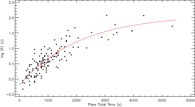
Fig. 6 The OPEA model derived from 149 flares detected in the available short cadence data of KIC 12004834 is shown. In the figure, the filled circles represent the calculated log(P) values from observations, while the red line represents the OPEA model. The color figure can be viewed online. 

Table 4 The OPEA model parameters derived by using the least-squares method 

Parameter	Value
Y 0	−0.197 ± 0.081
Plateau	2.093 ± 0.236
K	0.00048 ± 0.00010
Tau	2098.68
Half − life	1454.7
95% Confidence Intervals
Y 0	−0.355 to −0.038
Plateau	1.630 to 2.556
K	0.00029 to 0.00067
Tau	1497.65 to 3505.49
Half − life	1038.09 to 2429.82
Goodness of Fit
R 2	0.7628
p − value (D’Agostino-Pearson)	0.0001
p − value (Shapiro-Wilk)	0.0001
p − value (Kolmogorov-Smirnov)	0.0005

In contrast to the known UV Ceti flare stars, KIC 12004834 is a binary system. It is well known that the flare events are generally random phenomena. To test this situation for a close binary like KIC 12004834, we calculated the phase distribution of the flares, depending on the orbital period of the system. The phase distribution is shown in Figure 7. In the figure, the distribution of the total number of flares computed in phase intervals of 0.05, for all 149 flares is shown.

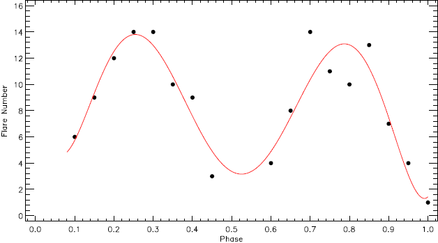
Fig. 7 The distribution of flare total number in each phase interval of 0.05, plotted versus phase for 149 flares. The color figure can be viewed online. 

We also derived the flare energy spectrum (^{Gershberg 1972}) for KIC 12004834. Like for the OPEA model, we again used the flare equivalent duration instead of the flare energy. To derive the flare energy spectrum, the cumulative flare frequencies were computed for 149 flares, and then, its distribution was derived in order to compare KIC 12004834 to its analogues. The obtained cumulative flare frequency distribution and its models are shown in Figure 8.

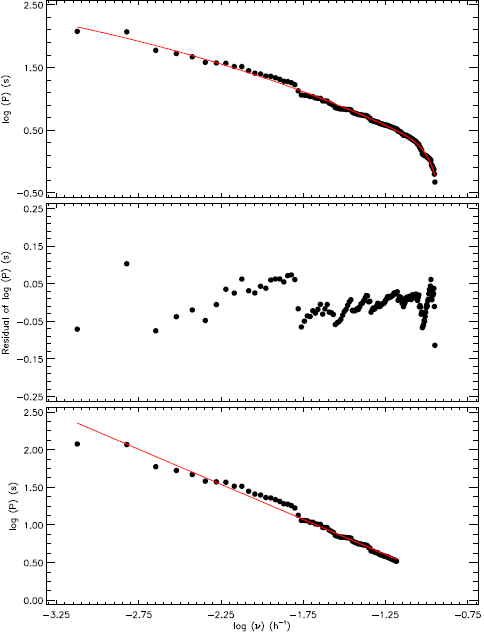
Fig. 8 Cumulative flare frequencies and model computed for 149 flares obtained from KIC 12004834. In the upper panel, the variation of the flare equivalent durations versus the cumulative flare frequency is shown, while the residuals obtained from the model are shown in the middle panel. The bottom panel shows the linear part of the flare energy spectrum and its linear representation. The color figure can be viewed online. 

In the literature there are two other flare frequency descriptions. Contrary to ^{Gershberg (1972)}, ^{Ishida et al. (1991)} described the flare frequencies N ₁ and N ₂, a flare number and a total flare-equivalent duration emitting per hour, respectively. In this study, we detected 149 flares from the available observations lasting 89.19 days. We computed the frequencies by equations (4) and (5) (^{Ishida et al. 1991}):

N1 = Σnf / ΣDT (4)

N2 = ΣP / ΣDT (5)

where Σnf is the total flare number, ΣDT is the total observing duration, and ΣP is the total equivalent duration. We found that the N ₁ frequency is 0.070 h^-1, while the N ₂ frequency is 0.62 second/hour for KIC 12004834. It should be noted that the N ₂ frequency is a unitless parameter, because the unit of ΣDT is time as well as the unit of ΣDT. However, the N ₂ frequency is given in units of second/hour to facilitate the reading of the manuscript.

3. Results and discussion

We analysed the light curve and (O − C) residuals of the system for the first time in the literature. The mass ratio of the system (q) was found to be 0.743 ± 0.001, while the inclination (i) was found to be 75º.89 ± 0^◦.03. This inclination (i) value is in agreement with the inclination (i) value of 72º.47 given by ^{Coughlin et al. (2011)}. The mass of the primary component was found to be 0.64M⊙ with a radius of 0.70R⊙, while it was found to be 0.57M⊙ for the secondary component with a radius of 0.65R⊙. Although these parameters are a bit larger than those found by ^{Coughlin et al. (2011)}, it can be assumed that they are in agreement. In addition, these values indicate that KIC 12004834 is a simple close binary system. Indeed, the possible semi-major axis was found to be as small as 1.84R⊙ (≈ 0.0086 AU), which indicates that there must be a distance of 0.49R⊙ between the surfaces of the components. In this case, it is possible that each component can trigger the magnetic activity of the other.

If being in a very close binary affects the chromospheric patterns of the active component, we should see an effect: an increase of the flare frequency or of the Plateau value. KIC 12004834 was continuously observed over 89.19 days from JD 24 55739.83568694 to JD 24 55833.27789066, and we detected 149 flare events. The flare frequency N₁, the general flare number per an hour, was found to be 0.070 h ^-1, while the flare frequency N₂, the averaged flare energy per an hour, was computed as 0.62 second/hour. However, according to these results, KIC 12004834 did not show a high magnetic activity, not at the expected level.

Comparing the target to similar systems, we can easily notice that like KIC 12004834, both FL Lyr and KIC 9761199 are binary systems, but with high level chromospheric activity. Indeed, the flare frequencies of FL Lyr were recently found to be N₁ = 0.41632 h⁻¹ and N₂ = 0.00027 by (^{Yoldaş & Dal 2016}). However, the radii of the FL Lyr components were given as R1=1.283R⊙, R2=0.963R⊙ with a semi-major axis of a=9.17R⊙ by ^{Eker et al. (2014)}. In the case of KIC 9761199, ^{Yoldaş & Dal (2017)} found the P lateau value as 1.951 s, while the flare frequencies, N₁ and N₂, were found to be 0.01351 h ^-1 and 0.00006, respectively. The authors computed the masses of the primary and secondary components as 0.57M⊙, 0.39M⊙, and the radii of the components as 0.62R⊙ and 0.56R⊙ with a semi-major axis of a=5.16R⊙. According to these results, if being a close binary affects the surface magnetic activity, KIC 12004834 should exhibit more frequent or more powerful flares than FL Lyr. On the other hand, according to Dal & Evren (2011); ^{Dal (2012)}, it is a controversial topic whether the flare frequencies are an indicator of flare activity level, or not. There is one more parameter that may be taken an indicator for the flare activity level, which is the Plateau value. The Plateau value was found to be 2.093±0.236 s from the OPEA model of KIC 12004834. However, Yoldaş & Dal (2016) found the Plateau value as 1.232±0.069 s for FL Lyr. According to these results, the activity level of KIC 12004834 is nearly two times higher than FL Lyr, as expected. With an increasing number of eclipsing binaries with a flaring component, we may determine which parameter is real indicator for the flare activity level.

Using the regression calculations, the half−life value was found to be 1454.7 s from the OPEA model for KIC 12004834. In the case of FL Lyr, it is 2291.7 s (^{Yoldaş & Dal 2016}). This means that a flare occurring on FL Lyr can reach the maximum energy level when the flare total duration reaches 38 minutes, while it takes 24.245 minutes for KIC 12004834. Moreover, the maximum flare rise time (T _r ) obtained from the flares of KIC 12004834 was found to be 1059.303 s, while the maximum flare total time (T _t ) was found to be 5355.050 s. However, these values are T _r = 5179.00 s and T _t = 12770.62 s for FL Lyr. As a result, the FL Lyr flare time scales are obviously larger than those obtained from KIC 12004834, which is in agreement with the results found by Dal & Evren (2011); ^{Dal (2012)} for single flare stars of type dMe.

However, there is one more controversial feature of KIC 12004834, which is stellar spot activity. During the analysis process, we recognised that the synthetic curve derived without any stellar spot does not fit the observations around phase 0.27. Because of this, the results of the light curve analysis point to the presence of stellar spot activity on one of the components. Considering the temperatures of the components we assumed that the flare activity is a sinusoidal variation caused by the rotational modulation due to the stellar cool spots. Indeed, this sinusoidal variation could be easily modelled with a cool spot on the primary component as seen in the 3D model of Roche geometry shown in Figure 4. However, the analyses indicated that the location of the spot is not changed on the primary component along 89.19 day despite the presence of high level flare activity. Considering the rapid variation in the flare behaviour, a stable spotted area on the component is very interesting. According to ^{Hall et al. (1989)} and ^{Gershberg (2005)}, it is well known that the spotted areas on the active components of some RS CVn binaries can keep their shapes and locations for as long as two years. Therefore, the behavior of the cool spot activity observed for KIC 12004834 is not inconsistent with the stellar spot activity phenomenon.

In addition, considering the distribution of the total flare number in each phase interval of 0.05, it is noticed that the flares tend to occur in two specific phases, 0.25 and 0.75, as seen in Figure 7. Since the spotted area is seen around phase 0.27, the behavior of the flare activity of this close binary system KIC 12004834 can be understood.

At this point, one can question whether the sinusoidal variation out-of-eclipses is really caused by the stellar spots. In the literature, ^{Tran et al. (2013)} found a way to obtain the sign of the spot activity. They demonstrated that the spot activity remarkably affects the variations of the (O − C) residuals, especially for the (O − C)_II residuals. ^{Tran et al. (2013)} reported that the stellar spot activity occurring on the active component causes the (O − C)_II residuals of both the primary and secondary minima to vary synchronously in a sinusoidal manner, but in opposite directions. We could not determine the minima times from the Kepler long cadence data because the orbital period of KIC 12004834 is short, 0^d.262317. However, we determined all the minima times from the available short cadence data. In the Kepler Mission Database, the short cadence data of observations are covered over 100 days. Because of this, the sinusoidal variation cannot be properly seen. On the other hand, we determined that the minima times computed from the primary and the secondary minima are separated from each other. This is enough evidence for the spot presence on one component.

We wish to thank the Turkish Scientific and Technical Research Council for supporting this work through grant No. 116F213. We thank the referee for useful comments that have contributed to the improvement of the paper. We also thank Dr. O. Özdarcan for the useful scripts that have supported us, providing an easy way to solve hard calculations.