1. Introduction

The exploration of the Kuiper Belt Objects (KBOs) is an important step to improve the theories of the formation of the Solar System, since these bodies probably preserved material from the earlier Solar System (^{Luu & Jewitt 2002}). Furthermore, due to the large distance to these bodies from the Sun, the development of new technologies and techniques for their exploration is required.

A few years ago these objects were thought to be single bodies with no atmosphere, except for Pluto. However, with the advances of observational techniques, it was discovered that several of these bodies are orbited by one or more small moons, like Haumea, Makemake, and Quaoar³. Another interesting point is that the New Horizons spacecraft, when passing by Pluto, discovered that Pluto has signs of recent surface activity (less than 10 million years old) (^{Moore et al. 2016}). This fact can be an indication that other KBOs with sizes comparable to Pluto could also present recent geological activity. One example of this possibility is the potential presence of cryovolcanism in Quaoar (^{Barucci et al. 2015}). However, due to the large distance of the KBOs from the Sun, observational data were not enough to significantly improve our knowledge about these bodies, to carry out comparative planetology. Spacecraft missions to one or more of these bodies beyond Pluto are necessary to provide us with more detailed features of the KBOs. The present paper searches for optimal trajectories to (136108) Haumea, (136472) Makemake, and (50000) Quaoar. These three bodies were chosen as targets because they are good representatives of the KBOs and they can also be classified as Trans-Neptunian Objects (TNOs). Haumea and Makemake were recognized by the International Astronomical Union (IAU) as dwarf planets, but Quaoar is just a candidate to this classification. Haumea is probably the most intriguing of the TNOs, because it is a triaxial ellipsoid with fast rotation (3.9154 h), possesses two moons, Namaka and Hi’iaka, and a recently discovered ring (^{Ortiz et al. 2017}). The thin layer of carbon depleted ice that surrounds the rocky core of Haumea is another important characteristic of this dwarf planet (^{Pinilla-Alonso et al. 2009}).

Makemake is the third largest TNO, after Pluto and Eris. It also has a recently discovered moon, which has no official name yet, and its general designation is “S/2015 (136472) 1” (^{Parker et al. 2016}). Quaoar also has a small moon, named Weywot. This moon seems to be in an eccentric orbit. Like Haumea, Quaoar has a rocky core covered by a thin layer of ice, but differently from Haumea, Quaoar has a high density and probably its core is entirely formed by silicate material (^{Fraser et al. 2013}). Then, Quaoar probably is the densest TNO, which makes it a good target for spacecraft exploration. Table 1 presents some orbital and physical characteristics of Haumea (^{Ragozzine & Brown 2009}; ^{Ortiz et al. 2017}), Makemake (^{Brown 2013}; ^{Parker et al. 2016}), and Quaoar (^{Fraser et al. 2013}). The values of the semi-major axes (a), eccentricities (e) and inclinations (I) are approximate. The inclinations are given with respect to the ecliptic plane. Table 1 also presents the masses (m), densities (ρ), and the moons of these bodies.

We analyzed the dates of launch in the 2023-2034 interval. The only exception was direct flight to Haumea with launch in 2058. The optimal transfer trajectories in terms of the minimum fuel consumption were found. Instead of the fuel consumption an equivalent parameter was considered, namely the total ΔV, which is the sum of the launch V in the low Earth parking orbit and all necessary ΔV s during the flight.⁴ This was done considering various possible transfer schemes for the given launch windows assuming that the dwarf planets will be flown by without capture. If capture is required for these specific trajectories, a new optimization should be made taking into account the capture maneuver. Most of the transfer schemes considered include various gravity assists of the planets, which lowers the fuel consumption and/or shortens the time of flight. Furthermore, multi-body missions are more interesting from the scientific point of view, since scientific data could be acquired during the flybys. However, since the limited time of flight is considered, the number of bodies in a single trajectory may be limited. Thus, the number of the planets was maximized for trajectories with 20 years of total time of flight, leaving a smaller number of planets for trajectories with total time of flight less than 20 years. The main difficulty in the design of these trajectories is to find feasible combinations of planets, within the proposed time interval, in a realistic time of flight. Some combinations are not always possible. For example, the combination used by the mission of the Voyager 2 (^{Kohlhase & Penzo 1977}), Earth-Jupiter-Saturn-Uranus-Neptune-Outer space, cannot be reproduced in this century anymore. This technique was widely used in missions to the outer planets and outer space, such as in the Voyager 1 (^{Kohlhase & Penzo 1977}), with the scheme E-J-S-Outer space, Galileo (^{D’Amario et al. 1982}), with the scheme E-V-E-E-A-A-J, Ulysses (^{Wenzel et al. 1992}), with the scheme E-A-DV-E-A, Cassini (^{Peralta & Flanagan 1995}), with the scheme E-V-V-E-A-J-S, and the New Horizons (^{Guo & Farquhar 2005}), with the scheme E-A-J-P-Kuiper Belt, where E, V, J, S, U, N, P, A stand for Earth, Venus, Jupiter, Saturn, Uranus, Neptune, and anăasteroid, respectively.ăDV means a deep space propulsive maneuver. All of these schemes, except E-V-V-E, which areăpossible for launch in 2023-2034 areăanalyzed in this paper. Also transfer schemes E-V-E-E-S andăE-V-E-DV-E-S are considered.

The method of patched-conics is a well-known technique and was used for the planning of several interplanetary missions (^{Kohlhase & Penzo 1977}; ^{D’Amario et al. 1982}; ^{Sukhanov 1999}; ^{Strange & Longusky 2002}; ^{Solórzano et al. 2008}). The description of the method can be found in several publiccations, like ^{Escobal (1968)}. The transfer trajectories shown here can be useful for future missions to Haumea, Makemake, and Quaoar, which are important targets in the future exploration of the Solar System.

2. Methodology

The patched-conic technique, making close approaches of the spacecraft to the planets of the Solar System, is used to generate sets of trajectories between Earth and Haumea, Makemake, and Quaoar. The software implemented to solve this problem generates all possible trajectories between the Earth and the final destination, choosing as optimal trajectory the one with the minimum ΔV required, for a given a launch window. This means that extended launch, swingby, and arrival time windows, up to a few and sometimes several months, were specified and optimal transfers within the windows were sought for. Thus, the trajectories found are optimal from the fuel consumption point of view. As mentioned above, this minimum ΔV does not consider the ΔV required to place the spacecraft in a close orbit around the dwarf planet, since the arrival velocity is too high: it can vary from 10 km/s to 22 km/s in trajectories with 10 to 20 years of time of flight, as shown in the next section. Then, the minimum to generate the optimal trajectory comprises the launch ΔV and mid-course maneuvers. The orbits of the planets were calculated using the JPL DE405 ephemerides. Orbital elements of the dwarf planets were taken from the Edward Bowell’s Asteroid Orbital Elements Database and then numerically propagated to the arrival time. In order not to make the transfers too long the time of flight was limited by some values and the optimal transfers (i.e. transfers with minimal total ΔV) for that limited time of flight were calculated.

3. Results

All types of the trajectories found for each of the dwarf planets are presented in this section. First, the direct Earth to the dwarf planet transfer is considered. Then transfers including gravity assists of the planets are considered, which increases the space-craft velocity and decreases the launch ΔV. To decrease the launch ΔV, the classical combination of multiple gravity assist maneuvers in Earth and Venus are used, such as EVEE (Earth-Venus-Earth-Earth) and EVEdvE (Earth-Venus-Earth-deep space maneuver-Earth). However, these maneuvers may increase the total time of flight, because the duration of the EVEE and EVEdvE maneuvers is about 3.5 years, and, consequently, it may not be possible to find transfer trajectories with less than 20 years and a total ΔV less than 10 km/s. This value for the total ΔV is a limit in the present research, when searching for transfers in the 2023-2034 interval and 2058 for the direct flight to Haumea.

The last planet in the way to the dwarf planet is the one responsible for changing the orbital inclination of the spacecraft, since all dwarf planets have considerable inclination to the ecliptic plane, as seen in Table 1. This gravity assist maneuver is used also to minimize the cost of the inclination change, which is a very expensive maneuver if made using the fuel consumption. The types of transfers are ordered by the number of the planets involved, beginning with the direct transfer. The name of the trajectory indicates the first letter of the planets involved and the constraint in the time of flight, where “nc” stands for “no constraints”. For example, the trajectory EJH60y is a type B trajectory, representing the Earth to Haumea passing by Jupiter with a maximum of 60 years of time of flight. It is worth mentioning that not all types of trajectories are possible for all the dwarf planets. The types of trajectories are the following:

If there is more than one transfer of the same type, it will be numbered along the type of the transfer, e. g., A1, A2, and so on.

Since Haumea, Makemake, and Quaoar are KBOs, all transfer trajectories pass by the main asteroid belt. This makes it possible to encounter and observe a main belt asteroid (or asteroids), increasing the scientific output of the mission. However, since the trajectories with smaller time of flight pass through the main belt with high velocity, the additional ΔV required to encounter an asteroid could increase too much the total ΔV. This is why only the 20-year trajectories include possible encounters with the asteroids. The results are shown for each individual target. The next three subsections give the main results for the trajectories to Haumea (Table 2), Makemake (Table 3), and Quaoar (Table 4). Plots of some of the trajectories are also shown, to illustrate the transfers. The results are summarized in the last subsection. All the dates presented in the results are in format dd.mm.yyyy, where dd = day, mm = month and yyyy = year.

3.1. Transfers to Haumea

Since inclination of the Haumea orbit to the ecliptic plane is about 28.2 degrees, the direct transfer to this body would have its minimum fuel consumption if the spacecraft reaches Haumea at the node line, i.e., the intersection of the Haumea orbital plane with the ecliptic plane. The reason is the very high cost of maneuvers to change the inclination of the spacecraft orbit. Then, the first trajectory presented in Table 2, the EHnc (type A), is a direct transfer using the best scenario, with the launch date of (23.01.2058) and the arrival date of (11.03.2100), just when Haumea is passing by the line of nodes. In Table 2, V_L is the launch ΔV, V_A is the arrival velocity, ΔV_T is the total ΔV, and TOF is the time of flight. Figure 1 shows the trajectory for the direct transfer.

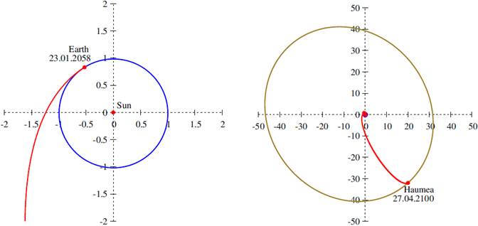
Fig. 1 Optimal transfer trajectory (red) to Haumea in the ecliptic plane. The orbit of the Earth is shown in blue and the orbit of Haumea in olive. The departure from the Earth is shown on the left and the whole trajectory on the right. The distances are given in astronomical units. The color figure can be viewed online. 

The addition of the Jupiter swingby during the Earth to Haumea transfer allows to decrease the launch V , the arrival velocity, the total ΔV and the time of flight, if compared with the EHnc transfer with launch in 2058. In the EJH60y transfer, the total ΔV decreased from 8.27 km/s to 6.84 km/s, a difference of 1.43 km/s compared to the transfer EHnc. The decrease of the ΔV at launch is 1.43 km/s, almost the same as the total ΔV. The same proportion was followed by the arrival velocity, which has a decrease of 1.43 km/s. This indicates that the arrival velocity is more sensitive to variations in the time of flight, since the arrival time for the EHnc transfer is almost the same as for the EJH60y transfer.

Figure 2 shows the EJH20y transfer trajectory, and Figure 3 shows the EJH10y trajectory. The latter transfer is the best solution found for the relatively short time of flight, since the total ΔV was kept under 10 km/s.

Fig. 2 Optimal transfer trajectory (red) to Haumea in the ecliptic plane, including a Jupiter swingby. The orbits of the planets are shown in blue, and the orbit of Haumea in olive. The Earth to Jupiter flight is shown on the left and the whole transfer trajectory on the right. The distances are given in astronomical units. The total time of flight was constrained to 20 years. The color figure can be viewed online. 

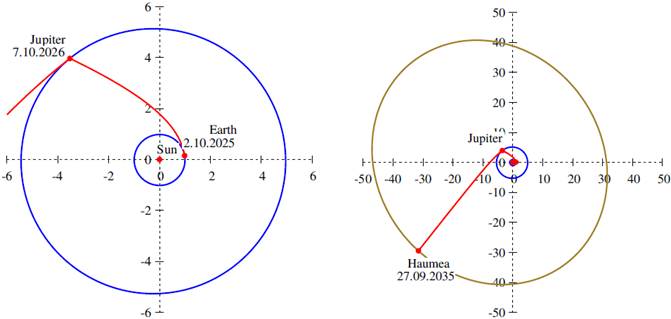
Fig. 3 The same as in Figure 2, but with a 10-year time of flight. The color figure can be viewed online. 

The launch ΔV can be reduced by means of the EVEE or EVEdvE maneuver. As an example, Figure 4 shows the EVEEJH20y transfer for launch in 2023. If we compare this transfer with the EJH20y shown in Table 2, there is decrease in the total ΔV of 1.43 km/s and decrease of 3.69 km/s in the launch ΔV. However, since the spacecraft passed by more planets in the same period of time as the EJH20y transfer, the mid-course velocity increment of the spacecraft in EVEEJH20y is larger than the one for the EJH20y situation, leading to a 1.93 km/s higher arrival velocity.

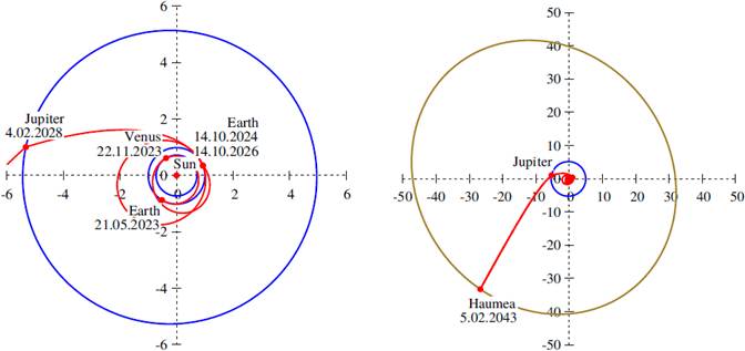
Fig. 4 Optimal transfer trajectory (red) to Haumea in the ecliptic plane, including the EVEE maneuver and the Jupiter swingby. The orbits of the planets are marked in blue, and the orbit of Haumea in olive. The departure from the Earth is shown on the left and the whole trajectory on the right. The distances are given in astronomical units. The total time of flight is constrained to 20 years. The color figure can be viewed online. 

The EVEdvEJH20y transfer trajectory that uses the deep space maneuver is shown in Figure 5. The use of the deep space maneuver between the two Earth swingbys leads to a small decrease of the total ΔV, namely, of 0.11 km/s. We used the EVEd-vEJH20y transfer to search for the asteroids that could be encountered in the 20-year trajectory. Just one asteroid that could be reached during the transfer with an additional ΔV < 0.5 km/s was found. This asteroid is (11023) 1986 QZ. Figure 6 includes the orbit of the asteroid, the date of the encounter, and the trajectory EVEdvEJH20y. Characteristics of the original EVEdvEJH20y transfer and the transfer with the asteroid encounter are shown in Table 2, as E3 and E4. The additional ΔV necessary for the asteroid is 0.10 km/s.

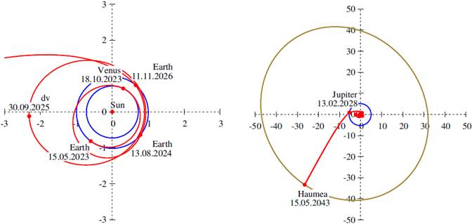
Fig. 5 Optimal transfer trajectory (red) to Haumea in the ecliptic plane, including the EVEdvE maneuver and the Jupiter swingby. The orbits of the planets are marked in blue and the orbit of Haumea in olive. The departure from the Earth is shown on the left and the whole trajectory on the right. The distances are given in astronomical units. The total time of flight is constrained to 20 years. The color figure can be viewed online. 

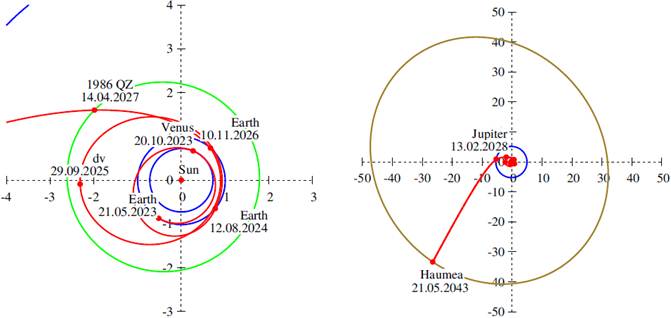
Fig. 6 Optimal transfer trajectory (red) to Haumea in the ecliptic plane, including the EVEdvE maneuver, the (11023) 1986 QZ asteroid encounter, and the Jupiter swingby. The orbits of the planets are marked in blue, the orbit of the asteroid in green, and the orbit of Haumea in olive. The departure from the Earth is shown on the left and the whole trajectory on the right. The distances are given in astronomical units. The total time of flight is constrained to 20 years. The color figure can be viewed online. 

The existence of launch windows with the Saturn gravity assist in the 2023-2034 interval allows another possibility of transfers to Haumea using the EVEdvE maneuver. However, compared with the similar combination, but using Jupiter instead of Saturn, all transfers that involve Saturn have a larger total ΔV, as can be seen in Table 2. There are also launch windows with Uranus swingby after Jupiter, but they also have a large total V compared with other trajectories with the same time of flight, as also shown in Table 2. Transfer trajectories passing by Uranus exceed our limit of 10 km/s in all transfers that have total time of flight smaller than 25 years.

3.2. Transfers to Makemake

Characteristics of the transfers to Makemake are given in Table 3, where ΔV_L is the launch ΔV, V_A is the arrival velocity, ΔV_T is the total ΔV, and TOF is the time of flight. Makemake is three astronomical units farther from the Sun than Haumea. This fact, associated with an inclination larger by one degree, makes the fuel consumption larger. It can be seen, from the total ΔV for the transfer trajectories to Makemake, that, for all the transfers, the fuel expenditures are slightly larger than the ones for the transfers to Haumea. Comparing Table 2 with Table 3, one can see that the same type of trajectory has larger values of the total ΔV for Makemake. As an example, for the transfer type A, which is a direct transfer to the body, the total ΔV is 8.24 km/s for the Earth-Haumea flight and 8.33 km/s for the Earth-Makemake flight. Transfer A1 for Makemake is shown in Figure 7.

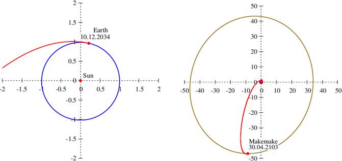
Fig. 7 Optimal transfer trajectory (red) to Makemake in the ecliptic plane. The orbit of the Earth is marked in blue, and the orbit of Makemake in olive. The departure from the Earth is shown on the left and the whole trajectory on the right. The distances are given in astronomical units. The color figure can be viewed online. 

Similarly to what occurs for Haumea, transfer trajectories using the Jupiter swingby spend less total ΔV compared to transfers using the Saturn swingby, as is shown in Table 3. Very large variations in the costs for different types of trajectories are noted. As an example of this variation, note that the B3 type of transfer (Earth-Jupiter-Makemake) has a total ΔV of 10.43 km/s, which is almost half of the total ΔV for the transfer C3 (Earth-Saturn-Makemake), which is 17.72 km/s. Both transfers considered a time of flight of 10 years. The transfer B3 is shown in Figure 8.

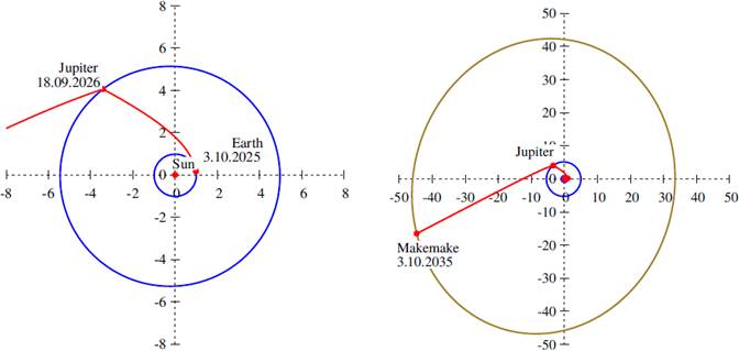
Fig. 8 Optimal transfer trajectory (red) to Makemake in the ecliptic plane, including a Jupiter swingby. The orbits of the planets are marked in blue, and the orbit of Makemake in olive. The distances are shown in astronomical units. The total time of flight is constrained to 10 years. The color figure can be viewed online. 

However, if we consider the EVEdvE maneuver before the Saturn or Jupiter swingby, our simulations show that Saturn is more efficient in terms of reducing the total ΔV. In the same way as transfers to Haumea, a 20-year transfer is feasible if a mission passing by multiple bodies is designed, having the total ΔV around 10 km/s. Therefore, regarding the search of asteroids that can be encountered in the way from Earth to Makemake, the F2 transfer (EVEdvESM20y) is chosen. This transfer is shown in Figure 9. Three asteroids can be encountered with an additional ΔV of less than 1 km/s, which is not too much considering the scientific gains of the mission. The asteroids are: (96168) 1981 ER23, with an additional ΔV of only 0.04 km/s; (12062) 1998 FB10, with an additional ΔV of 0.12 km/s; and (135420) 2001 UT44, with additional ΔV of 0.14 km/s. The transfer trajectories reaching these three asteroids are shown in Figures 10, 11, and 12, respectively.

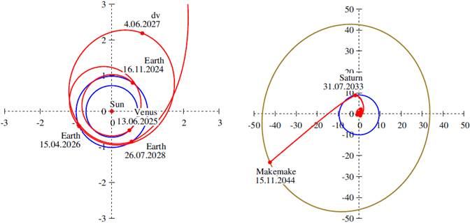
Fig. 9 Optimal transfer trajectory (red) to Makemake in the ecliptic plane, including the EVEdvE maneuver and the Saturn swingby. The orbits of the planets are marked in blue, and the orbit of Makemake in olive. The departure from the Earth is shown on the left and the whole trajectory on the right. The distances are given in astronomical units. The total time of flight is constrained to 20 years. The color figure can be viewed online. 

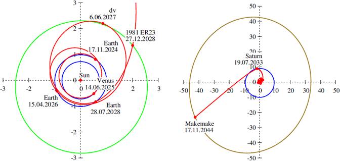
Fig. 10 Optimal transfer trajectory (red) to Makemake in the ecliptic plane, including the EVEE maneuver, the Jupiter swingby and the (96168) 1981 ER23 asteroid encounter. The departure from the Earth is shown on the left and the whole trajectory on the right. The orbits of the planets are marked in blue, the orbits of the asteroid in green, and the orbit of Makemake in olive. The distances are given in astronomical units. The total time of flight is constrained to 20 years. The color figure can be viewed online. 

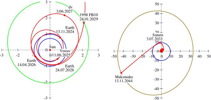
Fig. 11 Transfer type F4. The same as in Figure 10, but with the (12062) 1998 FB10 asteroid encounter. The color figure can be viewed online. 

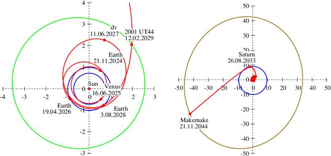
Fig. 12 Transfer type F5. The same as in Figure 10, but with the (135420) 2001 UT44 asteroid encounter. The color figure can be viewed online. 

3.3. Transfers to Quaoar

Characteristics of the transfers to Quaoar are given in Table 4, where ΔV_L is the launch ΔV, V_A is the arrival velocity, ΔV_T is the total ΔV, and TOF is the time of flight. The orbit of Quaoar has a semi-major axis of 44 astronomical units, and this number places its orbit between the orbits of Haumea and Makemake, because the eccentricity of Quaoar is low. However, the orbital inclination of Quaoar to the ecliptic plane is 8 degrees. In this case, due to the lower inclination compared to Haumeaand Makemake, all transfer trajectories from Earth to Quaoar have fuel consumption, expressed by the total ΔV, smaller than the ones required for the transfers to Haumea or to Makemake. This fact can be seen if Tables 2, 3, and 4 are compared with each other. To exemplify this fact, the transfer using a Jupiter swingby and considering a 10-year time of flight can be used for comparisons. In the case of Haumea, this transfer requires a total ΔV of 9.98 km/s to be executed. For Makemake, the value is ΔV = 10.43 km/s; while for Quaoar it is ΔV= 8.34 km/s. Since, in this paper, we fixed a limit of 10 km/s for the total ΔV , it is possible to obtain a transfer to Quaoar with a flight time of 8 years and total ΔV = 9.73 km/s. This means that Quaoar can be reached in less than a decade of flight, which makes it a very convenient target. Figure 13 shows the 8-year Earth-Jupiter-Quaoar transfer.

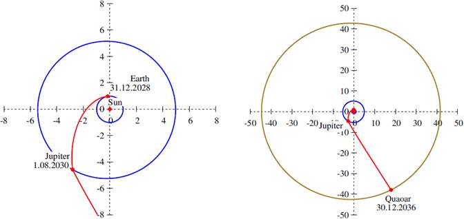
Fig. 13 Optimal transfer trajectory (red) to Quaoar in the ecliptic plane, including the Jupiter swingby. The orbits of the planets are marked in blue and the orbit of Quaoar in olive. The departure from the Earth is shown on the left and the whole trajectory on the right. The distances are given in astronomical units. The time of flight is 8 years. The color figure can be viewed online. 

In the case of Quaoar, similarly to that of Haumea, all the Earth-Jupiter-Quaoar transfers are more efficient, in terms of total ΔV, than the Earth-Saturn-Quaoar transfers. This fact can be seen in Table 4. Similarly to what occurred for Haumea, the EVEdvE transfer is more efficient if combined with a Jupiter swingby. Therefore, the transfer E1 (EVEdvEJQ20y) is used to search for possible as teroids encounters in the way from Earth to Jupiter. In this case, although the total ΔV of this transfer is 6.13 km/s, and this fact makes it possible to find transfers of the same type in shorter times of flight, we decided to keep the limit of 20 years of time of flight to allow the reader to compare this type of transfer for the three bodies Haumea, Makemake, and Quaoar. The transfer E1 is shown in Figure 14 as an example.

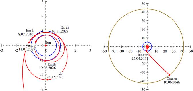
Fig. 14 Optimal transfer trajectory (red) to Quaoar in the ecliptic plane, including the EVEdvE maneuver and the Jupiter swingby. The orbits of the planets are marked in blue and the orbit of Quaoar in olive. The departure from the Earth is shown on the left and the whole trajectory on the right. The distances are given in astronomical units. The total time of flight is constrained to 20 years. The color figure can be viewed online. 

Two asteroids can be reached with an additional ΔV of around 1 km/s, a value that is not too large. The asteroid (155385) 1993 UO6 can be reached with an additional V of only 0.26 km/s, while the asteroid (64378) 2001 UE122 can be visited with an additional ΔV of 1.13 km/s. The transfers that contain the passage by these asteroids are shown in Figures 15 and 16, respectively. The orbital geometry of the transfers to Quaoar also allows both Jupiter and Saturn swingbys. In a transfer with 30 years of time of flight, the total ΔV is 5.39 km/s; reducing this limit to 25 years, the total ΔV is increased to 8.71 km/s; and, finally, with a limit of 20 years, the total ΔV goes up to 17.68 km/s. This sensitive growth of the total ΔV in a period of five years of time of flight indicates that the alignment of Jupiter and Saturn allows only a limited launch window for these transfers. This also indicates that the trajectory using 25 years and a total ΔV less that 10 km/s is a rare opportunity.

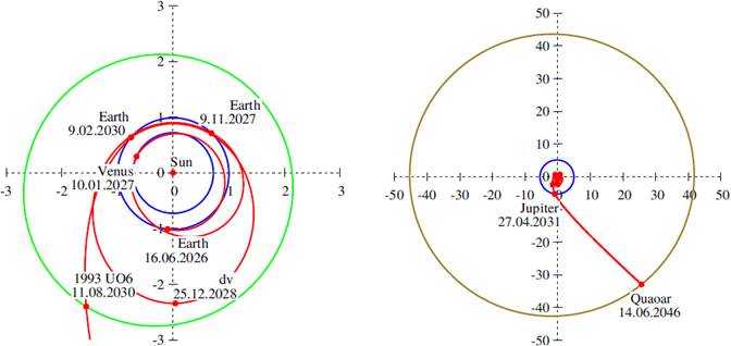
Fig. 15 Optimal transfer trajectory (red) to Quaoar in the ecliptic plane, including the EVEE maneuver, the Jupiter swingby and the (155385) 1993 UO6 asteroid encounter. The orbits of the planets are marked in blue, the orbits of the asteroids in green, and the orbit of Quaoar in olive. The departure from the Earth is shown on the left and the whole trajectory on the right. The distances are given in astronomical units. The total time of flight is constrained to 20 years. The color figure can be viewed online. 

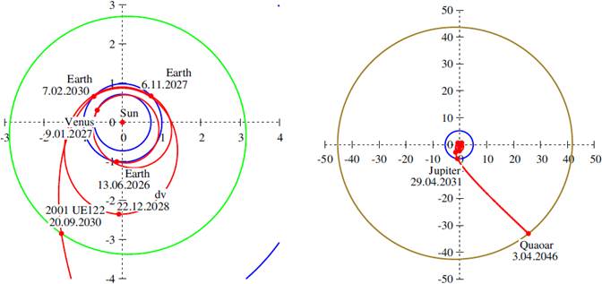
Fig. 16 Transfer type E3. The same as Figure 15, but including the (64378) 2001 UE122 asteroid encounter. The color figure can be viewed online. 

3.4. Summary of the transfers

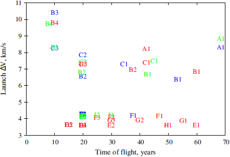
The summary of all optimal transfers shown in this paper is presented here. Figure 17 shows the total ΔV as a function of the time of flight for all transfers. The transfers are represented by their type, with the red ones for transfers to Haumea, blue ones for Makemake, and green ones for Quaoar. Figure 18 shows the ΔV of launch for all trajectories, with the same color code as used in Figure 17.

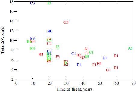
Fig. 17 Total ΔV for all types of optimal transfers as a function of the time of flight. Red: optimal transfers to Haumea; blue: optimal transfers to Makemake; green: optimal transfers to Quaoar. The color figure can be viewed online. 

Fig. 18 ΔV at launch for all types of optimal transfers as a function of the time of flight. Red: optimal transfers to Haumea; blue: optimal transfers to Makemake; green: optimal transfers to Quaoar. The color figure can be viewed online. 

4. Conclusions

The present paper gives results of an analysis of the spacecraft trajectories from the Earth to three of the most interesting Kuiper Belt Objects: Haumea, Makemake, and Quaoar. The trajectories were obtained using different planets to make one or more intermediate swingby(s). The criterion to choose the best trajectories is the minimization of the total ΔV, which does not include the ΔV of the capture maneuver. The 2023-2034 interval is used as a base-line for the launch times for the mission. The results identify trajectories using a total ΔV below 10 km/s with times of flight below 20 years for all the three bodies considered as targets of the mission. Using a multigravity assist maneuver with the Jupiter swingby, one trajectory to each of the bodies is found with a ΔV under 10 km/s and a time of flight below 10 years. Those opportunities are not often repeated, and should be taken into account in the future plans of deep space missions. Considering the less expensive and longer transfers with a duration of 20 years, the possibility of visiting some asteroids of the main belt during the flight is shown, which increases the scientific return of the mission. Those extra observations can be made with only a small increase in the fuel consumed, sometimes below 0.1 km/s.

The authors wish to express their appreciation for the support provided by grants #406841/2016-0 and 301338/2016-7 from the National Council for Scientific and Technological Development (CNPq); Grants #2016/24561-0, 2014/22295-5, 2015/19880-6 and 2016/14665-2 from São Paulo Research Foundation (FAPESP) and for the financial support from the Coordination for the Improvement of Higher Education Personnel (CAPES).