


 nueva página del texto (beta)
 Inglés (pdf)
 Artículo en XML
 Referencias del artículo
 Enviar artículo por email
 Citado por SciELO
  Similares en
SciELO
Similares en
SciELO 
 Permalink
1. Introduction
Radio astronomy has long proven to be an important window into the study of stellar astrophysics, and stellar outflows have been no exception (e.g., Dulk 1995; Güdel 2002; Kurt et al. 2002). For stellar winds a key driver has been the prospect of measuring wind mass-loss rates,
One of the main results from a consideration of free-free excesses formed in the wind is that the spectral energy distribution (SED) at long wavelengths will have a power-law slope with flux
Of greater relevance in recent decades has been the abundance of evidence for clumping in massive star winds. In this regard the literature is voluminous, and there has even been a conference to focus on the topic (Hamann, Feldmeier, & Oskinova 2008). The line-driven winds of massive stars (Castor, Abbot, & Klein 1975; Friend & Abbott 1986; Pauldrach, Puls, & Kudritzski 1986) are known to be subject to an instability (e.g., Lucy & White 1980; Owocki, Castor, & Rybicki 1988). This instability produces shocks in the flow and is a natural culprit for stochastic wind clumping. The clumping is well-known to affect the long wavelength emission because of the density-square dependence of the free-free emissivity. In the presence of clumping, the radio emission is overly bright for a given value of
Clumping affects any density-square emissivity, including recombination lines. Clumping has been incorporated into several detailed complex numerical codes for modeling massive star atmospheres and their winds, such as CMFGEN (Hillier & Miller 1999) and PoWR (Hamann, Gräfener, & Liermann 2006). An important distinction for clumping is between “macroclumping” and “microclumping”. The former leads to modifications of observables that can depend on the shape of the clump and is sometimes synonymous with a “porosity” treatment. The latter occurs when clumps are all optically thin, so that the radiative transfer does not depend on details of clump morphology. Consequently, microclumping can be handled in terms of a scale parameter, and in fact does not alter the SED slope relative to an unclumped wind (Nugis, Crowther, & Willis 1998). Ignace (2016a) considered the impact of macroclumping vs microclumping for ionized winds at long wavelengths.
This contribution is concerned with modeling a radio recombination line (RRL) profile shape that also includes continuum free-free opacity. The problem has been addressed many times before. Rodríguez (1982) derived the line profile shape for this case, with the interest of supplementing the use of the continuum to obtain M with line broadening formed in the same spatial locale to obtain the wind terminal speed
2. Radio recombination line modeling
Various authors have addressed the relevance of non-LTE effects for interpreting observed RRLs. A discussion of progress on the topic can be found in Gordon & Sorochenko (2002). Relevant to wind-broadened emission lines, Viner et al. undertook a calculation of departure coefficients for studies of H II regions. As previously noted, they allowed for spherical outflow and found that line shapes can be asymmetric. Peters, Longmore, & Dullemond (2012) conducted a similar study for H II regions, and elaborated further on line asymmetry for an outflow. However, neither Viner et al. nor Peters et al. explored the possibility of analytic solutions for the radiative transfer. Here, the approach largely follows Ignace (2009), but relaxing the assumption that the line and continuum source functions are equal. The primary assumptions of the model are as follows:
The wind is spherically symmetric in time average.
The wind is optically thick to free-free opacity. The line can be thin or thick.
While the line and continuum source functions may not be equal, they are taken as constant with radius.
Microclumping is included in the treatment, specifically as a power-law distribution1 with radius. Clumping in massive star winds is both predicted and measured to vary with radius (e.g., Runacres & Owocki 2002; Blomme et al. 2002, 2003; Puls et al. 2006).
2.1. Wind Parameters
Spherical symmetry requires the wind to have a strictly radial wind velocity and density. Being optically thick to free-free opacity, only the large radius flow at constant expansion will be considered. The wind terminal speed is represented by
Microclumping is represented as
where
For emissivity
For this study the clumping factor is allowed to vary with radius as a power law, with
The case of m = 0 is for clumping that is constant throughout the flow; m > 0 implies that clumping declines with radius; m < 0 is the opposite case. (Note that some care must be taken with use of the power law for clumping, since D c ≥ 1.)
2.2. Line and Continuum Opacities
The free-free opacity,
where
In the preceding equation, h is Planck’s constant, k is the Boltzmann constant, T C is the temperature of the gas appropriate for the continuum emission, Z i is the root mean square ion charge, ν is the frequency, and g ν is the Gaunt factor.
Figure 1 shows the geometry for evaluating the optical depth τ along a ray. Cylindrical coordinates for the observer are (p, α, z), with the observer located at great distance along the +z-axis. Spherical observer coordinates are (r,
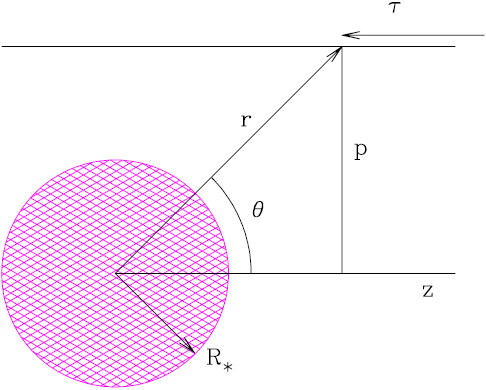
Fig. 1 Coordinate definitions used in the derivation for the line and continuum emission from a spherical ionized wind. See text for explanation. The color figure can be viewed online.
where
At long wavelengths that are the focus of this paper,
The line opacity is somewhat similar to that of the continuum in the sense that there is a dependence on the square of the density for recombination. Assuming that the wind speed is highly supersonic, the line optical depth can be approximated from Sobolev theory (Sobolev 1960). The line optical depth becomes
where
For the case of constant expansion of the wind at
Also note that
where the power-law dependence of D
cl with radius has been substituted into the expression, along with
2.3. Solution for the Case of S L = S C
When the line and continuum source functions are the same, let
where
When the wind is optically thick, such that the excess emission from the wind greatly exceeds the attentuated stellar emisison through the wind, the radiative transfer has a well-known solution when there is no clumping (Panagia & Felli 1975; Wright & Barlow 1975). When constant clumping is present
Ignace (2009) also showed that an analytic solution can result with a power-law distribution in the clumping. The following integral relation will be found of general use in subsequent steps:
where
For the case at hand, the continuum optical depth is
where the second line above uses a change of variable to
The flux of continuum emission becomes
In the Rayleigh-Jeans limit, the continuum flux will have a power-law slope of
Within the line, the solution is really no more complicated. Again, Ignace (2009) showed that
While the argument of the exponential now has two terms, the form of the integral is just like that of the pure continuum. The analytic result is
Note that
2.4. Solution for the Case of SL ≠ SC
In the previous section, a relatively complicated radiative transfer problem for line and continuum was found to have an analytic solution. The simplifications required to obtain that solution were spherical symmetry, time-independent flow, and the limit of constant wind expansion. Variation in the clumping factor could be included if the variation could be treated as a power law. Especially important was that both the free-free and line opacities scaled as the square of density.
The final key assumption was that the line and continuum source functions were equal. However, this assumption can be relaxed to allow for unequal source functions (yet still constant throughout the flow at large radius). In this case the solution for the emergent intensity is more complicated, and becomes
This expression has three terms. A ray at impact parameter
When
For this expression the first term closely mimics the result from the preceding section when
The flux still has an analytic solution. However, an additional standard integral relation is required, of the form
This relation can be applied to the solution for the flux by allowing
The flux in the continuum, outside the velocities of the line, is the same as in the preceding section. However, within the line, the flux now becomes
where
and
It is frequently the case that line profile data are plotted as continuum normalized. The continuum-normalized emission line profile is given by
where
and
where the negative anticipates that the Gamma function in the numerator is also negative.
Note the following special cases. Of course, where there is no line opacity, the radio SED will be a power law in wavelength with
for SC = Bν (TC ). The opposite extreme occurs when the line opacity is significant, but the continuum is negligible. The emission line profile shape becomes
Note that the line shape is symmetric about line center in the limit of a strong line. Wavelength dependence pertinent to the specific line transition is implied through the factors SL and TL.
Equation (27) is the main result of this
study. The first term represents a symmetric component to the emission line
profile. The subsequent two terms contribute generally to asymmetric influences
to the line in the form of G
m(θ). These influences depend on the clumping power-law exponent
m, on the ratio of the source functions S
L
/S
C
, and on the ratio of optical depths T
L
/T
C
. Note that if
3. Results
Figures 2-4 provide illustrative results for line profile shapes. Figure 2 shows results for m = −0.5 (i.e., clumping that increases with radius); Figure 3 for m = 0 (i.e., clumping that is constant with radius); and Figure 4 for m = +1 (i.e., clumping that declines with radius). Each figure has 4 panels: upper left is for δ LC = −0.15, lower left is for δ LC = +0.23, upper right is for δ LC = +0.62, and lower right is for δ LC = +1.0 for Figures 2 and 3, but δ LC = −0.1, 0.4, 0.9, and 1.4 for Figure 4. Each panel has 5 line profiles, with tLC = 0.32, 0.56, 1.0, 1.8, and 3.2, from the weakest line to the strongest. The profiles are continuum normalized and plotted against velocity shift, wz. Note that each panel has a different ordinate scale.
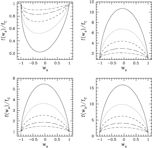
Fig. 2 Continuum normalized emission line profiles for the case of m = −0.5. The 4 panels are: upper left for δLC = −0.15, lower left for δLC = +0.23, upper right for δLC = +0.62, and lower right for δLC = +1.0. In each panel, the 5 line profiles are shown for tLC = 0.32 (dot-dashed), 0.56 (long dashed), 1.0 (short dashed), 1.8 (dotted), and 3.2 (solid), from the weakest line to the strongest. Lines are plotted against normalized velocity shift. Note that each panel has a different scale.
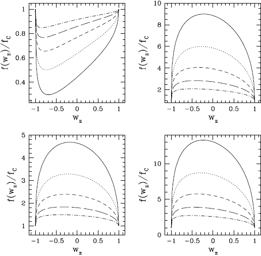
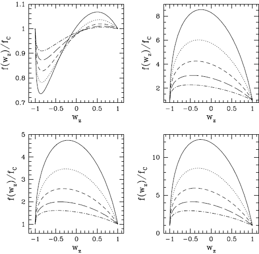
When
For
The line profiles display some degeneracy between δ LC and t LC . As tLC becomes large, asymmetry in the line shape lessens, in the sense that the peak emission shifts closer to line center. A large line optical depth means that a (positive) δ LC has less influence on the line shape. Generally, t LC controls the degree of asymmetry in the line, and δ LC acts as an overall amplitude for the line emission (or line equivalent width).
4. Conclusions
The focus of this contribution has been to high-light the asymmetry of RRLs arising from a spherical wind using an analytic derivation. Previous analytic work produced symmetric line shapes. Numerical calculations have demonstrated that asymmetric lines can be produced. Here, with the assumption of constant but unequal line and continuum source functions, asymmetric line shapes are produced. The derivation allows for the presence of microclumping in the wind in terms of a power-law distribution (rising or declining with radius from the star). While the clumping distribution can impact line asymmetry, the line asymmetry results even with constant clumping, or no clumping whatsoever. Under the model assumptions, emission line asymmetry arises from the continuum opacity (specifically the appearance of the term with G m(θ) in equation 27) that absorbs the redshifted emission from the far hemisphere more than the blueshifted emission from the near hemisphere. The result is a line shape with blueshifted emission peak. (The same effect arises in X-ray lines; c.f., Ignace 2016b).
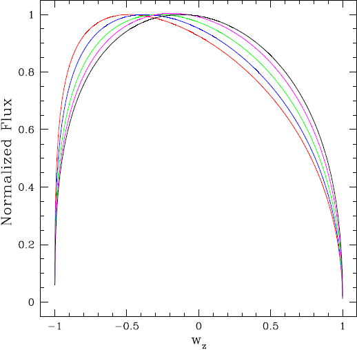
Fig. 5 The line profiles for the case m = 0.0 shown to highlight the evolution of line asymmetry as a function of tLC . The line profiles have been continuum subtracted and normalized to a peak emission of unity. The parame-ter δLC = 0.5 was held fixed. The line profiles are shown for log tLC = −0.5 (red), −0.125 (blue), +0.25 (green), +0.625 (magenta), and +1.0 (black). The color figure can be viewed online.
RRLs are vigorously pursued as a diagnostic of source properties, from kinematics to geometrical aspects. Peters, Longmore, & Dullemond (2012) have made an in-depth study of various factors that affect the flux of line emission and the shape of the line profile, including line asymmetry. Observational motivation for understanding line asymmetry of RRLs includes some objects as the early-type binary MWC349, specifically the H76α line (Escalante et al. 1989). Understanding the line formation is key for distinguishing between radiative transfer effects for the line formation versus the influence of aspherical effects intrinsic to the source, such as binarity, or asymmetric mass-loss, or flow geometry. Applications for such effects include emission-line objects like MWC349 (e.g., LkHα 101; Thum et al. 2013), outflow from star-forming clumps (e.g., Kim et al. 2018), and planetary nebulae (e.g., Ershov & Berulis 1989; Sánchez Contreras et al. 2017). Analytic solutions are valuable to these studies in two main respects: (a) they allow for rapid evaluation of parameter space that can be honed with more detailed numerical calculations to fit the data, and (b) they are important for providing non-trivial benchmarks against which numerical codes can be tested.
The author expresses appreciation to an anony-mous referee for several helpful comments.

