1. Introduction

The Sun has been observed for several decades in many frequencies of the electromagnetic spectrum. The first reported studies of the Sun in the mid infrared range (MIR) were made in the seventies (^{Ohki & Hudson 1975}). Among the results obtained in those years, it can be mentioned that low fluxes were found at the spot areas (^{Hudson 1975}), which locates the origin of this emission in the low atmosphere, near the photosphere. During the following decades no devoted solar instruments were regularly operating at MIR and few observations were reported. The first reported MIR flare was a M7.9 GOES class, observed on March 13, 2012 at 10µ (30 THz) by ^{Kaufman et al. (2013)}, and after that other flares (M2.0 and X2.0) were observed by ^{Kaufmann et al. (2015)}. Recently, ^{Penn et al. (2016)} reported a C7.0 GOES class flare observed at 8.6 and 4.9µm. These flares were simultaneously detected at other wavelengths and it seems that the association between the MIR and white light emission is common.

Until just a few years ago, the flux of solar flares was considered to reach a maximum at microwave frequencies, around 5-10 GHz, and to decrease toward higher frequencies. About a decade ago, flares were seen at 212 and 405 GHz (sub-THz range) noting that the flux grew with frequency (^{Kaufman et al. 2013}). Various mechanisms have been proposed to explain this behavior. It could be due, for instance, to particles different from those responsible of the microwave emission, such as relativistic positrons generating synchrotron emission. However, the origin of this new spectral component of the solar flare emission is still under debate (^{Fleishman & Kontar 2010}). In such flares also MIR has been detected, showing a time evolution similar to that at the sub-THz emission (^{Kaufmann et al. 2015}).

The few MIR flares above described are the only ones reported. The MIR emission is considered to be of thermal origin. However, the similarity of the MIR time profiles with sub-THz profiles and other wavelength profiles (such as hard X-ray) indicates possible non-thermal emission.

Even though there are few observations at the MIR and sub-THz ranges, they provided interesting information about flares and showed that they are more complex than thought a few years ago. These frequence ranges can still give results for a better understanding of the solar activity, and of the Sun in general. To gain better insight into the emission mechanisms involved in the flare phenomena, requires more observations, in particular at the MIR wavelength range.

Astronomical observations at MIR wavelengths are limited by the high opacity of the Earth’s atmosphere. In addition, the opacity is highly variable over several time-scales. In the observations, opacity fluctuations lead to variations that overplot the solar emission. As a result, flares and flux fluctuations of solar origin are more difficult to distinguish. Nevertheless, during winter, the opacity at high altitudes in central Mexico is low, and quite stable for time intervals longer than one hour (^{Pérez-León 2013}). Solar flares last from a few minutes to about an hour. Therefore, at these sites, it is feasible to obtain more stable observations and to detect flares and, possibly, solar flux variations.

2. Characteristics of the mir telescope

We performed simulations of various telescope optical layouts with mirrors and lenses and analized the spot diagrams obtained. In some layouts with parabolic mirrors, the spots lie inside the Airy disk, so that the spatial resolution is determined by the diffraction limit; however, they produce a coma distortion. Hyperbolic surfaces have a better performance. Hence, we selected a Ritchey-Chretien 6-inch telescope, whose plate scale is about 2.5′′/mm.

Various detectors were also analyzed, among them microbolometers and pyroelectric ones. A Melexis 16×4 pixels non-cooled pyroelectric array detector was used at the focal plane of the telescope (Figure 1). The field of view for the whole detector is of 9.6′ × 2.4′ with a resolution of 36′′/pixel. This means that the field covered by the detector has a length, at the sides of the 16 pixels, of about 1/3 of the solar diameter.

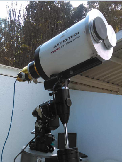
Fig. 1 The Solar Infrared Telescope with the housings for the germanium and Mylar filters at the aperture. The Mylar filter is used for visible light observations. 

Two germanium windows were used, the first with a diameter of 75 mm and a thickness of 5 mm. Mounted in a holder case this window has an apperture of 72 mm diameter. The second germanium window has a diameter of 12.5 mm and a thickness of 1 mm. The transmittance of the first window is 45% between 2µm and 25µm. For the second window, the transmittance is 95% between 8 and 12µm (Thorlabs, Inc., 2017, www.thorlabs.com). The surface of both sides of the first window is natural germanium. The second window has an anti-reflective coating on both sides to improve its transmission in the MIR. The combined transmittance of the two windows, operating in cascade, is about 42% for the spectral range from 8 to 12µm.

The control for the detector was developed using the Cypress PSoC (Programmable System-on-Chip) electronic interface board. The user interface software was written aiming to have an overall view of the observational information, such as time coordinates, detector data and images, in a single computer interface. The values given at the output of the electronics, displayed in the interface and recorded in the data files, are referred to as counts.

The control system of the telescope was developed based on the mounting control made by the Orion company. Various observational regimes were developed in the control software. They include, a scanning of the Sun at different NS and EW disk locations, a tracking of a given region of the Sun, and sky scans.

The mechanical supports for the filters and for the electronics of the detector have been constructed so that the detector and part of its electronics can be located inside an ocular tube near the focal plane of the telescope.

3. Calibrations

Measurements of the response of the detector pixels to a laboratory black-body were made. The counts given by each pixel of the detector for four black body temperatures were measured at the laboratory. For a given temperature, the black-body was scanned, in X-Y directions, by the detector, and the measurementes were recorded. The maximum amplitude for each pixel was identified. This was done at the four temperatures of the black body.

For the 64 pixels of the detector the maximum amplitudes follow a linear relation with the black-body temperature (Figure 2). The maximum amplitudes recorded for each pixel allow us to know the detector flat-field response at each temperature.

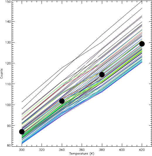
Fig. 2 The color lines represent counts versus temperature of the laboratory black-body for the 64 pixels of the detector. The circles are the 64 values averaged for each temperature. The color figure can be viewed online. 

The ratiation energy received at intervals of area da, frequency dν, solid angle dΩ, during a time interval dt is given by

where I _ν is the specific radiation intensity and θ is the angle between the normal to da and the direction of the incident radiation.

The laboratory black body was observed in a frequency band Δνbb=1.25×1013 Hz, an integration time τ=1 s, a solid angle Ωbb=6.93×10-2 str, with an area per pixel of the detector Adet=4.0×10-8 m² and with θ=0∘. In terms of these parameters the received energy is

In this case, I_ν is the specific intensity for a given temperature of the laboratory black body at the frequency ν . The counts obtained for the four laboratory black-body temperatures (300, 340, 380 and 420 K) are plotted in Figure 2. The averaged values, for each temperature are represented with circles.

The specific intensity is estimated for each black-body temperature using the Planck equation. Then, the energy is computed using equation 2 and the parameters of the laboratory black body observations, given above. The resulting energies are: 1.14 × 10⁻⁷, 2.03 × 10⁻⁷, 3.19 × 10⁻⁷ and 4.62 × 10⁻⁷ J. A two degree polynomial fitted to these energies and the corresponding average value in counts (for each temperature) results in

where C is an observed value in counts, and E the corresponding energy in Joules.

For the center of the quiet Sun a value of 130.5 counts was recorded. The corresponding energy, computed with the fitted polynomial (equation 3), is Es=4.79×10-7 J. To estimate the specific intensity that corresponds to this energy, we now use the parameters for the Sun observations, which are the aperture during the observations Aap=4.07×10-3 m², the solid angle covered by a detector pixel at the telescope focal plane Ωs =2.39×10-8 str, the frequency band Δνs=1.25×1013 Hz, and the time integration τ=1 s. These values are substituted in equation 2, but now for E_s. The resulting specific intensity, considering an attenutation of 0.42 by the two germanium windows, is 1.143 ×10-9 J Hz-1s-1m-2str-1, which corresponds, according to the black-body Planck equation, to a temperature of 4825 K. Since the field of view of a detector pixel pointing to the disk center is fully covered, then this corresponds to the brightness temperature. This value is similar to the numbers reported in other works for similar wavelengths. For example, ^{Shimabukuro & Stacey (1968)} give 5036 K at 11.1µm and 5160 K at 8.63µm. From these values, one may expect a brightness temperature of about 5100 at 10µm. However, ^{Trottet et al. (2015)} applied a model of the quiet Sun to estimate the brightness temperature, obtaining 4700 K. Also, using two flare atmospheric models, they obtained brightness temperatures of 4900 and 5000 K prior to the beginning of the flare. Our value is similar to those obtained in other works.

4. Observations

Figure 3 shows curves obtained by scanning the solar disk at different EW locations on the Sun. An image obtained by scans like these is shown in Figure 4, where two active regions (AR) are seen, one on the upper-left quadrant and another on the lower-right quadrant of the solar disk. In Figure 5 a solar scan shows the quiet Sun and also the AR seen on the upper-left quadrant of Figure 4. A decrease of the amplitude at the location of this AR is seen. This decrease is about 0.008 of the quiet Sun amplitude. By computing the standard deviation around the disk center, it was found that the signal to noise ratio is ≈ 1000. Then, the sensitivity is of 4.8 K.

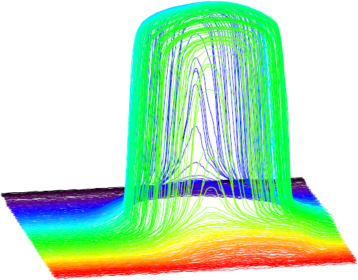
Fig. 3 Scans of the Sun taken with the solar telescope at different X, Y locations across the solar disk. The color figure can be viewed online. 

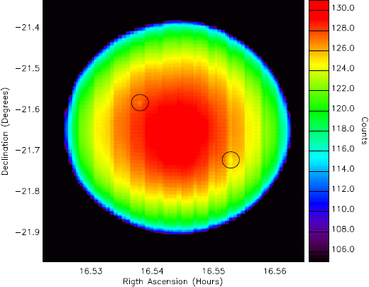
Fig. 4 Image made using the data of scans such as those of Figure 3. Two active regions are seen, one on the upper-left quadrant, denoted by the upper circle, and another active region on the lower-right quadrant of the disk, denoted by the lower circle. The color figure can be viewed online. 

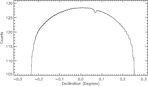
Fig. 5 North-South scan of the Sun across the active region seen on the upper-left quadrant of the disk (Figure 4). 

The ^{Trottet et al. (2015)} estimations of the excess brightness temperature during the maximum of the flare they observed at 10µm are 200 and 300 K, respectively, for the two flare models, which correspond to 0.041 and 0.060 of the quiet Sun brightness temperature. The amplitude we are able to detect, at 1σ, is 0.001 of the quiet Sun. Hence, we could detect a flare as that observed by ^{Trottet et al. (2015)}, and also as that observed by ^{Penn et al. (2016)}, whose maximum amplitudes at 8.6 and 4.9µm, relative to the quiet Sun, are 0.032 and 0.023, respectively.

One of the purposes of developing a portable telescope is to temporarily install it at high altitude sites, where the atmospheric opacity is low, to conduct observation campaigns. Also, to use it in expeditions for solar eclipse observations. We observed the August 21, 2017 solar eclipse. In Figure 6, the time curves obtained for various pixels during the eclipse are shown. It may be seen that the amplitude decreased to a low value, where it remained during the eclipse time, and then again increased to the level previous to the eclipse. Further studies of the solar limb could be done based on solar eclipse data, since the spatial resolution can be improved and complemented with data of scans of the quiet Sun. With the present sensitivity we are able to detect flares, as those above described. It can be better at sites with low atmospheric opacity. We are also developing a camera to estimate the atmospheric opacity at the same wavelength.

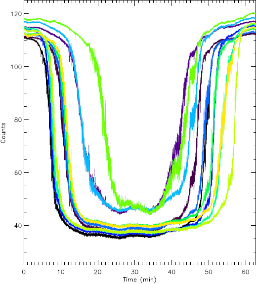
Fig. 6 Time curves of the amplitude recorded at various pixels during the 21 August 2017 eclipse. The time is given in minutes from T_lOC =13:19:55, local time, which is T_lOC =T_UTC -5. It may be seen that at some pixels the amplitude drops to lower values while at others it remains near the level previous to the eclipse. The color figure can be viewed online. 

5. Conclusions

A mid infrared solar telescope centered at 10µm was developed with a 6-inches Ritchey-Cretien optical system by using a 4 × 16 pixels pyroelectric detector at its focal plane. Under the conditions of the preliminary observations here reported, we reached a sensitivity of about ≈1000 of the quiet Sun. The spatial resolution was of 36′′.

We acknowledge the technical team of UNAM at Tonantzintla observatory for their help during two observation campaigns.