2.1. Systematic Effects on the HI and H₂ -to-Stellar Mass Correlations

To reduce potential systematic effects that can bias how we derive the HI and H₂-to-stellar mass correlations we homogenize all the compiled observations to the same basis. Following, we discuss some potential sources of bias/segregation and the calibration that we apply to the observations. It is important to stress that to infer scaling correlations, as those of the gas fraction as a function of stellar mass, it is important to have a statistically representative and unbiased population of galaxies in each mass bin. Thus, there is no need to have mass limited volume-complete samples (see also § 4.1). However, a volume-complete sample assures that possible biases of the measure in question due to selection functions in galaxy type, color, environment, surface brightness, etc., are not introduced. The main expected bias in the gas content at a given stellar mass is due to the galaxy type/color; this is why we need to separate the samples at least into two broad populations, LTGs and ETGs.

2.2. The Compiled HI Sample

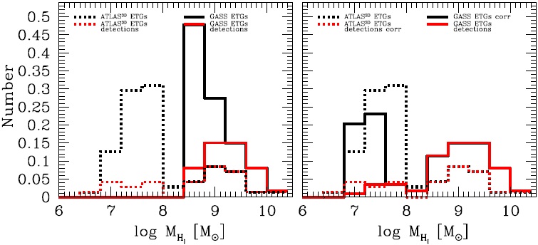
Appendix A presents a summary of the HI samples compiled in this paper (see also Table 2). Table 3 lists the total numbers and fractions of compiled galaxies with detection and non-detection for each galaxy population. Table 4 lists the number of detected and non-detected galaxies for the golden, silver, and bronze categories listed above (§ 2.1.5).

Figure 1 shows the mass ratio R_HI ≡ M_HI /M_∗ vs. M_∗ for the compiled samples. Note that we have applied some corrections to the reported samples (see above) to homogenize all the data. The upper and bottom left panels of Figure 1 show, respectively, the compilations for LTGs and ETGs. The different symbols indicate the source reference of the data and the downward arrows are the corresponding upper limits of the HI-flux for non-detections. We also reproduce the mean and standard deviation of different mass bins as reported in ^{Maddox et al. (2015)} for a cross-match of the ALFALFA and SDSS surveys. As mentioned in the Introduction, the ALFALFA survey is biased to high R_HI values, specially towards the low mass side. Note that the small ALFALFA subsample of dwarf galaxies by ^{Huang et al. (2012b, dark purple dots)} was selected mainly as an attempt to take into account low-HI mass galaxies at the low-mass end.

Fig. 1 Atomic gas-to-stellar mass ratio as a function of M_∗. Upper panels: Compiled and homogenized data with information on R_HI and M_∗ for LTGs (the different sources are indicated inside the left panel; see Appendix A for the acronyms and authors); downward arrows show the reported upper limits for non-detections. The blue triangles with thin error bars are mean values and standard deviations from the v.40 ALFALFA and SDSS crossmatch according to ^{Maddox et al. (2015)}; the ALFALFA galaxies are biased toward high values of R_HI (see text). Right panel is the same as left one, but with the data separated into three categories: Golden, Silver, and Bronze (yellow, gray, and brown symbols, respectively). The red and blue lines are Buckley-James linear regressions (taking into account non-detections) for the high- and low-mass regions, respectively; the dotted lines show extrapolations from these fits. Squares with error bars represent the mean and standard deviation of the data in different mass bins, taking into account non-detections by means of the Kaplan-Meier estimator. Open circles with error bars show the corresponding median and 25-75 percentiles. Estimates of the observational uncertainties are shown in the panel corners (see text). Lower panels: Same as upper panels but for ETGs. In the right panel, we have corrected for distance the galaxies with upper limits from GASS to make them consistent with the distances of the ATLAS3D sample (see text); the upper limits from the latter were increased by a factor of two to homogenize them to the ALFALFA instrument and signal-to-noise criteria. For the bins where more than 50% of the data are upper limits, the median and percentiles are not calculated. The color figure can be viewed online. 

2.3. The Compiled H₂ Sample

Since the emission of cold H₂ in the ISM is extremely weak, a tracer of the H₂ abundance should be used. The best tracer from the observational point of view is the CO molecule due to its relatively high abundance and its low excitation energy. The H₂ mass is related to the CO luminosity through a CO-to-H₂ conversion factor: MH2 = α_CO L_CO. This factor has been determined in molecular clouds in the Milky Way (MW), αCO,MW = 3.2 (K km s⁻¹ pc⁻¹)⁻¹, with a systematic uncertainty of 30%. It was common to assume that this conversion factor was the same for all galaxies. However, several pieces of evidence show that αCO is not constant, and that it depends mainly on the gas-phase metallicity, increasing as the galaxy metallicity decreases (e.g., ^{Boselli et al. 2002}; ^{Schruba et al. 2012}; ^{Narayanan et al. 2012}; ^{Bolatto et al. 2013}, and references therein). At firstorder, αCO changes slowly for metallicities larger than 12 + log₁₀(O/H) ≈ 8.4 (approximately half the solar one) and increases considerably as the metallicity decreases. Here, we combine the dependence of αCO on metallicity given by ^{Wolfire et al. (2010)} and the observed mass-metallicity relation to obtain an approximate estimation of the dependence of αCO on M_∗ for LTGs; see Appendix C for details. We are aware that the uncertainties involved in any metallicity-dependent correction remain substantial (Bolatto et al. 2013). Note, however, that our aim is to introduce and explore at a statistical level a reasonable mass-dependent correction to the CO-to-H₂ factor, which must be better than ignoring it. In any case, we present results both for α_CO = α_CO,MW and our inferred mass-dependent α_CO factor. In fact, the mass-dependent factor is important only for LTGs with M_∗ ≲ 3 × 10¹⁰ M_⊙; for larger masses and for all ETGs, α_CO ≈ α_CO,MW¹.

Appendix B presents a description of the CO (H₂) samples that we utilize in this paper. Table 3 lists the number of galaxies with detections and upper limits in the compilation sample in terms of morphology. Table 4 lists the number of detections and upper limits for the golden, silver, and bronze categories mentioned above (§ 2.1.5).

Figure 2 shows the mass ratio RH2≡ MH2 /M_∗ vs. M_∗ for the compiled samples. Similarly to the R_HI vs. M_∗ relation, we applied some corrections to observations in order to homogenize our compiled sample and to allow a more consistent comparison between the different samples. The upper and bottom left panels of Figure 2 show, respectively, the compiled datasets for LTGs and ETGs.

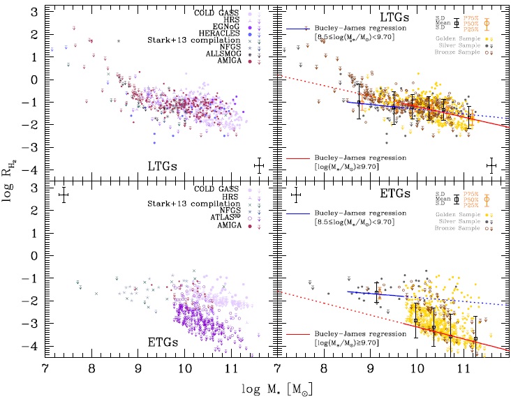
Fig. 2 Molecular gas-to-stellar mass ratio as a function of M_∗. Upper panels: Compiled and homogenized data with information on RH2 and M_∗ for LTGs (see inside the panels for the different sources; see Appendix B for the acronyms and authors); downward arrows show the reported upper limits for non-detections. Right panel is the same, but with the data separated into three categories: Golden, Silver, and Bronze (yellow, gray, and brown symbols, respectively). The red and blue lines are Buckley-James linear regressions (taking into account non-detections). The dotted lines show extrapolations from these fits. The green dashed line shows an estimate for the RH2 -M_∗ relation inferred from combining the empirical SFR MH2 and SFR-M_∗ correlations for blue/star-forming galaxies (see text for details). Squares with error bars are the mean and standard deviation of the data in different mass bins, taking into account non-detections by means of the Kaplan-Meier estimator. Open circles with error bars are the corresponding median and 25-75 percentiles. Estimates of the observational/calculation uncertainties are shown in the panel corners (see text). Lower panels: The same as upper panels but for ETGs. In the right panel, we have corrected for distance the galaxies with upper limits from COLD GASS to make them consistent with the distances of the ATLAS^3D sample (see text). For the bins where more than 50% of the data are upper limits, the median and percentiles are not calculated. The color figure can be viewed online. 

3.1. R_HI vs. M_∗

In Figure 3, results for log R_HI vs. log M_∗ are shown for LTGs (upper panels) and ETGs (lower panels). From left to right, the regressions for samples in the Golden, Silver, and Bronze categories are plotted. The error bars correspond to the 1σ scatter of the regression. Each line covers the mass range of the corresponding sample. The blue/red dashed lines and shaded regions in each panel correspond to the mean and standard deviation values calculated with the Kaplan-Meier estimator in mass bins for all the compiled LTG and ETG samples, previously plotted in Figures 1 and 2, respectively. However, the yellow, gray, and brown dots connected with thin solid lines in each panel are the mean values in each mass bin calculated only for the Golden, Silver, and Bronze samples, respectively. The standard deviations are plotted as dotted lines. In the following, we discuss the results shown in Figure 3.

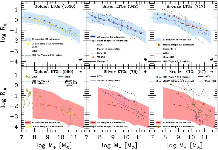
Fig. 3 Atomic gas-to-stellar mass ratio as a function of M_∗ for the Golden, Bronze, and Silver LTGs (upper panels) and ETGs (lower panels). The mean and standard deviation in different mass bins, taking into account upper limits by means of the Kaplan-Meier estimator, are plotted for each case (filled circles connected by a dotted line and dotted lines around, respectively). For comparison, the mean and standard deviation (dashed lines and shaded area) from all the LTG (ETG) samples are reproduced in the corresponding upper (lower) panels. For each sample compiled and homogenized from the literature, the Buckley-James linear regression is applied, taking into account upper limits. The lines show the result, covering the range of the given sample; the error bars show the corresponding standard deviations obtained from the regression. When the data are too scarce and dominated by upper limits, the linear regression is not applied but the data are plotted. The numbers of LTG and ETG objects in each category are indicated in the respective panel. The color figure can be viewed online. 

Golden category: For LTGs, the three samples grouped in this category agree well among themselves in the mass ranges where they overlap; even the 1σ scatter of each sample does not differ significantly⁴. Therefore, as expected, these samples provide unbiased information for determining the R_HI -M_∗ relation of LTGs from log(M_∗/M_⊙ )≈ 7.3 to 11.4. For ETGs, the deviations of the Golden linear regressions among themselves and compared to all galaxies are within the 1σ scatter, which is actually large. If no corrections to the upper limits of the GASS and ATLAS^3D are applied, then the regression for the former would be significantly above the regression for the latter. Within the large scatter, the three Golden samples of ETGs seem not to be particularly biased, and they cover a mass range from log(M_∗/M_⊙)≈ 8.5 to 11.5. At smaller masses, the Updated Nearby Galaxy Catalog (UNGC) sample provides mostly only upper limits to R_HI.

Silver category: The LTG and ETG samples in this category, as expected, show more dispersed distributions in their respective R_HI-M_∗ planes than those from the Golden category. However, the deviations of the Silver linear regressions among themsleves and compared to all the galaxies are within the corresponding 1σ scatter. If any, there is a trend of the Silver samples to have mean R _HI values above the mean values of all galaxies especially for ETGs. Since the samples in this category are volume-complete, (they were specially constructed to study HI gas content), a selection effect towards objects with non-negligible or higher than the mean HI content can be expected. In any case, the biases are small. Thus, we decided to include the Silver samples to infer the R_HI-M_∗ correlations in order to slightly increase the statistics (the number of galaxies in this category is actually much smaller than in the Golden category), specially for ETGs of masses smaller than log(M_∗/M_⊙)≈ 9.7 (see Table 4).

Bronze category and effects of the environment: The very isolated LTGs (from the UNAMKIAS and Analysis of the interstellar Medium of Isolated GAlaxies -AMIGAsamples) have HI contents higher than the mean of all the galaxies, especially at lower masses: log R_HI is 0.1 − 0.2 dex larger than the average at log(M_∗/M_⊙)>∼ 10 and these differences increase up to 0.6 − 0.3 dex for 8 < log(M_∗/M_⊙) < 9, though the number of galaxies at these masses is very small. The HI content of the ^{Bradford et al. (2015)} isolated dwarf galaxies is also larger than the mean of all the galaxies but not by a factor larger than 0.4 dex. For isolated ETGs, the differences can attain an order of magnitude and are at the limit of the upper standard deviations around the means of all the ETGs. Thus, while isolated LTGs have somewhat larger R_HI ratios on average than galaxies in other environments, in the case of isolated ETGs, this difference is very large; isolated ETGs can be almost as gas rich as LTGs. In the Bronze group we have included also galaxies from the central regions of the Virgo Cluster, as reported in HRS and ATLAS^3D (only ETGs for the latter). According to Figure 3, the LTGs in this high-density environment are clearly HI deficient with respect to LTGs in less dense environments. For ETGs, the HI content is very low but only slightly lower on average than the HI content of all ETGs. It should be noted that ETGs, in particular the massive ones, tend to be located in high-density environments.

We conclude that the HI content of galaxies is affected by the effects of extreme environments. The most remarkable effect occurs for ETGs, which in a very isolated environment can be as rich in HI as LTGs. Therefore, we decided not to include galaxies from the Bronze category to determine the R_HI-M_∗ correlation of ETGs. In fact, our compilation in the Golden and Silver categories includes galaxies from a range of environments (for instance, in the largest compiled catalog, UNGC, 58% of the galaxies are members of groups and 42% are field galaxies, see ^{Karachentsev et al. 2014}) in such a way that the R_HI-M_∗ correlation determined below should represent an average of different environments. Excluding the Bronze category for the ETG population, we avoid biases due to effects of the most extreme environments. For LTGs, the inclusion of the Bronze category does not introduce significant biases in the R_HI-M_∗ correlation of all galaxies but it helps to improve the statistics. The mean values of R _HI in mass bins above ≈ 10⁹ M_⊙ are actually close to the mean values of the entire sample (compare the brown solid and blue dashed lines); at smaller masses the deviation increases, but the differences are well within the 1σ dispersion.

3.2. RH2 vs. M_∗

In Figure 4, we present plots similar to Figure 3 but for log RH2 vs. log M_∗. The symbol and line codes are the same in both figures. In the following, we discuss the results shown in Figure 4.

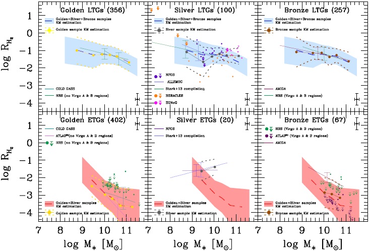
Fig. 4 Same as Figure 3 but for the molecular gas-to-stellar mass ratio. The color figure can be viewed online. 

Golden category: For LTGs, the two samples grouped in this category agree well among themsleves and with the overall sample, though for masses < 10¹⁰ M_⊙, where the Golden galaxies are only those from the HRS sample, the average RH2 values are slightly larger than those from the overall LTG sample (compare the solid yellow and dashed blue lines), but still well within the 1σ scatter (shaded area). For ETGs, the deviations of the linear regressions of the Golden samples among themselves, and compared to all ETGs, are within the respective 1σ scatters, which are actually large. If no corrections to the upper limits of the GASS and ATLAS^3D were applied, then the regression for the former would be significantly above the regression for the latter. Summarizing, the Golden samples of LTGs and ETGs do not show particular shifts in their respective RH2 - M_∗ correlations. Therefore, the combination of them is expected to provide reliable information for determining the respective RH2 - M_∗ correlations: for LTGs in the ≈ 10^8.5 − 10^11.5 M_⊙ mass range, and for ETGs, only for M_∗ ≳ 10¹⁰ M_⊙.

Silver category: The LTG samples present a dispersed distribution in the log RH2 -logM_∗ plane but well within the 1σ scatter of the overall sample (shaded area). The mean values in mass bins from samples of the Silver category are in reasonable agreement with the mean values from all the samples (compare the gray solid and blue dashed lines). Therefore, the Silver samples, though scattered and not complete in any sense, seem not to exhibit a clear systematical shift in their H₂ content. We include these samples to infer the RH2 - M_∗ correlation of LTGs. For ETGs, the two Silver samples provide information for masses below M_∗ ≈ 10¹⁰ M_⊙, and both are consistent with each other. Therefore, we include these samples to infer the ETG RH2 -M_∗ correlation down to M_∗ ≈ 10^8.5 M_⊙.

Bronze category and the effects of environment: The isolated (from the AMIGA sample) and Virgo central (from the HRS catalog) LTGs have H₂ contents similar to the mean in different mass bins of all the galaxies. If any, the Virgo LTGs have on average slightly higher values of RH2 than the isolated LTGs, especially at masses smaller than M_∗ ≈ 10¹⁰ M_⊙. Given that LTGs in extreme environments do not segregate from the average RH2 values at different masses of all galaxies, we include them for calculating the RH2 -M_∗ correlation of LTGs. For ETGs, the AMIGA isolated galaxies have on average values of RH2 significantly higher than the mean of other galaxies, while those ETGs from the Virgo central regions (from HRS and ATLAS^3D; mostly upper limits), seem to be on average consistent with the mean of all the galaxies, though the scatter is large. Given the strong deviation of isolated ETGs from the mean trend, we prefer to exclude galaxies from the Bronze category to determine the ETG RH2 -M_∗ correlation. We conclude that the H₂ content of LTGs is weakly dependent on the environment of galaxies, but in the case of ETGs, very isolated galaxies have systematically higher R_H2 values than galaxies in more dense environments.

4.1. Strategy for Constraining the Correlations

In spite of the diversity in the compiled samples and their different selection functions, the exploration presented in the previous section shows that the HI and H₂ contents as a function of M_∗ for most of the samples compiled here do not segregate significantly among them. The exception are the Bronze samples for ETGs. Therefore, the Bronze ETGs are excluded from our analysis. The strong segregation is actually by morphology (or color, or star formation rate), and this is why we have separated from the beginning the compiled data into two broad galaxy groups, LTGs and ETGs.

To determine gas-to-stellar mass ratios as a function of M_∗ we need (1) to take into account the upper limits of undetected galaxies in radio, and (2) to evaluate the correlation independently of the number of data points in each mass bin. If we have many data points in some mass bins and only a few ones in other mass bins (as would happen if we use, for instance, a mass-limited volume-complete sample, with many more data points at smaller masses than at larger masses), then the overall correlation of R_HI or RH2 with M_∗ would be dominated by the former, probably giving incorrect values of R_HI or RH2 at other masses. In view of these two requirements, our strategy to determine the logR _HI-logM_∗ and log RH2 -logM_∗ correlations is as follows:

4.2. The HI-to-Stellar Mass Correlations

In the upper left panel of Figure 5, along with the data from the Golden, Silver, and Bronze LTG samples, the mean and standard deviation (squares and black error bars) calculated for each mass bin with the Kaplan-Meier method are plotted. In the lower left panel, the same is plotted but for the Golden and Silver ETG samples (recall that the Bronze samples are excluded in this case). We see that the total standard deviations in log R_HI, σ_dat, do not evidence a systematical dependence on mass both for LTGs and ETGs. Then, we can use a constant value for each case. For LTGs, the standard deviations have values around 0.45-0.65 dex with an average of σ_dat ≈ 0.53 dex. For ETGs, the standard deviations are much larger and more dispersed than for LTGs (see § 4.4 below for a discussion on why this could be). We assume an average value of σ_dat = 1 dex for ETGs.

Fig. 5 Left panels: The R_HI-M_∗ correlation for LTGs (upper panel) and ETGs (lower panel). Dots are detections and arrows are upper limits for non-detections (for ETGs the Bronze sample was excluded). The squares and error bars show the mean and standard deviation in different mass bins calculated by means of the Kaplan-Meier estimator for censored and uncensored data. The thin error bars correspond to our estimate of the intrinsic scatter after taking into account the observational errors (shown in the panel corners). The solid and long-dashed lines in each panel are respectively the best double- and single-power law fits. The shaded areas show the intrinsic scatter; to avoid overcrowding, for the single power-law fit, the intrinsic scatter is plotted only at one point. The dotted lines are extrapolations of the correlations to low masses, where the data are scarce and dominated by upper limits. Middle panels: Same as in the left panels but for RH2. For the ETG population, the double power-law fit was performed with the conservative constraint that below M_∗ = 10⁹ M_⊙, the low-mass slope is zero. Right panels: The R_gas-M_∗ correlations for LTGs and ETGs as calculated from combining the respective double- and single-power law R_HI-M_∗ and RH2 -M_∗ correlations and taking into account helium and metals (see text). The shaded area and error bar are the (1σ) intrinsic scatter obtained by error propagation of the intrinsic scatter around the corresponding R _HI-M _∗ and RH2 -M_∗ relations. For completeness, the data from our compilation that have determinations of both HI and H₂ masses are also plotted (the obtained correlations are not fits to these data). Dotted lines are extrapolations of the inferred relations to smaller masses. The short dashed lines show the best fits using the double power-law function. The color figure can be viewed online. 

The intrinsic standard deviation (scatter) can be estimated as σintr2≈σdat2-σerr2 (this is valid for normal distributions), where σ_err is the mean statistical error in the log R _HI determination due to the observational uncertainties. In Appendix E we present an estimate of this error, σ_err ≈ 0.14 dex. Therefore, σ_intr ≈ 0.52 and 0.99 dex for LTGs and ETGs, respectively. These estimates should be taken only as indicative values given the assumptions and rough approximations involved in their calculations. For example, we will see in § 5 that the distributions of log R _HI (detections and non-detections) in different mass bins tend to deviate from a normal distribution, in particular for ETGs.

Next, we propose that the HI-to-stellar mass relations can be described by the general function:

where y = R_HI, C is the normalization factor, a and b are the low and high-mass slopes of the function and M*tr is the transition mass. This function is continuous and differentiable. If a = b, then equation (1) describes a single power law, or a linear relation in logarithmic scales. In this case, the equation remains as y(M_∗) = C′(M_∗/M_⊙)^−a. For a ≠ b, the function corresponds to a double power law.

We fit the logarithm of function, equation (1), to the mean values of logR_HI as a function of mass (squares in the left panels of Figure 5) with the corresponding (constant) intrinsic standard deviation as estimated above (thin blue/red error bars). For LTGs, the fit is carried out in the range 7.3 ≲ log(M_∗/M_⊙ )≲ 11.2, and for ETGs in the range 8.5 ≲ log(M_∗/M_⊙)≲ 11.5. The Levenberg Marquardt method is used for the fit (^{Press et al. 1996}). First, we perform the fits to the binned LTG and ETG data using a single power law, i.e., we fix a = b. The dashed orange and green lines with an error bar in the left panels of Figure 5 show the results. The fit parameters are given in Table 5. We note that these fits and those of the Buckley-James linear regression for all the data (not binned) in logarithm are very similar.

Then, we fit to the binned data the logarithm of the double power-law function given in equation (1). The corresponding best-fit parameters are presented in Table 6. We note that the fits are almost the same if the total mean standard deviation, σ_dat, is used instead of the intrinsic one. The reduced χred2 are 0.01 and 0.03, respectively. The fits are actually performed to a low number of points (the number of mass bins) with large error bars; this is why the χred2 are smaller than 1. Note, however, that the error bars are not related to measurement uncertainties but correspond to the population scatter of the data. Therefore, in this case χred2 < 1 implies that while the best fit is good, other fits could be also good within the scatter of the correlations. In the case of the single power-law fits, the χred2 are 0.03 and 0.01, respectively for LTG and ETG.

The double power-law R_HI-M_∗ relations and the estimated intrinsic (1σ) scatter for the LTG (ETG) population are plotted in the left upper (lower) panel of Figure 5 with solid lines and shaded areas, respectively. From the fits, we find for LTGs a transition mass M*tr = 1.74 ×10⁹ M_⊙, with R ∝ M_∗ ^−0.21 and M_∗ ^−0.67 at masses much smaller and larger than this, respectively. For ETGs, M*tr = 1×10⁹ M_⊙, and R_HI ∝ M_∗ ^0.0 and M_∗ ^-0.58, at masses much smaller and larger than this, respectively.

Both the double and single power laws describe well the HI-to-stellar mass correlations. However, the former could be more adequate than the latter. In Figure 1 we plot the Buckley-James linear regressions to the R_HI vs. M_∗ data for the low and high mass regions (below and above log(M_∗/M_⊙)≈ 9.7; for ETGs the regression is applied only for masses above 10⁸ M _⊙); the dotted lines show the extrapolation of the fits. The slope at low masses for LTGs, −0.36, is shallower than the one at high masses, −0.55. For ETGs, there is even evidence of a change in the slope sign at low masses. A flattening of the overall (late + early type galaxies) correlation at low masses has been also suggested by ^{Baldry et al. (2008)}, who have used the empirical mass- metallicity relation coupled with a metallicity-to-gas mass fraction relation (which can be derived from a simple chemical evolution model) to obtain a gasto-stellar mass correlation in a large mass range. Another evidence that at low masses the R_HI-M_∗ relation flattens is shown in the work by ^{Maddox et al. (2015)} already mentioned (see also ^{Huang et al. 2012a}). While the sample used by these authors does not allow to infer the R_HI-M_∗ correlation of galaxies due to its bias towards high R _HI values (see above), the upper envelope of this correlation can be actually constrained; the high-R_HI envelope does not suffer from selection limit effects. As seen for the data from ^{Maddox et al. (2015)} reproduced in the left upper panel of our Figure 1, this envelope tends to flatten at M_∗ ≲ 2 × 10⁹ M_⊙,⁵ which suggests (but does not demonstrate) that the mean relation can also exhibit such a flattening. Another piece of evidence in favor of the flattening can be found in ^{Huang et al. (2012b)}, and more recently in ^{Bradford et al. (2015)} for their sample of low-mass galaxies combined with larger mass galaxies from the ALFALFA survey.

4.3. The H₂ -to-Stellar Mass Correlations

In the upper middle panel of Figure 5, along with the data from the Golden, Silver, and Bronze LTG samples, the mean and standard deviation (error bars) calculated in each mass bin with the KaplanMeier method are plotted. In the lower panel, the same is plotted but for the Golden and Silver ETG samples (recall that the Bronze samples are excluded in this case). The poor observational information at stellar masses smaller than ≈ 5 × 10⁸ M_⊙ does not allow us to constrain the correlations at these masses, both for LTG and ETGs. Regarding the total standard deviations, for both LTGs and ETGs, they vary from mass bin to mass bin but without a clear trend. Then we can use a constant value for both cases. For LTGs, the total standard deviations have values around 0.5-0.8 dex with an average of σ_dat ≈ 0.58 dex. For ETGs, the average value is roughly 0.8 dex. As in the case of HI (previous subsection), we further estimate indicative values for the intrinsic population standard deviations (scatter). For this, we present in Appendix E an estimate of the the mean observational error of the log RH2 determination, σ_err ≈ 0.34 dex. Therefore, the estimated mean intrinsic scatters in log RH2 are σ_intr ≈ 0.47 and 0.72 dex for LTGs and ETGs, respectively. Given the assumptions and approximations involved in these estimates, they should be taken with caution. For example, we will see in § 5 that the distributions of log RH2 (detections and non-detections) in different mass bins tend to deviate from a normal distribution, in particular for the ETGs.

We fit the logarithm of function equation (1), y = RH2, to the mean values of log RH2 as a function of mass (squares in the left panels of Figure 5) with their corresponding scatter as estimated above (thin blue/red error bars), assumed to be the individual standard deviations for the fit. Again, the Levenberg-Marquardt method is used to perform the fit. The fits extend only down to M_∗ ≈ 5 × 10⁸ M_⊙. First, the fits are performed for a singe power law, i.e., we fix a = b. The dashed orange and green lines in the middle panels of Figure 5 show the results. The parameters of the fit and their standard deviations are given in Table 5. The fits are very similar to those obtained using the Buckley-James linear regression to all (not binned) logarithmic data.

Then, we fit the binned LTG and ETG data to the double power-law function equation (1). In the case of the ETG population, we impose an extra condition to the fit: that the slope of the relation at masses below ≈ 10⁹ M_⊙ be flat. The few data at these masses clearly show that RH2 does not increase for smaller M_∗; it is likely that it even decreases, so that our assumption of a flat slope is conservative. The corresponding best-fit parameters are presented in Table 6. As in the case of the R_HI −M_∗ correlations, the reduced χred2 are smaller than 1 (0.04 and 0.10, respectively), which implies that while the best fits are good, other fits could describe reasonably well the scattered data. In the case of the single power-law fits, χred2 were 0.04 and 0.07, respectively for LTG and ETG. The double power-law RH2 -M_∗ relations and their (1σ) intrinsic scatter for the LTG (ETG) population are plotted in the middle upper (lower) panel of Figure 5 with solid lines and shaded areas, respectively. We note that the fits are almost the same if the total mean standard deviation, σ_dat, is used instead of the intrinsic one.

From these fits, we find for LTGs, M*tr = 1.74 × 10⁹ M_⊙, with RH2 ∝ M_∗ ^−0.07 and M_∗ ^−0.47 at much smaller and larger masses than this, respectively. For ETGs, M*tr = 1.02 × 10⁹ M_⊙, with RH2 ∝ M_∗ ^0.00 and M_∗ ^−0.94 at much smaller and larger masses than this, respectively. In the middle upper panel of Figure 5, we plot also the best double power-law fit to the RH2 -M_∗ correlation of LTGs when the αCO factor is assumed constant and equal to the MW value (purple dashed line).

Both the single and double power-law functions describe equally well the RH2 -M_∗ correlations for the LTG and ETG population, but there is some evidence of a change of slope at small masses. In Figure 2, the Buckley-James linear regressions to the RH2 vs. M_∗ data below and above log(M_∗/M_⊙)≈ 9.7 are plotted (in the former case the regressions are applied for masses only above 10⁸ M_⊙); the dotted lines show the extrapolation of the fits. The slopes in the small mass range at low masses for LTGs/ETGs are shallower than those at high masses. Besides, in the case of ETGs, if the single power-law fit shown in Figure 5 is extrapolated to small masses, ETGs of M_∗ ≈ 10⁷ M_⊙ would be dominated in mass by H₂ gas. Red/passive dwarf spheroidals are not expected to contain significant fractions of molecular gas. Recently, ^{Accurso et al. (2017)} have also reported a flattening in the H₂-to-stellar mass correlation at stellar masses below ≈ 10¹⁰ M_⊙.

4.4. The Cold Gas-to-Stellar Mass Correlations

Combining the R_HI-M_∗ and RH2 -M_∗ relations presented above, we can obtain now the R_gas-M_∗ relation, for both the LTG and ETG populations. Here, R_gas = M_gas/M_∗ = 1.4(R_HI + RH2), where M_gas is the galaxy cold gas mass, including helium and metals (the factor 1.4 accounts for these components). The intrinsic scatter around the gas-tostellar mass relation can be estimated by propagating the intrinsic scatter around the HI and H₂ to-stellar mass relations. Under the assumption of null covariance, the logarithmic standard deviation around the logR_gas -logM_∗ relation is given by

The obtained cold gas-to-stellar mass correlations for the LTG and ETG populations are plotted in the right panels of Figure 5. The solid lines and shaded bands (intrinsic scatter given by the error propagation) were obtained from the double powerlaw correlations, while the solid green lines and the error bars were obtained from the single power-law correlations. For completeness, we also plot in Figure 5 those galaxies from our compilation that have determinations for both the HI and H₂ masses. Note that a large fraction of our compilation has no determinations for both quantities at the same time. We fit the results obtained for the single (double) power-law fits, taking into account the intrinsic scatter, to the logarithm of the single (double) power law function given in equation (1) with y = R _gas and report in Table 5 (Table 6) the obtained parameters for both the LTGs and ETGs. The fits for the double power-law are shown as dotted lines in Figure 5. The standard deviations σlog R_gas change slightly with mass; we report an average value for them in Tables 5 and 6. Both for LTGs and ETGs, the mass at which the R_gas-M_∗ correlations change slope is M*tr ≈ 1.7 × 10⁹ M_⊙, the mass that roughly separates dwarf from normal galaxies.

According to Figure 5, the LTG and ETG R_gas- M_∗ correlations are significantly different. The gas content in the former is at all masses larger than in the latter, the difference being maximal at the largest masses. For the LTG population, M_gas ≈ M_∗ on average at log(M_∗/M_⊙) ≈ 9, and at smaller masses, these galaxies are dominated by cold gas; at stellar masses around 2 × 10⁷ M_⊙ , M_gas is on average three times larger than M_∗. For ETGs, there is a hint that at ≈ 10⁹ M_⊙, R_gas changes from increasing as M_∗ is smaller to decreasing at larger masses.

6.1. The Mock Galaxy Mass Functions

6.1.1. Stellar Mass Function

The mock GSMF is plotted in panel (a) of Figure 13 along with the Poisson errors given by the thickness of the gray line; except for the highest masses, the Poisson errors are actually thinner than the line. The mock GSMF is an excellent realization of the empirical GSMF (compare it with Figure 12). We also plot the corresponding contributions to the mock GSMF of the LTG and ETG populations (blue and red dashed lines). As expected, LTGs dominate at small stellar masses and ETGs dominate at large stellar masses. The contribution of both populations is equal (f_early = f_late = 0.5) at M*cross = 10^10.20 M_⊙ (recall that the fraction fearly used here comes from ^{Moffett et al. (2016)}, who included Sa galaxies as ETGs; if consider Sa galaxies as LTGs, then M*cross would likely be higher). In order to predict accurate gas and baryonic mass functions, the present analysis will be further refined in Rodriguez-Puebla et al. (in prep.), where several sources of systematic uncertainty in the GSMF measurement and in the definition of the LTG/ETG fractions will be taken into account. Our aim here is only to test whether the empirical correlations derived in § 4 are roughly consistent with the total HI and H₂ empirical mass functions.

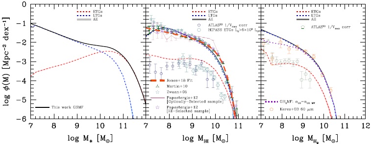
Fig. 13 Panel (a): Total GSMF from the mock catalog that reproduces the empirical GSMF of Figure 12 (solid line). The gray shadow represents the Poisson errors (except for large masses, these errors are thinner than the line thickness). The GSMF from the mock catalog samples very well the empirical GSMF used as input. The blue/red dotted lines and shadows correspond to the LTG/ETG mass function components, using the empirical ETG fraction as a function of M_∗ shown in Figure 12. Panel (b): Same as Panel (a) but for atomic gas, using the mean R _HI-M_∗ relation and its scatter distribution as given in § 5. Several observational GHIMF’s from blind HI samples, and the ETG GHIMF from ATLAS^3D and HIPASS surveys are reproduced (see labels inside the panel). Panel (c): Same as Panel (a) but for molecular gas. The GH₂MF calculated from the ^{Keres et al. (2003)} L_CO function is reproduced. The dotted purple line is the total GH2MF from the mock catalog using a RH2 -M_∗ correlation obtained from our compilation, but assuming that α_CO=α_CO,MW=const., as done in ^{Keres et al. (2003)}. The color figure can be viewed online. 

7.1. The H₂ -to-HI Mass Ratio

The global H₂-to-HI mass ratio of a galaxy characterizes its global efficiency of converting atomic into molecular hydrogen. This efficiency is tightly related to the efficiency of large-scale SF in the galaxy (see e.g., ^{Leroy et al. 2008}). From the empirical correlations inferred in § 4, we can calculate MH2 /M _HI as a function of M_∗ for both the LTG and ETG populations. We do this by using our double power-law fits to the data. The left panel of Figure 14 presents the obtained MH2 /M_HI -M_∗ relations and their 1σ H2 HI scatter calculated by propagating the dispersions in the assumption of null covariance. In this sense, the plotted scatters are upper limits, since there is evidence of some (weak) correlation between the HI and H2 content of galaxies, in particular among those deficient in HI and H₂ (^{Boselli et al. 2014c}). We can plot the same correlations for the mock catalog presented in § 6, which samples the observed GSMF, the LTG and ETG fractions as a function of M_∗, and the empirical correlations inferred by us. The middle panels of Figure 14 present our measures from the mock catalog for LTG (blue), ETG (red), and all galaxies (gray). The lines are the logarithmic means in small mass bins and the shaded regions are the corresponding standard deviations. At small masses, LTGs dominate, so the correlation of all galaxies is practically the one of LTGs. At large masses, ETGs become more important.

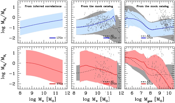
Fig. 14 Left panels: Molecular-to-atomic mass ratio, MH2 /M_HI, for LTGs (upper panel) and ETGs (lower panel) inferred from our double power-law fits to the R _HI-M_∗ and RH2 -M_∗ correlations. The shaded areas are the 1σ scatter obtained by error propagation of the scatter around the R_HI-M_∗ relations. Middle panels: Same as left panels, but from our mock catalog generated to sample the empirical GSMF, volume-complete ETG/LTG fractions as a function of mass, and R_HI-M_∗ and RH2 -M_∗ correlations. The dotted line surrounded by the gray area is the total MH2 /M_HI ratio and the 1σ scatter as a function of stellar mass. Right panels: Molecular-to-atomic mass ratio as a function of the cold gas mass, M_gas, from the mock catalog for LTGs (upper panel) and ETGs (lower panel). We plot available detected and undetected cold gas observational data as gray unfilled circles and downward arrows respectively. The color figure can be viewed online. 

According to Figure 14, the molecular-to-atomic mass ratio of LTGs increases with M_∗, albeit with a large scatter. On average, MH2 /M_HI increases from ≈ 0.1 to ≈ 0.8 for masses ranging from M_∗ = 10⁸ M_⊙ to 3 × 10¹¹ M_⊙. Given that the surface density of LTGs correlates significantly with M _∗, one can expect this dependence of MH2 /M_HI on M_∗ at least from two arguments: (1) Disk instabilities, which drive the formation of molecular clouds (e.g., the ^{Toomre criterion Toomre 1964}), are more probable to occur as the disk surface density is higher. (2) The H₂-to-HI mass ratio in galaxies has been shown to be directly related to the hydrostatic gas pressure (^{Blitz & Rosolowsky 2006}; ^{Krumholz et al. 2009}), and this pressure depends on the (gas and stellar) surface density (^{Elmegreen 1989}). In fact, the physics of H₂ condensation from HI is very complex and it is expected to be driven by local parameters of the ISM (see e.g., ^{Blitz & Rosolowsky 2006}; ^{Krumholz et al. 2009}; ^{Obreschkow & Rawlings 2009}). Therefore, the dependence of the H₂-to-HI mass ratio on M_∗ should be understood as consequence of the correlations of these parameters (their mean values along the galaxy) with M_∗, introducing this actually large scatter in the dependence of MH2 /M_HI on M_∗. Indeed, several authors have shown that MH2/M_HI correlates better with the mean gas-phase metallicity or mean stellar surface density than with M_∗ (e.g., ^{Saintonge et al. 2011}; ^{Boselli et al. 2014a}).

For ETGs, the trend of the H₂-to-HI mass ratio is inverse to the one of LTGs and shows a very large scatter. The ETGs more massive than ≈ 10¹¹ M_⊙ have mean ratios around 0.15 and a 1-σ scatter of ≈ ±1 dex; for intermediate masses, this ratio increases on average, and for ETGs with masses M∗ ≈ 109 M⊙, which are actually very rare, their mean H2-to-HI mass ratios are ≈ 1 with the same scatter of ≈ ±1 dex. Even though the gas fraction in ETGs is much smaller than in LTGs at all masses (see Figure 5), the former are also typically more compact than the latter, resulting probably in similar or higher gas pressures on average, and consequently similar or even higher MH2 /M_HI ratios, especially at masses smaller than M_∗ ≈ 10¹⁰ M_⊙. In fact, given the large scatter in MH2 /M_HI for ETGs, this ratio depends likely on many other internal and external factors (mergers, environment, etc.) that do not correlate significantly with M_∗.

Regarding MH2/M_HI vs. M_gas, for LTGs, which for M_∗ > 10⁷ M_⊙ have mostly gas masses > 108 M_⊙, there is no significant dependence, while for ETGs, which are almost inexistent with M_gas ≳ 10⁹ M_⊙, MH2/M_HI is larger on average for lower values of M_gas. This can be seen in the right panel of Figure 14, where the mock catalog has been used. Basically, for a given Mgas, in the mass range M_gas ≈ 10⁷ − 10⁹ M_⊙, ETGs have typically larger H₂-to-HI mass ratios than LTGs. In combination, the H₂-to-HI ratio appears to be larger for lower values of M _gas. Such a dependence has been reported by ^{Obreschkow & Rawlings (2009)} for their compiled sample of galaxies, and predicted by these authors for a physical model.

The dependences of the H₂-to-HI mass ratio on M_∗, M_gas, and morphological type discussed above are in qualitative agreement with several previous observational works, which actually are part of our compilation (^{Leroy et al. 2008}; ^{Obreschkow & Rawlings 2009}; ^{Saintonge et al. 2011}; ^{Boselli et al. 2014a}; ^{Bothwell et al. 2014}). However, our results extend to a larger mass range and separate explicitly the two main populations of galaxies.

7.2. The Role of Environment

There are several pieces of evidence that the atomic gas fraction of galaxies is lower in higherdensity environments (e.g., ^{Haynes & Giovanelli 1984}; ^{Gavazzi et al. 2005}; ^{Cortese et al. 2011}; ^{Catinella et al. 2013}; ^{Boselli et al. 2014c}). The fact that the ETG population has lower HI gas fractions than the LTG one (§ 4), the former being commonly found in higher-density environments, agrees with the mentioned environment trends. Thus, due to the morphology-density relation, our determinations of the R_HI-M_∗ (as well as RH2-M_∗ and R_gas-M_∗) correlations for the LTG and ETG populations, partially account for the dependence of these correlations on environment. Moreover, for the very isolated LTGs and for the subsample of LTGs in the Virgo cluster central regions, we confirm higher and lower HI-to-stellar mass ratios than the average of the overall LTG sample, respectively (see § 3.1). However, this systematic difference according to the environment is within the 1σ scatter of the R_HI-M_∗ correlation of LTGs (see Figure 3). Instead, in the case of ETGs, the isolated galaxies have much larger RHI values than the mean of all ETGs, above the 1σ scatter; isolated ETGs are almost as HI gas rich as the mean of LTGs.

Regarding the molecular gas fraction, the observational results are controversial in the literature. Recent studies seem to favor the the fact that galaxies in clusters are actually H₂-deficient compared to similar galaxies in the field. However, the deficiencies are smaller than in the case of HI (^{Boselli et al. 2014c}, and references therein). Here, for isolated and Virgo-center LTGs, we do not see any systematical segregation of RH2 from the rest of our compiled LTGs (Figure 4), but in the case of ETGs, the isolated galaxies have on average larger values of RH2.

In summary, the results from our compilation point out that the HI content of LTGs has a (weak) dependence on environment, mainly due to the fact that at high densities LTGs are HI deficient. However, the H₂ content of LTGs seems not to change on average with the environment. In the case of ETGs, those very isolated are significantly more gas rich (both in HI and H₂) than the average at a given mass.

An important aspect related to the environment is whether a galaxy is central or satellite. The local environmental effects once a galaxy becomes a satellite inside a halo. Ram pressure, viscous stripping, starvation, harassment and tidal interactions work in the direction of lowering the gas content of the galaxy, likely more the more massive the halo is (^{Boselli & Gavazzi 2006}; ^{Brown et al. 2017}). Part of the scatter in the gas-to-stellar mass correlations is probably due to the external processes produced by these local-environment mechanisms. A result in this direction has been recently shown for the R_HI-M_∗ correlation by ^{Brown et al. (2017)}. These authors have found that the HI content of satellite galaxies in more massive halos has, on average, lower HI-tostellar mass ratios at fixed stellar mass and specific SFR. According to their analysis, the systematic environmental suppression of the HI content at both fixed stellar mass and fixed specific SFR in satellite galaxies begins at halo masses typical of the group regime (> 10¹³ M_⊙), and fast-acting mechanisms such as ram-pressure stripping are suggested to explain their results. In a future study, we will attempt to characterize the central/satellite nature of our compiled galaxies, as well as calculate a proxy to their halo masses, in order to clarify this question.

7.3. Comparisons with Previous Works

In Figure 15 we compare our results with those of previous works. When necessary, the data are corrected to a ^{Chabrier (2003)} IMF. Most of the previous determinations of the HI- and H2-to-stellar mass correlations are not explicitly separated for the two main galaxy populations as done here, and in several cases non-detections are assumed to have the values of the upper limits, or are not taken into account.

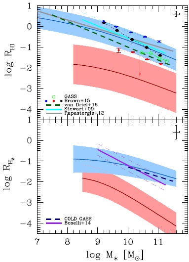
Fig. 15 Upper panel: Our empirical HI-to-stellar mass correlations for LTGs and ETGs (blue and red shaded areas, respectively) compared with some previous determinations (see labels inside the panel and details of each determination in the text). Previous determinations are based on compilations typically biased to late-type, blue galaxies, and/or do not take into account non-detections. The blue and red arrows correspond to estimates of the difference between the logarithm of the mean (the stacking technique provides the equivalent of the mean value) and the logarithmic mean (our determinations are for this case) for standard deviations of 0.52 and 0.99 dex, respectively (see text for more details). Lower panel: Our empirical molecular H₂-to-stellar mass correlations for LTGs and ETGs (blue and red shaded areas, respectively) compared with very rough previous determinations not separated into LTGs and ETGs (see labels inside the panel and details of each determination in the text). The color figure can be viewed online. 

In the upper panel, our empirical R_HI-M_∗ correlations for LTGs and ETGs are plotted along with the linear relations given by ^{Stewart et al. (2009)} (cyan line, the dashed lines show the 1σ scatter) and ^{Papastergis et al. (2012)} (gray line). The former authors used mainly the observational data presented in ^{McGaugh (2005)} for disk-dominated galaxies, and the latter authors used samples from ^{Swaters & Balcells (2002)}, ^{Garnett (2002)}, ^{Noordermeer et al. (2005)}, and ^{Zhang et al. (2009)}, which refer mostly to late-type galaxies. Their fits are slightly above the mean of our LTG R_HI-M_∗ correlation. This is likely due to their ignoring non detections. We also plot the logarithmic average values in mass bins reported by ^{Catinella et al. (2013)} for GASS (green open circles). Since ETGs progressively dominate in number as the mass increases, our total (density-weighted) R_HI-M_∗ correlation would fall below the one by ^{Catinella et al. (2013)}, especially at the largest masses. Note that for the data plotted from ^{Catinella et al. (2013)}, the HI masses of non-detections were set equal to their upper limits. Therefore, the plotted averages are biased to high values of RHI, specially for ETGs which are dominated by non-detections. Furthermore, recall that we have corrected the upper limits of GASS for distance to make them compatible with those of the nearer ATLAS^3D survey.

More recently, ^{Brown et al. (2015)} have used the HI spectral stacking technique for a volume-limited, stellar mass selected sample from the intersection of SDSS DR7, ALFALFA, and GALEX surveys. With this technique the stacked signal of co-added raw spectra of detected and non-detected galaxies (about 80% of the ALFALFA selected sample) is converted into a (lineal) average HI mass. The authors have excluded from their analysis HI-deficient galaxies - typically found within clusters- because of their significant offset to lower gas content. The black dots connected by a dotted line show the logarithm of the average R_HI values reported at different stellar mass bins in ^{Brown et al. (2015)}. Since HI-deficient galaxies -which typically are ETGs- were excluded, the ^{Brown et al. (2015)} correlation should be compared with our correlation for LTGs. Note that with the stacking technique it is not possible to obtain the population scatter in R _HI because the reported mean values come from stacked spectra instead of from averaging individual values of detections and nondetections. However, the stacking can be applied to subsets of galaxies, for example, selected by color. ^{Brown et al. (2015)} have divided their sample into three groups by their NUV−r colors: [1,3), [3,5), and [5,8]. The average RHI values at different masses corresponding to the bluest and reddest groups are reproduced in Figure 15 with the blue and red symbols, respectively. Note that the logarithmic mean is lower than the logarithm of the mean. For a lognormal distribution, log⁡x=log⁡x-0.5×σlog⁡x2 ln⁡10 (see e.g., ^{Rodríguez-Puebla et al. 2017}). Then, for the typical scatter of 0.44 dex corresponding to LTGs, the logarithm of the stacked values of R_HI should be decreased by ≈ 0.2 dex to compare formally with our reported values of logarithmic means; this is shown with a black arrow in Figure 15. If the reddest galaxies in the ^{Brown et al. (2015)} stacked sample are associated with ETGs (which is true only partially), then for them the correction to a logarithmic mean is of ≈ 1 dex, shown with a red arrow.

Finally, recently ^{van Driel et al. (2016)} reported the results for HI observations at the Nancay Radio Telescope (NRT) of 2839 galaxies selected evenly from SDSS. The authors present a Buckley-James linear regression to their data (long-dashed green line in Figure 15), taking into account this way upper limits for non-detections (though their upper limits are quite high given the low sensitivity of NRT). They fitted the entire sample, that is, they do not separate into LTG/ETG or blue/red groups. In a subsequent paper (^{Butcher et al. 2016}), the authors obtained ≈ 4 times more sensitive follow-up HI observations at Arecibo for a fraction of the galaxies that were either not detected or marginally detected; 80% of them were detected with HI masses ≈ 0.5 dex smaller than the upper limits in ^{van Driel et al. (2016)}, and the rest, mostly luminous red galaxies, were not detected. If this trend is representative of the rest of the NRT undetected galaxies, ^{Butcher et al. (2016)} expect the fit plotted in Figure 15 to be offset toward lower RHI values by about 0.17 dex and even more at the highest masses. This fit lies between a density-weighted fit to our two correlations when taking into account that at large masses the fraction of ETG/red galaxies increases and at small masses LTG/blue galaxies dominate.

The lower panel of Figure 15 is similar to the upper panel, but for the RH2-M_∗ correlations. Regarding the molecular gas content, there are only a few attempts in the literature to determine the relation between MH2 and M_∗. In fact, those works that report approximate correlations are included in our compilation: ^{Saintonge et al. (2011)} for COLD GASS, and ^{Boselli et al. (2014a)} for HRS. The former authors report a linear regression to their binned data assuming H₂ masses for non-detection set equal to their upper limits. The latter authors present a bisector fit using only detected, late-type gas-rich galaxies. Therefore, in both cases the reported relations are clearly biased to LTGs and toward high RH2 values.

The differences we find between our correlations and those plotted in Figure 15, as discussed above, can be understood on the basis of the different limitations that are present in each of the previous works. Bearing in mind these limitations we can conclude that the correlations presented here are in rough agreement with previous ones, but compared to them (i) they extend the correlations to a larger mass range, (ii) they separate explicitly galaxies into their two main populations, and (iii) they take into account adequately the non-detections.

References

Accurso, G., Saintonge, A., Catinella, B., et al. 2017, MNRAS, 470, 4750 [ Links ]
Andrews, B. H. & Martini, P. 2013, ApJ, 765, 140 [ Links ]
Avila-Reese, V., Zavala, J., Firmani, C., & Hernández-Toledo, H. M. 2008, AJ, 136, 1340 [ Links ]
Baldry, I. K., Driver, S. P., Loveday, J., et al. 2012, MNRAS, 421, 621 [ Links ]
Baldry, I. K., Glazebrook, K., & Driver, S. P. 2008, MNRAS, 388, 945 [ Links ]
Barnes, D. G., Staveley-Smith, L., de Blok, W. J. G., et al. 2001, MNRAS, 322, 486 [ Links ]
Bauermeister, A., Blitz, L., Bolatto, A., et al. 2013, ApJ, 768, 132 [ Links ]
Behroozi, P. S., Conroy, C., & Wechsler, R. H. 2010, ApJ, 717, 379 [ Links ]
Behroozi, P. S., Wechsler, R. H., & Conroy, C. 2013, ApJ, 770, 57 [ Links ]
Bell, E. F., McIntosh, D. H., Katz, N., & Weinberg, M. D. 2003, ApJS, 149, 289 [ Links ]
Bernardi, M., Meert, A., Sheth, R. K., et al. 2013, MNRAS, 436, 697 [ Links ]
Blanton, M. R., Eisenstein, D., Hogg, D. W., Schlegel, D. J., & Brinkmann, J. 2005a, ApJ, 629, 143 [ Links ]
Blanton, M. R., Lupton, R. H., Schlegel, D. J., et al. 2005b, ApJ, 631, 208 [ Links ]
Blanton, M. R. & Moustakas, J. 2009, ARA&A, 47, 159 [ Links ]
Blanton, M. R. & Roweis, S. 2007, AJ, 133, 734 [ Links ]
Blitz, L. & Rosolowsky, E. 2006, ApJ, 650, 933 [ Links ]
Blyth, S., van der Hulst, T. M., Verheijen, M. A. W., et al. 2015, Advancing Astrophysics with the Square Kilometre Array (AASKA14), 128 [ Links ]
Bolatto, A. D., Wolfire, M., & Leroy, A. K. 2013, ARA&A, 51, 207 [ Links ]
Boselli, A., Cortese, L., & Boquien, M. 2014a, A&A, 564, A65 [ Links ]
Boselli, A., Cortese, L., Boquien, M., et al. 2014b, A&A, A67 [ Links ]
Boselli, A., Cortese, L., Boquien, M., et al. 2014c, A&A, A66 [ Links ]
Boselli, A., Eales, S., Cortese, L., et al. 2010, PASP, 122, 261 [ Links ]
Boselli, A., Gavazzi, G. 2006, PASP, 118, 517 [ Links ]
Boselli, A., Lequeux, J., & Gavazzi, G. 2002, A&A, 384, 33 [ Links ]
Bothwell, M. S., Wagg, J., Cicone, C., et al. 2014, MNRAS, 445, 2599 [ Links ]
Bradford, J. D., Geha, M. C., & Blanton, M. R. 2015, ApJ, 809, 146 [ Links ]
Brown, T., Catinella, B., Cortese, L., et al. 2015, MNRAS, 452, 2479 [ Links ]
Brown, T., Catinella, B., Cortese, L., et al. 2017, MNRAS, 466, 1275 [ Links ]
Bruzual, G. & Charlot, S. 2003, MNRAS, 344, 1000 [ Links ]
Buckley, J. & James, I. 1979, Biometrika, 66, 429 [ Links ]
Butcher, Z., Schneider, S., van Driel, W., Lehnert, M. D., & Minchin, R. 2016, A&A, 596, A60 [ Links ]
Cappellari, M., Emsellem, E., Krajnovic, D., et al. 2011, MNRAS, 413, 813 [ Links ]
Carilli, C. L. & Rawlings, S. 2004, NAR, 48, 979 [ Links ]
Catinella, B., Schiminovich, D., Cortese, L., et al. 2013, MNRAS, 436, 34 [ Links ]
Catinella, B., Schiminovich, D., Kauffmann, G., et al. 2012, A&A, 544, A65 [ Links ]
Chabrier, G. 2003, PASP, 115, 763 [ Links ]
Conroy, C. 2013, ARA&A, 51, 393 [ Links ]
Conroy, C. & Wechsler, R. H. 2009, ApJ, 696, 620 [ Links ]
Cortese, L., Boissier, S., Boselli, A., et al. 2012, A&A, 544, A101 [ Links ]
Cortese, L., Catinella, B., Boissier, S., Boselli, A., & Heinis, S. 2011, MNRAS, 415, 1797 [ Links ]
Deng, X.-F. 2013, Research in Astronomy and Astrophysics, 13, 651 [ Links ]
Dressler, A. 1980, ApJ, 236, 351 [ Links ]
D’Souza, R., Vegetti, S., & Kauffmann, G. 2015, MNRAS, 454, 4027 [ Links ]
Duffy, A. R., Kay, S. T., Battye, R. A., et al. 2012, MNRAS, 420, 2799 [ Links ]
Elmegreen, B. G. 1989, ApJ, 338, 178 [ Links ]
Feigelson, E. D. & Babu, G. J. 2012, Modern Statistical Methods for Astronomy: With R Applications (Cambridge) [ Links ]
Feigelson, E. D. & Nelson, P. I. 1985, ApJ, 293, 192 [ Links ]
Fioc, M. & Rocca-Volmerange, B. 1997, A&A, 326, 950 [ Links ]
Fu, J., Guo, Q., Kauffmann, G., & Krumholz, M. R. 2010, MNRAS, 409, 515 [ Links ]
Fukugita, M., Nakamura, O., Okamura, S., et al. 2007, AJ, 134, 579 [ Links ]
Garnett, D. R. 2002, ApJ, 581, 1019 [ Links ]
Gavazzi, G., Boselli, A., van Driel, W., & O’Neil, K. 2005, A&A, 429, 439 [ Links ]
Geha, M., Blanton, M. R., Masjedi, M., & West, A. A. 2006, ApJ, 653, 240 [ Links ]
Geha, M., Blanton, M. R., Yan, R., & Tinker, J. L. 2012, ApJ, 757, 85 [ Links ]
Giovanelli, R., Haynes, M. P., Kent, B. R., et al. 2005, AJ, 130, 2598 [ Links ]
Glover, S. C. O. & Mac Low, M.-M. 2011, MNRAS, 412, 337 [ Links ]
Haynes, M. P. & Giovanelli, R. 1984, AJ, 89, 758 [ Links ]
Haynes, M. P., Giovanelli, R., Martin, A. M., et al. 2011, AJ, 142, 170 [ Links ]
He, Y. Q., Xia, X. Y., Hao, C. N., et al. 2013, ApJ, 773, 37 [ Links ]
Helfer, T. T., Thornley, M. D., Regan, M. W., et al. 2003, ApJS, 145, 259 [ Links ]
Hernández-Toledo, H. M., Vázquez-Mata, J. A., Martínez-Vázquez, L. A., Choi, Y.-Y., & Park, C. 2010, AJ, 139, 2525 [ Links ]
Huang, S., Haynes, M. P., Giovanelli, R., & Brinchmann, J. 2012a, ApJ, 756, 113 [ Links ]
Huang, S., Haynes, M. P., Giovanelli, R., et al. 2012b, AJ, 143, 133 [ Links ]
Huang, S., Haynes, M. P., Giovanelli, R., et al. 2014, ApJ, 793, 40 [ Links ]
Huertas-Company, M., Aguerri, J. A. L., Bernardi, M., Mei, S., & Sánchez Almeida, J. 2011, A&A, 525, A157 [ Links ]
Jansen, R. A., Fabricant, D., Franx, M., & Caldwell, N. 2000a, ApJS, 126, 331 [ Links ]
Jansen, R. A., Franx, M., Fabricant, D., & Caldwell, N. 2000b, ApJS, 126, 271 [ Links ]
Johnston, S., Taylor, R., Bailes, M., et al. 2008, Experimental Astronomy, 22, 151 [ Links ]
Jones, M. G., Haynes, M. P., Giovanelli, R., & Moorman, C. 2018, MNRAS [ Links ]
Jones, M. G., Papastergis, E., Haynes, M. P., & Giovanelli, R. 2016, MNRAS, 457, 4393 [ Links ]
Kannappan, S. J. & Gawiser, E. 2007, ApJ, 657, L5 [ Links ]
Kannappan, S. J., Guie, J. M., & Baker, A. J. 2009, AJ, 138, 579 [ Links ]
Kannappan, S. J., Stark, D. V., Eckert, K. D., et al. 2013, ApJ, 777, 42 [ Links ]
Kaplan, E. L. & Meier, P. 1958, Journal of the American Statistical Association, 53, 457 [ Links ]
Karachentsev, I. D., Kaisina, E. I., & Makarov, D. I. 2014, AJ, 147, 13 [ Links ]
Karachentsev, I. D., Makarov, D. I., & Kaisina, E. I. 2013, AJ, 145, 101 [ Links ]
Kauffmann, G., Heckman, T. M., White, S. D. M., et al. 2003, MNRAS, 341, 54 [ Links ]
Kauffmann, G., White, S. D. M., Heckman, T. M., et al. 2004, MNRAS, 353, 713 [ Links ]
Kennicutt, Jr., R. C., Armus, L., Bendo, G., et al. 2003, PASP, 115, 928 [ Links ]
Keres, D., Yun, M. S., & Young, J. S. 2003, ApJ, 582, 659 [ Links ]
Klypin, A., Karachentsev, I., Makarov, D., & Nasonova, O. 2015, MNRAS, 454, 1798 [ Links ]
Kravtsov, A., Vikhlinin, A., & Meshscheryakov, A. 2014, ApJ submitted, (arXiv:1401.7329) [ Links ]
Kroupa, P. 2001, MNRAS, 322, 231 [ Links ]
Kroupa, P., Tout, C. A., & Gilmore, G. 1993, MNRAS, 262, 545 [ Links ]
Krumholz, M. R., McKee, C. F., & Tumlinson, J. 2009, ApJ, 693, 216 [ Links ]
Lagos, C. D. P., Baugh, C. M., Lacey, C. G., et al. 2011, MNRAS, 418, 1649 [ Links ]
Lagos, C. d. P., Crain, R. A., Schaye, J., et al. 2015, MNRAS, 452, 3815 [ Links ]
Lagos, C. d. P., Davis, T. A., Lacey, C. G., et al. 2014, MNRAS, 443, 1002 [ Links ]
Lee, E. T. & Wang, J. W. 2003, Statistical Methods for Survival Data Analysis, (New York, NY: Wiley) [ Links ]
Lemonias, J. J., Schiminovich, D., Catinella, B., Heckman, T. M., & Moran, S. M. 2013, ApJ, 776, 74 [ Links ]
Leroy, A. K., Walter, F., Brinks, E., et al. 2008, AJ, 136, 2782 [ Links ]
Lisenfeld, U., Espada, D., Verdes-Montenegro, L., et al. 2011, A&A, 534, A102 [ Links ]
Maddox, N., Hess, K. M., Obreschkow, D., Jarvis, M. J., & Blyth, S.-L. 2015, MNRAS, 447, 1610 [ Links ]
Mandelbaum, R., Seljak, U., Kauffmann, G., Hirata, C. M., & Brinkmann, J. 2006, MNRAS, 368, 715 [ Links ]
Mandelbaum, R., Wang, W., Zu, Y., et al. 2016, MNRAS, 457, 3200 [ Links ]
Martin, A. M., Papastergis, E., Giovanelli, R., et al. 2010, ApJ, 723, 1359 [ Links ]
McGaugh, S. S. 2005, ApJ, 632, 859 [ Links ]
Meert, A., Vikram, V., & Bernardi, M. 2016, MNRAS, 455, 2440 [ Links ]
Mendel, J. T., Simard, L., Palmer, M., Ellison, S. L., & Patton, D. R. 2014, ApJS, 210, 3 [ Links ]
Meyer, M. J., Zwaan, M. A., Webster, R. L., Staveley Smith, L., Ryan-Weber, E., Drinkwater, M. J., Barnes, D. G., et al. 2004, MNRAS, 350, 1195 [ Links ]
Moffett, A. J., Ingarfield, S. A., Driver, S. P., et al. 2016, MNRAS, 457, 1308 [ Links ]
More, S., van den Bosch, F. C., Cacciato, M., et al. 2011, MNRAS, 410, 210 [ Links ]
Moster, B. P., Naab, T., & White, S. D. M. 2013, MNRAS, 428, 3121 [ Links ]
Moster, B. P., Somerville, R. S., Maulbetsch, C., et al. 2010, ApJ, 710, 903 [ Links ]
Moustakas, J., Coil, A. L., Aird, J., et al. 2013, ApJ, 767, 50 [ Links ]
Moustakas, J., Zaritsky, D., Brown, M., et al. 2011, arXiv:1112.3300 [ Links ]
Narayanan, D., Krumholz, M. R., Ostriker, E. C., & Hernquist, L. 2012, MNRAS, 421, 3127 [ Links ]
Noordermeer, E., van der Hulst, J. M., Sancisi, R., Swaters, R. A., & van Albada, T. S. 2005, A&A, 442, 137 [ Links ]
Obreschkow, D. & Rawlings, S. 2009, MNRAS, 394, 1857 [ Links ]
Papastergis, E., Cattaneo, A., Huang, S., Giovanelli, R., & Haynes, M. P. 2012, ApJ, 759, 138 [ Links ]
Paturel, G., Petit, C., Prugniel, P., et al. 2003, VizieR Online Data Catalog, 7237, 0 [ Links ]
Pforr, J., Maraston, C., & Tonini, C. 2012, MNRAS, 422, 3285 [ Links ]
Press, W. H., Teukolsky, S. A., Vetterling, W. T., & Flannery, B. P. 1996, Numerical Recipes in Fortran 90: The Art of Parallel Scientific Computing (New York, NY: CUP) [ Links ]
Rodríguez-Puebla, A., Avila-Reese, V., & Drory, N. 2013, ApJ, 767, 92 [ Links ]
Rodríguez-Puebla, A., Avila-Reese, V., Yang, X., et al. 2015, ApJ, 799, 130 [ Links ]
Rodríguez-Puebla, A., Primack, J. R., Avila-Reese, V., & Faber, S. M. 2017, MNRAS, 470, 651 [ Links ]
Saintonge, A., Kauffmann, G., Kramer, C., et al. 2011, MNRAS, 415, 32 [ Links ]
Salim, S., Rich, R. M., Charlot, S., et al. 2007, ApJS, 173, 267 [ Links ]
Sánchez, S. F., Rosales-Ortega, F. F., Jungwiert, B., et al. 2013, A&A, 554, A58 [ Links ]
Schruba, A., Leroy, A. K., Walter, F., et al. 2012, AJ, 143, 138 [ Links ]
Serra, P., Oosterloo, T., Morganti, R., et al. 2012, MNRAS, 422, 1835 [ Links ]
Simard, L., Mendel, J. T., Patton, D. R., Ellison, S. L., & McConnachie, A. W. 2011, ApJS, 196, 11 [ Links ]
Somerville, R. S. & Davé, R. 2015, ARA&A, 53, 51 [ Links ]
Springob, C. M., Haynes, M. P., Giovanelli, R., & Kent, B. R. 2005, ApJS, 160, 149 [ Links ]
Stark, D. V., Kannappan, S. J., Wei, L. H., et al. 2013, ApJ, 769, 82 [ Links ]
Stewart, K. R., Bullock, J. S., Wechsler, R. H., & Maller, A. H. 2009, ApJ, 702, 307 [ Links ]
Swaters, R. A. & Balcells, M. 2002, A&A, 390, 863 [ Links ]
Toomre, A. 1964, ApJ, 139, 1217 [ Links ]
van Driel, W., Butcher, Z., Schneider, S., et al. 2016, A&A, 595, A118 [ Links ]
Verheijen, M. A. W. 1997, PhD thesis, Univ. Groningen, The Netherlands [ Links ]
Walter, F., Brinks, E., de Blok, W. J. G., et al. 2008, AJ, 136, 2563 [ Links ]
Wei, L. H., Kannappan, S. J., Vogel, S. N., & Baker, A. J. 2010, ApJ, 708, 841 [ Links ]
Welch, G. A., Sage, L. J., & Young, L. M. 2010, ApJ, 725, 100 [ Links ]
Willick, J. A., Strauss, M. A., Dekel, A., & Kolatt, T. 1997, ApJ, 486, 629 [ Links ]
Wolfire, M. G., Hollenbach, D., & McKee, C. F. 2010, ApJ, 716, 1191 [ Links ]
Wright, A. H., Robotham, A. S. G., Driver, S. P., et al. 2017, MNRAS, 470, 283 [ Links ]
Yang, X., Mo, H. J., van den Bosch, F. C., et al. 2007, ApJ, 671, 153 [ Links ]
Young, J. S., Xie, S., Tacconi, L., et al. 1995, ApJS, 98, 219 [ Links ]
Young, L. M., Bureau, M., Davis, T. A., et al. 2011, MNRAS, 414, 940 [ Links ]
Zhang, W., Li, C., Kauffmann, G., et al. 2009, MNRAS, 397, 1243 [ Links ]
Zibetti, S., Charlot, S., & Rix, H.-W. 2009, MNRAS, 400, 1181 [ Links ]
Zu, Y. & Mandelbaum, R. 2015, MNRAS, 454, 1161 [ Links ]
Zwaan, M. A., Meyer, M. J., Staveley-Smith, L., & Webster, R. L. 2005, MNRAS, 359, L30 [ Links ]
A.The compiled galaxy samples with hi information
A.1. Golden Category
Updated Nearby Galaxy Catalog (UNGC; Karachentsev et al. 2013, 2014): It is the most representative and homogeneous sample of galaxies (869, most of them of small masses) in the Local Volume, located within 11 Mpc or with corrected radial velocities V LG < 600 Km s−1. The authors mention that the sample is complete to MB ≈ −11 mag, spanning all morphologies. However, we take a more conservative limit, bearing in mind that at low luminosities the fraction of hard-to-detect low surface brightness (LSB) galaxies strongly increases. Karachentsev et al. (2013) report the mean B−band surface brightness (SB) within the Holmberg isophote, μ-B-26 for the UNGC galaxies. The SB decreases on average with decreasing luminosity. For LTGs, the distribution of SBs appears to be incomplete from MB ≈ −13.5 mag, in such a way that most of the galaxies could be lost at lower luminosities. This is in agreement with the completeness limit suggested by Klypin et al. (2015) for UNGC, based on the turnover of the luminosity function constructed by them. In view of these arguments, we consider complete the UNGC sample for LTGs only to MB ≈ −13.5 mag (M ≈ 107.2−7.4 M); the few LTGs below this limit are of high SB and are expected to contain less gas than the average. Since ETGs are of higher SBs than LTGs, the SB distribution for the small fraction of them seems not to be affected even at the faintest observed luminosities, MB ≈ −11 mag. There are 561 galaxies with available HI data (for details regarding the data sources on HI fluxes, see Table 3 from Karachentsev et al. 2013); 90 of them do not satisfy our completeness limit. We estimate stellar masses from the reported K-band luminosities and B − K colors as in Avila-Reese et al. (2008), who calculated the massto-light ratios for HSB and LSB galaxies following Bell et al. (2003) and Verheijen (1997), respectively. The obtained masses (assuming a diet Salpeter IMF) were corrected to the Chabrier IMF. To separate HSB and LSB galaxies we use the reported μ-B,26, and transform it to a central surface brightness, μ0,B assuming an exponential disk. Thus, the criterion μB,0 > 22.5 mag/arcsec2 for selecting LSB galaxies corresponds to μ-B,26 > 24.6 mag/arcsec2. Karachentsev et al. (2013) apply corrections for peculiar motions in the determination of the distances of all the galaxies.
GALEX Arecibo SDSS Survey (GASS; Catinella et al. 2013): It is an optically-selected sub-sample of 760 galaxies more massive than 1010 M taken from a parent SDSS DR6 sample volume limited in the redshift range 0.025 < z < 0.05 and cross-matched with the ALFALFA and GALEX surveys. The HI information comes from followup observations carried out with the Arecibo 305 m telescope and detections taken from the ALFALFA survey or the Cornell HI digital archive. The R HI limit of the sample is well controlled: 0.015 for log(M/M) > 10.5 and up to 0.05 for smaller masses. There are 473 detections and 287 non detections; for the latter, upper limits are provided. For the morphological type, we use the Huertas Company et al. (2011) automatic classification applied to the SDSS DR7. These authors provide for each galaxy the probability of being of early type, PE, i.e., E or S0. We have tested this probability in a catalog of galaxies with careful visual morphological classification (UNAM-KIAS, see below; Hernández-Toledo et al. 2010) and found that galaxies of types T ≤ 1 are mostly those with PE > 0.65, and those with PE ≤ 0.65 correspond mostly to T > 1.8 Thus, we consider here as ETGs those with P E > 0.65, and the complement are LTGs. We find a good correlation between the ETGs and LTGs in this way defined with those defined using the concentration parameter c = R90/R50 to characterize the galaxy type, with the value of c = 2.85 for separating the LTGs from the ETGs (for the latter, it is also required to obey the color criterion NUVr > 5, Deng 2013). The stellar masses in Catinella et al. (2013) were calculated from the spectral energy distribution (SED) of the SDSS galaxies (Salim et al. 2007) assuming a Chabrier (2003) IMF.
Herschel Reference Survey - field galaxies (HRS; Boselli et al. 2010, 2014a, b, c): It is a K−band volume limited (15 ≤ D/Mpc ≤ 25 ) sample of 323 galaxies complete to Ks = −12 and −8.7 mag for LTGs and ETGs, respectively. The authors collected from the literature and homogenized HI data for 315 galaxies, and CO data for most of them. The morphological type was taken from NED or, if unavailable, from their own classification. Stellar masses were derived from i-band luminosities and g−i colors (from Cortese et al. 2012) using stellar mass-to-light ratios as given in Zibetti et al. (2009), and assuming a Chabrier IMF. The distances were corrected for peculiar motions and presence of clusters. The sample includes objects in environments of different density, from the core of the Virgo cluster, to loose groups and fairly isolated systems. To match the Golden category, we excluded the numerous galaxies from the Virgo Cluster center (regions A and B), which bias the sample toward high densities.
ATLAS3D HI sample - field ETGs (Serra et al. 2012): ATLAS3D is a sample of 166 local ETGs observed in detail with integral field unities (IFUs; Cappellari et al. 2011). The distance range of the sample is between 10 and 47 Mpc; the sample includes 39 galaxies (24% of the galaxies) from the Virgo Cluster. For the Golden category, we exclude those ETGs in the Virgo core. The sample is not complete, but after excluding the large number of Virgo core galaxies, it is expected to be representative of the local population of ETGs since the galaxies were selected from a complete volume-limited parent sample. The masses range from ≈ 109.8 to 1011.3 M; more massive galaxies are tipically not found in small volumes. We estimate stellar masses using log(M) = log(0.5)+log(L K ), where LK is the K-band luminosity inferred from the K-band absolute magnitude. The HI observations were carried out in the Westerbork Synthesis Radio Telescope (Serra et al. 2012). They used ALFALFA spectra to determine MHI upper limits using one resolution element and found that M HI limit is a factor ≈ 2 over the HI mass limit obtained with their data. The RHI detection limit increases with mass on average by more than 1.5 orders of magnitude, attaining values as low as ≈ 10−4 for the most massive systems. Because the ATLAS3D galaxies are nearby, the upper limits are much lower than in the case of the GASS galaxies in the same mass range.
A.2. Silver Category
Nearby Field Galaxy Survey (NFGS; Jansen et al. 2000a, b; Wei et al. 2010; Kannappan et al. 2013, and references therein): It is a broadly representative sample of 198 local galaxies spanning stellar masses M ≈ 108 − 1012 M and all morphological types. Morphological classification was obtained from Jansen et al. (2000b). The sample is not volume-complete; galaxies span distances from 2 to 306 Mpc. Distances were derived from the Virgo centric flow corrected velocities with respect to the centroid of the Local Group. Stellar masses were estimated using a variant of the code described in Kannappan & Gawiser (2007) and improved in Kannappan et al. (2009), which fits the SED and the integrated spectrum of a galaxy with a suite of stellar populations models. Both the diet Salpeter and the Chabrier (2003) IMFs were used. The single-dish HI fluxes for most of the galaxies were taken from the HyperLeda database (Paturel et al. 2003) or were obtained by the authors with the Green Bank Telescope (GBT) Spectrometer. The sample provides strong upper limits up to RHI ≈ 0.1; all galaxies with larger ratios are detected (139), and for the rest only upper limits are provided.
Stark et al. (2013) compilation: These authors compiled from the literature and homogenized 323 galaxies with available HI, CO, and multi-band imaging data. Most of the compiled galaxies are from the GASS, NFGS and ATLAS3D surveys described above. We use here only those galaxies that are not in these surveys (67 galaxies). The authors use morphological type to separate galaxies into two groups, coincident with our morphology criterion for ETGs and LTGs. In their compilation are included some blue compact dwarfs (BCDs). We exclude those BCDs classified as early types. The stellar masses were calculated following Kannappan et al. (2013). The optical and NIR information required for this calculation was taken from SDSS DR8 (for those galaxies outside the SDSS footprint, the BVRI photometry from the SINGS sample was used) and 2MASS, respectively.
Leroy et al. (2008) THINGS sample: It is a sample of 23 nearby, star-forming galaxies, which we associate with LTGs; 11 are dwarf, HI-dominated galaxies and 12 are large well-defined spiral galaxies. The HI information of the galaxies comes from “The HI Nearby Galaxy Survey” (THINGS, Walter et al. 2008) and was obtained with the NRAO Very Large Array (VLA). The stellar masses were calculated from 3.6 μm information taken from the Spitzer Infrared Nearby Galaxies Survey (SINGS Kennicutt et al. 2003). To convert the 3.6 μm intensity to surface stellar mass density, they used a K-to-3.6 μm calibration and adopted a fixed K−band mass-to light ratio, Υ*K = 0.5M /L, assuming a Kroupa was calculated from integrating the (2001) IMF; M surface stellar mass density.
Dwarf LTGs (Geha et al. 2006): It is a sample of 101 dwarf galaxies, 88 out of them with HI measurements and being of late type. Galaxies with absolute magnitudes M r − 5 log10 (h70 ) > −16 were selected from the low-luminosity spectroscopy catalog of Blanton et al. (2005b), based on the SDDS. Distances were estimated based on a model of the local velocity field (Willick et al. 1997). Possible selection effects related to the Blanton et al. (2005b) catalog include the fact that it does not span the full range of environments (there are no clusters), and LSB dwarfs are missed. Stellar masses were based on the optical SDSS i-band magnitude and g − r colors using the mass-to-light ratios of Bell et al. (2003). The M HI masses were obtained by Geha et al. (2006) from the HI integrated fluxes measured with the Arecibo 305 m telescope and the GBT.
ALFALFA dwarf sample (Huang et al. 2012b): It consists of 176 low HI mass dwarf galaxies from the ALFALFA survey. The galaxies were selected to have M HI < 107.7 M and HI line widths < 80 km s−1 (s-com sample). This sample is not complete in a volume-limited sense but it probes the extreme low HI mass tail of the ALFALFA survey. Stellar masses were obtained through SED fitting following Salim et al. (2007), assuming a Chabrier (2003) IMF. Only 57 out of the 176 galaxies have a stellar mass determination. These galaxies have HI detections and high gas fractions, they are dwarf irregulars.
A.3. Bronze Category
UNAM-KIAS catalog of isolated galaxies (Hernández-Toledo et al. 2010): It is a magnitude limited sample (mr > 15.2 mag) of galaxies from the SDSS DR5 that fulfill strict isolation criteria; it is composed of 1520 galaxies spanning all morphological types. The morphological classification was carried out by the authors. We searched HI information for these galaxies in HyperLeda (the 21-cm line magnitudes corrected for self-absorption, m21c). The HI masses were calculated as MHI=M=2.356 ×105dL2F21 where F21Jy Kms-1=100.417.40-m21c and dL is the luminosity distance to the galaxy in Mpc. For the HI non-detections, we searched rms noise limits in the Digital archive of HI 21 centimeter line spectra of optically selected galaxies (Springob et al. 2005), finding data only for 7 galaxies. Nondetected HI upper mass limits were estimated as MHIlim [M ] = 1.5·rms·δW, where δW is the full width HI of the HI line obtained from the Tully-Fisher relation of Avila-Reese et al. (2008) (δW = 2Vm is assumed). For LTGs (ETGs), we found 272 (24) detections and 7 (0) non-detections. Stellar masses were taken from the group catalog of Yang et al. (2007), where the Bell et al. (2003) mass-to-light ratios for a Kroupa (2001) IMF were used.
Analysis of the interstellar Medium of Isolated GAlaxies (AMIGA; Lisenfeld et al. 2011): It is a redshift-limited sample (1500 ≤ vrec [km s−1] ≤ 5000) consisting of 273 isolated galaxies with reported multi-band imaging and CO data. We perform the same procedure described above for the UNAM-KIAS sample to estimate detected and non- detected HI masses. For LTGs (ETGs) galaxies, we found 203 (11) detections. Only 4 non-detections were found, all for ETGs. The stellar masses were calculated as described above for the UNGC sample. Morphologies were obtained using higher resolution images from SDSS or their own images.
Low-mass Isolated galaxies (Bradford et al. 2015): It is a sample of 148 isolated low-mass galaxies (7 ≤ log(M/M) ≤ 9.5) drawn from the SDSS NSA catalog (see Geha et al. 2012). Isolated galaxies were defined as those without massive hosts (at least 0.5 dex more massive than the given galaxy) at projected distances less than 1.5 Mpc. HI measurements were obtained using the 305 m Arecibo and the 100 m Greenbank telescopes. Stellar masses were calculated in the NSA catalog with the correct software of Blanton & Roweis (2007), using the SDSS and GALEX photometric bands and assuming a Chabrier 2003 IMF. For the morphology, we used the Huertas-Company et al. (2011) automatic classification, following the same procedure described above for the GASS survey; a classification was obtained for 128 out of the 148 galaxies; all of them are of late type. Indeed, according to Geha et al. (2012) all the isolated low-mass galaxies in the local Universe are star forming (late-type) objects.
Herschel Reference Survey - Virgo galaxies: This is the same HRS sample described above but including only galaxies from the Virgo Cluster central regions A and B (59). Therefore, this sample is biased toward galaxies in a very high density environment.
ATLAS3D HI sample - Virgo core ETGs: This is the same ATLAS3D sample described above but taking into account account only the Virgo core ETGs (15). Therefore, this sample is biased in favorm of ETGs in a very high density environment.
B. The compiled galaxy samples with CO (H2) information
B.1. Golden Category
Herschel Reference Survey (HRS)- field galaxies: It is the same sample described in § A.1 (excluding Virgo Cluster core), with 155 galaxies with available CO information (101 detections and 54 non-detections). The authors used either compiled CO observations from the literature or they carried out their own observations with the National Radio Astronomy Observatory (NRAO) Kitt Peak 12 m telescope (Boselli et al. 2014a). A MW constant or H-band luminosity-dependent (Boselli et al. 2002) CO-to-H2 conversion factor was applied to calculate MH2.
CO Legacy Legacy Database for GASS (COLD GASS; Saintonge et al. 2011): This is a program aimed at observing CO(1-0) line fluxes with the IRAM 30 m telescope for galaxies from the GASS survey described in § A.1. From the CO fluxes, the total CO luminosities, (and hence the H2 masses) were calculated for 349 galaxies. The authors applied the MW constant CO-to-H2 conversion factor.
ATLAS3D H2 sample - field ETGs (Young et al. 2011): This is the same sample described in § A.1 (excluding the Virgo Cluster core) but with observations in CO using the IRAM 30 m Radio Telescope. The sample amounts for 243 ETGs with CO observations. The authors use the constant MW CO-to-H2 conversion factor.
B.2. Silver Category
Stark et al. (2013) compilation: It corresponds to the same compiled galaxy sample described in § A.2. The authors observed 35 galaxies of the NFGS with the IRAM 30 m and the ARO 12 m telescopes to measure the CO (J → 2 − 1) (IRAM) and (J → 1 − 0) (IRAM & ARO) lines. For the other galaxies, the H2 information from previous works was used. Stark et al. (2013) used the MW constant CO-to-H2 factor for estimating MH2.
Leroy et al. (2008) HERACLES sample: It is the same sample described in § A.2. The H2 information for the 23 galaxies (LTGs) comes from the CO J → 2−1 maps from the HERA CO-Line Extragalactic Survey HERACLES (Leroy et al. 2008). COJ →2−1 is related to COJ →1−0 by assuming the ratio ICO (2 → 1)/ICO (1 → 0) = 0.8, and CO J → 1 − 0 maps from the Berkeley-IllinoisMaryland Association (BIMA) Survey of Nearby Galaxies (BIMA SONG Helfer et al. 2003). The MW constant CO-to-H2 conversion factor was used.
APEX Low-redshift Legacy Survey for MOlecular Gas: (ALLSMOG; Bothwell et al. 2014) Using the APEX telescope, the CO(2 → 1) emission line was measured to trace H2 in 42 late- type galaxies with masses 8.5 <log(M/M)< 10, in the redshift range 0.01 < z < 0.03 and with metallicities 12 + log(O/H) > 8.5. Morphological classification was taken from NED. The stellar masses were derived by SED fitting (Kauffmann et al. 2003) using the SDSS DR7 optical data. To obtain the CO(1 → 0) line luminosities, the CO(2 → 1) emission line was assumed to be fully thermalized. A MW constant, or metallicity-dependent (Wolfire et al. 2010), CO-to-H2 conversion factor was applied to infer the H2 masses.
Bauermeister et al. (2013) compilation: We took from this literature compilation 8 galaxies in the low-redshift range 0.05 ≤ z ≤ 0.1. All of them are star forming and we associated them to LTGs. Their stellar masses are in the range 4×10¹⁰ MM ≤ 1.6 × 10¹¹ M and they were calculated by fitting SDSS ugriz photometry to a grid of models spanning a wide range of star formation histories. The H2 masses were obtained by the authors from CO J → 1 − 0 intensity maps with CARMA, using a MW constant CO-to-H2 conversion factor.
B.3. Bronze Category
Analysis of the interstellar Medium of Isolated GAlaxies (AMIGA; Lisenfeld et al. 2011): This is the same sample described in § A.3. The authors carried out their own observations of CO(J →1−0) with the IRAM 30 m or the 14 m FCRAO telescopes for 189 galaxies; 87 more were compiled from the literature. An aperture correction was applied to the CO data. A MW constant CO-to-H2 conversion factor was used to compute MH2
Herschel Reference Survey - Virgo core: This is the same HRS sample described above but including only the Virgo Cluster core regions A and B galaxies (62). Therefore, this sample is biased toward galaxies in a very high density environment.
ATLAS3D H2 sample - Virgo core ETGs: This is the same ATLAS3D sample described above but taking into account account only the Virgo core ETGs (21). Therefore, this sample is biased toward ETGs in a very high density environment.
C. The CO-to-H2 conversion factor
Several authors have shown that the CO-to-H2 conversion factor depends on the gas phase metallicity, Z (see e.g., Boselli et al. 2002; Schruba et al. 2012; Narayanan et al. 2012; Bolatto et al. 2013). In a recent review on the topic, among the several approaches for determining the dependence of αCO on Z in galaxies, Bolatto et al. (2013) recommend a prescription based on a local physical model for the H2 and CO production and calibrate it with extragalactic observations. In particular, they find that the prescription given in Wolfire et al. (2010), based on photodissociation models with shielding, is the most consistent with the scarce observational data that provide αCO vs. Z in galaxies. According to Wolfire et al. (2010):
αCO=αCO,MWexp+4.0AVZ'A-V,MWexp-4.0AVA-V,MW (C9)
where αCO,MW = 3.2 (in units M pc−2/K km s−1) is the adopted conversion factor for the Milky Way, Z′ = Z/Z where Z ≡ 12 + log10(O/H), ∆AV ≈ 1, and A-V,MW is the mean extinction through a giant molecular cloud with Milky Way metallicity Z, with A-V,WM5 for ΣGMC ≈ 100 Mpc−2. According to equation (C9), αCO ≈ αCO,MW for Z ≳ Z. The left panel of Figure 16 shows the Wolfire et al. (2010) relation along with those of Glover & Mac Low (2011) and Schruba et al. (2012).
Fig. 16 Left panel: Dependence of the CO-to-H2 factor on gas-phase metallicity as given by physical models (Wolfire et al. 2010; Glover & Mac Low 2011) calibrated by observations and by a purely empirical approach (Schruba et al. 2012). Observations do not allow to constrain these relations for metallicities lower than 12 + log10(O/H) _ 7.9 Middle panel: Dependence of metallicity on mass according to the CALIFA (Sánchez et al. 2013) and SDSS (Andrews & Martini 2013) surveys. We use an updated relation for CALIFA that includes more galaxies, especially at small masses (S. Sanchez, priv. communication); the masses were corrected from the Salpeter to the Chabrier IMF. The dotted line shows the SDSS relation lowered by 0.1 dex to correct for the aperture effect; notice how well it agrees with the CALIFA relation, but it extends to smaller masses, so this is the relation we use. Right panel: Dependence of the CO-to-H2 factor on mass inferred from the αCO-M and ZM dependences plotted in the other panels. The color figure can be viewed online.
To relate αCO to stellar mass, we use the massmetallicity relation for galaxies in the local Universe. Sánchez et al. (2013) and Andrews & Martini (2013) determined the mass-metallicity relation for galaxies using the CALIFA and SDSS surveys in the stellar mass range 8.4 ≤ log(M/M) ≤ 11.2 and 7.4 ≤ log(M/M) ≤ 11.2, respectively. The work by Sánchez et al. (2013) provides a more reliable estimate of the mass-metallicity relation; recall that the SDDS galaxies are mapped by only one central fiber of fixed aperture, while CALIFA maps the whole galaxies with many integral field units. However, the mass range in the CALIFA sample is limited, while that of Andrews & Martini (2013) extends to very low masses. We use an updated version of the CALIFA mass-metallicity relation (S. F. Sanchez, priv. communication) and correct M to pass from the Salpeter IMF to the Chabrier one used in Andrews & Martini (2013). At the mass range where both studies coincide, they agree modulo a shift in the SDSS relation by ≈ +0.1 dex in metallicity compared to the CALIFA one (see the middle panel of Figure 16). This is expected given that CALIFA covers the galaxies up to 2-3 effective radii while SDSS in most cases covers only the central regions which are typically more metallic than the outer ones (see for a discussion Sánchez et al. 2013). Thus, we use the relation as reported in Andrews & Martini (2013) but lowering it by 0.1 dex. They found that the function proposed by Moustakas et al. (2011) fits well their observational results:
12+ log10 O/H=12+log10O/Hasm-log101+MTOM*γ, (C10)
with 12+log10(O/H)asm = 8.798 (we use 8.698, after subtracting 0.1 dex), MTO = 8.901, and γ = 0.640.
Combining equations (C9) and (C10), we are able to obtain the mean αCO-M relation. In fact, the metallicity in any calibration is one of the hardest astronomical quantities to measure with precision. However, for our purpose, given the large uncertainties and scatter the exact calibration is not relevant; the average dependence of the αCO factor with mass is sufficient. Following Bolatto et al. (2013), we actually normalize the αCO-M dependence to αCO = αCO,MW at M = 3 × 10¹⁰ M, corresponding to a metallicity slightly lower than Z. For larger masses (metallicities), we assume that this value remains constant, and for smaller masses, we use the mass dependence given by the combination of equations (C9) and (C10):
logαCO=0.15+0.351+0.13×1010MM*0.64. (C11)
This equation is valid roughly down to M ≈ 108 M, which corresponds to metallicities ≈ 0.8 dex below the solar one (or 12 + log(O/H) ≈ 7.9); there are no observational determinations of αCO at lower metallicities. Therefore, for M < 108 M, we use the same value of αCO at 108 M, i.e., αCO ≈ 250. Besides, as highlighted in Bolatto et al. (2013), as one moves to increasingly low metallicities, the use of CO emission to quantify the H2 reservoir becomes increasingly an extrapolation and eventually a practical floor should appear past which CO is not a useful tracer of total H2 mass; rather, CO will be a tracer of high column density peaks and well-shielded regions.
The above αCO-M dependence is applied to LTGs. The right panel of Figure 16 shows this dependence along with those calculated from the αCO −Z dependences from Glover & Mac Low (2011) and Schruba et al. (2012). For ETGs, which typically have higher metallicities than Z, we assume αCOCO,MW = const. at all masses.
D. Corrections to the upper limits of ETGs
In § 5, we noted that the upper limits reported for the GASS (HI) and COLD GASS (H2) samples in the case of ETGs are significantly larger than those reported for the ATLAS3D or HRS samples. Following Serra et al. (2012), we corrected the ATLAS3D upper limit values by a factor of two in order to take into account differences between the different telescopes and signal-to-noise thresholds used in this survey and in GASS (see § 5). However, the main reason for the differences in the upper limits among these samples is a selection effect due to the different volumes covered by them. To illustrate this, in the left panel of Figure 17 we plot the histogram of HI masses for ETGs in the 10.10 − 10.65 log M bin for GASS (solid black line) and ATLAS3D (dotted black line). Non-detections are also included, with values of MHI corresponding to their upper limits. The red lines show the histograms of detections only. The number of GASS ETGs increases as MHI decreases and it has a peak at log(MHI /M)≈ 8.4 − 9.0, contributed mainly by the upper limits and consistent with the sensitivity limit of the ALFALFA survey at the distances of the GASS galaxies in the mentioned stellar mass range. For ATLAS3D, with distances much closer than GASS, some ETGs are detected in HI with masses lower than log(MHI/M)=8.4, but most of them are actually undetected, having upper limits 1-1.5 orders of magnitude lower than in the case of GASS, which is consistent with the distance differences between both samples. The main difference between the MHI distributions of both samples is their upper limits, and this is clearly due to a selection effect imposed by the different distance ranges of these samples. Basically, if the undetected GASS ETGs were at the distances of ATLAS3D ETGs, then probably most of them would not be detected in HI, having upper limits lower by 1-1.5 orders of magnitude. Thus, the high values of their upper limits imposed by the volume of GASS, are expected to introduce a bias in the determination of the gas-tostellar mass correlations of ETGs.
Fig. 17 Left panel: Distributions of HI masses for ETGs in the 10.10 − 10.65 log M bin for GASS (solid black line) and ATLAS3D (dashed black line). Non-detections are also included, with values of MHI corresponding to their upper limits (for ATLAS3D, we use the upper limits increased by a factor of two as explained in § 5). The red lines show the contribution of detected galaxies. The GASS distribution is clearly limited to much higher upper limits than ATLAS3D, and this is mainly due to a distance selection effect. Right panel: Same as left panel but after correcting the upper limits of GASS according to the observations of ATLAS3D. The color figure can be viewed online.
In an attempt to correct for this selection effect, we will assume that the ETGs in the GASS and ATLAS3D (and HRS, too) samples are representative of the same local ETG populations. Then, the fact that the upper limits for the ATLAS3D (or HRS) ETGs are significantly lower than those of similar stellar mass galaxies from GASS, is mainly due to the distance differences among these samples. If the GASS ETGs were as near as the ATLAS3D ones, then the upper limit region in the plots of HIto-stellar mass ratio vs. M would be on average lower by a factor equal to the squared distance ratio. Thus, to homogenize the upper limits in RHI given by the GASS and ATLAS3D samples, we decrease the upper limits of the galaxies in the volumelimited sample with more distant galaxies (GASS) by Di/D-ATLAS3D2, where Di is the distance of each GASS ETG and D-ATLAS3D = 25 Mpc is the average distance of the ATLAS3D ETGs. In fact, according to the ATLAS3D observations, 25% of ETGs below the upper limit region of GASS were detected (see for an example Figure 17). Therefore, we decrease the GASS upper limits as mentioned above for 75% of the galaxies, and for the remaining ones we assign randomly an R HI value between its upper limit and the average upper limit of the ATLAS3D galaxies at the corresponding stellar mass. The same procedure is applied to the COLD GASS ETGs for the RH2 upper limits, where the corresponding D-ATLAS3D for COLD GASS is 26 Mpc.
The right panel of Figure 17, shows the same histograms as the left panel but now the upper limits of the GASS sample are corrected as explained above. Observe how similar are now the upper limit distributions of GASS and ATLAS3D galaxies after correcting for the distance selection effect. Further, we use a large mock galaxy catalog to test the procedure applied here to the GASS (or COLD GASS) upper limits to homogenize them with those of nearby samples such as ATLAS3D. The mock catalog is a volume-limited sample (up to 313 Mpc) of 5×10⁶ galaxies that represents well the observational GSMF and LTG/ETG fractions as a function of M (see § 6). We assign HI masses to each LTG/ETG galaxy by using an input RHI distribution for a given M (a RHI-M relation and its scatter) for LTGs and ETGs. Distances are assigned assuming an isotropic distribution within a sphere of the same radius of the volume sampled. Note that we ignore any clustering properties of the galaxies. This is a safe assumption as we are only interested in the selection effects introduced by the detection limits of the GASS and ATLAS3D samples. Then, we select ETGs more massive than 1010 M in the 109 < D < 222 Mpc range (the GASS volume), and impose upper limits to the RHI ratio as a function of mass like the one of GASS (see Catinella et al. 2012). Then, we calculate the mean RHI and its standard deviation taking into account the upper limits in mass bins as we did for the observational sample (using the KaplanMeier estimator). The question now is whether we recover the input RHI-M correlation for ETGs.
In the left panel of Figure 18, we plot our input RHI-M correlation for ETGs (for this exercise, it is described by a double power-law function with the parameters given in Table 6 and assuming a log normal scatter) along with the values from the mock catalog in the 109 < D < 222 Mpc volume and imposing the sensitivity limit of the GASS sample (dots). All the dots below this limit are plotted as upper limits (blue arrows); they populate the imposed sensitivity limit in the RHI vs M diagram. The open circles with error bars are the mean and standard deviation calculated directly from the catalog in log M bins for ETGs in the 109<D<222 Mpc volume, while the magenta squares and error bars are the same means and standard deviations calculated with the Kaplan-Meier estimator after imposing the GASS sensitivity limit. Thus, after imposing this limit, the recovered correlation is far from the input one.
Fig. 18 Left panel: ETGs from our 109 < D < 222 Mpc volume mock catalog in the RHI vs. M plane, following the selection and RHI limits of GASS. All mock ETGs below the GASS RHI limits (dashed line) are assumed as undetected and assigned an RHI value equal to the RHI limit (upper limit; blue arrows). The magenta squares with error bars show the mean and standard deviation calculated in different mass bins with the Kaplan-Meier estimator. The RHI-M correlation for ETGs used in the generation of the mock catalog is plotted with the red solid line and shaded area. The circles with error bars show the mean and standard deviation calculated in different mass bins for all the ETGs from the mock catalog. The mock catalog samples very well the input correlation but this is not the case when the RHI limit of GASS is imposed, even when using the Kaplan-Meier estimator to take into account the upper limits. Right panel: Same as left panel but after applying our ATLAS3D-based corrections to the upper limits of GASS (see text). The mean and standard deviation in the different mass bins, taking into account the (corrected) upper limits, now follow closely the input correlation. The color figure can be viewed online.
Then, we apply the same corrections we have used for the real GASS data, based on the information from the ATLAS3D sample, i.e., the GASS like imposed upper limits to the mock catalog galaxies were decreased by Di2Mpc2/252Mpc2 in 75% of the cases, and for the remaining, a random detection value for RHI was assigned as explained above. The right panel of Figure 18 shows the result of these corrections along with the mean and standard deviations calculated with the corrected data in the same three mass bins as in the left panel (magenta squares with error bars). Note that after our corrections, the calculated mean and standard deviation in each mass bin are in better agreement with those corresponding to the mock catalog without any selection, that is, the input RHI-M correlation is reasonably well recovered; this shows the necessity of applying the mentioned corrections.
The effect of introducing the mentioned correction to the GASS and COLD GASS upper limits for the determination of the HI- and H2-to-stellar mass correlations of ETGs is, of course, not as significant as in the experiment shown in Figure 18 because these samples are not the only ones used (§ 2.2 and 2.3). In Tables 5 and 6 (cases ETGndc), we present the fitted HI-to-stellar mass correlation for ETGs for the case where the upper limits of the GASS sample were not corrected by distance. The double power-law correlation, without the correction, changes slightly at the large-mass end: it is shallower but with a much larger scatter than when we made the correction; the latter is expected due to the strong segregation of the upper limits from COLD GASS and from the less distant ATLAS3D and HRS samples. The single power-law would be shallower. Similarly, in these tables is also shown the fitted H2-to-stellar correlation for ETGs when the upper limits of the COLD GASS sample were not corrected by distance. The relations are actually almost the same whether or not the correction is taken into account, but the scatter is larger at the large-mass end for the latter case, as expected due to the segregation of the upper limits from COLD GASS and from the less distant ATLAS3D and HRS samples.
E. Observational errors
To provide a rough estimate of the intrinsic scataround the RHI -M and RH2 -M correlations shown in § 4.2 and 4.3, estimates of the (statistical) observational errors, σerr, in the determination of RHI and RH2 are necessary. For this, we need to know the respective observational uncertainties in the determination of the stellar, HI, and H2 masses.
Most of the observational sources included in our compilation do not report the individual errors in the determination of these masses, but they report conservative average estimates for them.
For the stellar mass, the observational errors are typically estimated to be 0.1 dex (see e.g., Conroy 2013). After homogenizing the samples to a fixed IMF (Chabrier 2003) we made the conservative assumption that other sources of systematic errors in the determination of M are negligible, see § 2.1.3. For the HI mass, a combination of the statistical errors, distance uncertainties, and errors associated with the absolute 21cm flux scale calibration accounts for a total observational error of ≈ 0.1 dex. Therefore, the average error in log RHI is ≈ 0.14 dex. For the H2 mass, most of the works used in our compilation report average observational errors of 0.2−0.25 dex. The uncertainty in the αCO parameter has been taken into account; however, it was probably significantly underestimated. In a recent review on the subject, Boselli et al. (2014a) suggest that this uncertainty is actually of the order of 0.3 dex. Thus, considering that the observational errors in the CO flux account for 30% (0.11 dex; e.g., Boselli et al. 2014a), and the uncertainty in the αCO parameter is 0.3 dex, an estimate of the typical error in log MH2 is 0.32 dex. The estimated error in log RH2 is then ≈ 0.34 dex, using an error of 0.1 dex in log M.
F. Calculation of the GSMF
Here we outline how we construct our GSMF in a large mass range following Kravtsov et al. (2014). For large masses, the SDSS-based GMSF presented in Bernardi et al. (2013) is used. These authors reanalyzed the photometry of the SDSS DR7, taking special care of the background estimate of extended luminous galaxies (see also Simard et al. 2011; He et al. 2013; Mendel et al. 2014; D’Souza et al. 2015; Meert et al. 2016); after this reanalysis, the high-end of the luminosity (mass) function becomes shallower. Their GSMF is well fitted by a Schechter + sub exponential Schechter function. For small masses, the GSMFs determined by Baldry et al. (2012, from the GAMA survey) were used. These authors analyzed low redshift samples that contain low luminosity galaxies, but a correction for surface brightness incompleteness was not applied. So, their determinations at M ≲ 108 M are actually lower limits. This GSMF is well fitted by double Schechter function. Both high and low mass GSMFs assume the Chabrier (2003) IMF to estimate M. However, the masses in Bernardi et al. (2013) were calculated using the Bell et al. (2003) mass-to-luminosity ratios, who employed the PEGASE stellar population synthesis models (Fioc & Rocca-Volmerange 1997). In Baldry et al. (2012) the masses were calculated using the Bruzual & Charlot (2003, BC03) models. Conroy (2013) has shown that the former are systematically larger than the latter by ≈ 0.10 − 0.14 dex. Therefore, for the Bernardi et al. (2013) GSMF, we decrease uniformly M by 0.12 dex to homogenize the masses to the BC03 population synthesis model.
Thus, we use a fit to the Baldry et al. (2012) combined with the Bernardi et al. (2013) GSMF fit corrected by 0.12 dex in mass to obtain a GSMF that spans from M ≈ 107 to 1012 M. The match of both fits (at the mass where the latter becomes higher than the former) takes place at M ≈ 109.3 M. The obtained GSMF is well fitted by the combination of a Schechter function and a sub exponential Schechter function. The respective parameters are given in Table 8. See Figure 12 for the plotted GSMF and its comparison to other GSMFs from the literature.