


 nueva página del texto (beta)
 Inglés (pdf)
 Artículo en XML
 Referencias del artículo
 Enviar artículo por email
 Citado por SciELO
  Similares en
SciELO
Similares en
SciELO 
 Permalink
1. INTRODUCTION
In the last years, there has been a growing interest in missions to Mars, with NASA and ESA announcing plans to visit the red planet. Several options are under consideration, including missions to the moons of Mars, which are a natural first step to explore the Martian system. To study those moons, it is important to find adequate orbits to place the spacecraft (Wiesel 1993).
One of the problems to be solved in the study of the Martian moons is that they are not massive enough to keep a spacecraft around them, even in highly perturbed closed orbits. In situations like that, the sphere of influence of each moon (Araujo et al. 2008), in the Mars-moon system, is below or just above the surface of the bodies (Gil & Schwartz, 2010). This means that missions whose main objective is to observe those bodies need to find alternatives for orbits of the spacecraft. Even the inclusion of propulsion systems to control the orbit of the spacecraft does not solve the problem for all types of missions, because the fuel expenditures to keep the spacecraft close to one of the moons are too high for most missions.
However, in models like the restricted three-body problem, circular or elliptic, there are special types of orbits that make possible missions to these small celestial bodies; they are known as “Quasi-Satellite Orbits” (QSO) (Benest 1976; Kogan 1989, 1990; Lidov & Vashkov’yak, 1993, 1994; Mikkola et al. 2006; Gil & Schwartz, 2010). These orbits allow the spacecraft to stay near the moon, but outside its sphere of influence. This means that the orbit is dominated by the central body (Mars), but it uses the weak gravity field of the moon to generate a motion that looks like an orbit around the moon. The “Distant Retrograde Orbits” (DRO) (Lam & Whiffen, 2005; Villac & Aiello, 2005; Whiffen 2003) are one type of these orbits, where the spacecraft stays in a retrograde motion at a large distance from the moon. Similar distant quasi-periodic orbits around Mercury also exist, like the ones shown in Ma & Li, (2013). Other types of orbits around moons of the Solar System can also be found in Carvalho et al. (2012) and Gomes & Domingos, (2016).
The objective of the present study is to search for QSO type of orbits around Phobos. Several aspects of this problem are considered. In the first step a search is made for those orbits, measuring the minimum, maximum and average Phobos-spacecraft distances for a fixed evolution time. This type of measurements gives to the mission designer a range of options for a practical mission to Phobos, which is an important point. In particular, emphasis is placed on finding mid-range orbits, which are the ones that keep the spacecraft at distances around 50 to 200 km from Phobos. Regarding the orbits, it is interesting to have some fluctuations in the distance Phobosspacecraft, to give different observation points for the spacecraft.
Those mid-range orbits are important because they are close enough to observe Phobos without risk of collision with the moon. They are also not much affected by the details of the inaccuracies of the irregular gravity field of Phobos (which is quite irregular) since the spacecraft does not pass too close to it. This means that the inclusion of the J2 term of the gravity field of the moon can give a good accuracy to represent those irregularities. These characteristics mean that those orbits are very good candidates to place the spacecraft at the time of arrival near Phobos. From these mid-range orbits, the spacecraft can make preliminary scientific observations before going to orbits closer to the moon, which means that some data will be collected in the worst scenario of a collision if the spacecraft gets too close to the moon. Another advantage of these mid-range orbits is that they allow some time for a better determination of the gravity field of Phobos, before making a final orbit selection for the close observations part of the mission. Good examples of orbits close to the moon, including landing options, are available in Zamaro & Biggs (2016). Other investigations related to landing options are available in Akim et al. (2009) and Tuchin (2008). In that sense, the present paper has the goal of complementing the existing literature, by showing a different view of this problem.
A mathematical model that follows the assumptions of the elliptic planar restricted three body problem (Szebehely 1967) is used to describe the motion of a spacecraft around a system formed by two other bodies. One of these bodies has the largest mass of the system, and it is called the primary body (Mars), while the other one has a much smaller mass and is called the secondary body (Phobos). These two bodies orbit around their common center of mass in elliptical orbits. The spacecraft is considered to have a negligible mass, so it does not interfere with the motion of the two primaries. Besides those forces, the effects of the non-spherical shape of Phobos and Mars are also considered. This is done by adding the J2 term of the gravity field of Phobos and Mars to the dynamics of the system. Phobos has a large value for this coefficient, of the order of 0.105, which means that it may cause perturbations in the orbital motion of the spacecraft around it. The importance of this force depends on the specific trajectory. The present paper will measure the effects of each force in detail, by integrating their individual contribution during the total trajectory, as done by Sanchez, Prado & Yokoyama, (2014) considering the gravity field of the Earth. The paper also shows a more direct measurement of the importance of the model used to search for the orbits, by making several studies considering different options for the model.
The results show maps of orbits identifying minimum, maximum and average spacecraft-Phobos distances for a given time, so the mission designer can choose the most adequate orbits for a given mission. Each trajectory can be identified by the initial conditions of the spacecraft with respect to Phobos, that is, its initial position and velocity. Several families of orbits are found, with particular characteristics.
The study is made considering Phobos at the periapsis and apoapsis of its orbit around Mars at the initial time of simulation. This point is important, because in spite of several studies looking for orbits in the Martian system, this aspect of the problem has not been considered. The results will show that there is an influence from this parameter. In this sense, the goals of the present paper are: (i) to search and classify orbits for a spacecraft travelling around Phobos, showing their main characteristics; (ii) to propose an alternative numerical method to find orbits of the type “Quasi Satellite Orbits”; (iii) to show the importance of considering the eccentricity of the orbit of Phobos and the irregular shapes of Mars and Phobos in the orbits found; (iv) to study the effects of each force present in the dynamical system, by integrating the accelerations of those forces during the whole trajectory, thus measuring the total variation of velocity delivered to the spacecraft by each force; (v) to study the effects of the initial position of Phobos in its orbit around Mars in those trajectories.
2. MATHEMATICAL MODEL
In this section, the mathematical model used in the simulations is presented, as well as some other important parameters that are measured during the simulations. After defining the forces involved in the dynamics, it is necessary to choose a criterion to classify the orbits found. The goal is not to find the best orbits, but only to show general maps that allow a mission designer to see some important parameters that can help to find the best choice, depending on the specific goals of a future mission. The study starts with the spacecraft at a given distance from Phobos, and then the trajectories are numerically integrated for a given time. The initial conditions are the position and velocity of the spacecraft at the beginning of the integration time. This choice gives the possibility of using these initial parameters to control the maximum, minimum and average distances spacecraft-Phobos during the whole natural trajectory, so as to be able to find the most adequate values for a specific mission. This information is obtained by looking at the evolution of the Phobos-spacecraft distance during the integration time. Based on these results, the orbits are classified according to by the maximum, minimum and average distances spacecraft-Phobos. From the results obtained here it is also noted that there are only small fluctuations in the minimum distances, which means that the averaged distances follow very closely the results for the maximum distances.
Let us consider Mars, Phobos and the spacecraft masses being m1, m2 and m3, respectively. The bodies M1, M2, and M3 move in the same plane, and the bodies M1 and M2 rotate around their center of mass in elliptical orbits, due only to the gravitational attraction between them. The body M3 travels around the bodies M1 and M2, influenced by their gravity fields, but it does not interfere with the motion of the primaries. Besides those Keplerian gravity forces, the non-spherical shapes of Mars and Phobos are also considered, expressed by the usual terms J2 of their gravity fields (Sanchez et al. 2009). It represents the flattening of the body. The equations of motion are shown in equations 1 and 2.
where G is the universal gravitational constant,
m1 and m2 are the masses
of the primary bodies (Mars and Phobos, respectively),
r1 and r2 are the
distances from the spacecraft to these primaries (also Mars and Phobos,
respectively),
In this work is proposed a numerical search for orbits using the equations of motion described by equations 1-2. The results can map those orbits as a function of the initial conditions. Some of them are plotted as examples. The criterion of considering the minimum, maximum and average distances to classify the orbits consists in measuring the time-history of the spacecraft-Phobos distance during the numerical integration of the orbit, starting from the given initial conditions of the spacecraft, and going up to the time limit specified for the orbit. This procedure is repeated for each orbit, generating maps that are used to classify the orbits. The average spacecraftPhobos distances (Davg) are calculated as shown in equation 3 (Prado 2015), where T is the integration time interval and r2 is the distance between the spacecraft and Phobos. The numerical method used for the integration is the eight order Runge-Kutta, with variable step size and accuracy of 10-10.
Next, the algorithm used to search for the orbits is described. Initially, an inertial reference frame is chosen where Mars and Phobos are aligned in the horizontal axis. In this system, the spacecraft lies at a certain distance from Phobos, in the horizontal axis. It is not necessary to consider situations with the spacecraft outside this line, because the orbit would be the same, at a different stage. In other words, all the orbits will cross this line, so this type of “line search” is enough to obtain all the orbits. Figure 1 shows the positions of Mars, Phobos, and the space vehicle, all of them with respect to an inertial frame. Also indicated are all the initial conditions of the spacecraft used to identify each orbit: the initial spacecraft-Phobos distance D and the components of the initial velocity, υx and υy, of the spacecraft. Based in Figure 1, it is possible to determine the initial position and velocity vectors of the spacecraft. Starting from these conditions, the trajectories are numerically integrated, using equations 1-2, over a given time. It is always verified if there is a collision between the spacecraft and Phobos. At the end of the trajectory, the minimum, maximum and average distances between the spacecraft and Phobos are obtained. Those results are then plotted, to give options for the mission designer to choose the most adequate orbits for a particular mission. It is also possible to sort the trajectories by the minimum, maximum, or average distances in ascending order, to get a more accurate location of the orbits that keeps the spacecraft at the desired distances from Phobos. Once these orbits are identified, the best conditions are used to plot the trajectories of the spacecraft, such that the main characteristics of the trajectories can be observed. They are plotted in the fixed and rotating frames, to give a complete view of the orbits.

Fig. 1 Representation of the problem involving the Mars-Phobos system and the description of the initial conditions that identify each orbit: D is the initial distance between Phobos and the spacecraft on the horizontal axis; υx and υy are the components of the initial velocity of the spacecraft.
Regarding the use of integrals to measure the effects of each force, there are several options to be considered. This concept has been used for some time now, in different forms. A first version appeared in Prado (2013), studying the problem of luni-solar perturbation of a spacecraft. Several improvements appeared in the literature afterward. It is possible to think about three types of integrals that show different aspects of the problem. These types are:
where a is the acceleration from each force involved in the dynamics,
The first type is used in the present paper, and it measures the total acceleration applied to the spacecraft. It considers the effect of forces that are in opposite directions and may cancel each other, because it uses the absolute value of the acceleration. It is interesting to compare the forces, which is the goal of the present paper.
The second type of integral measures how the forces affect directly the variation of energy of the spacecraft. When it is positive, the force is adding energy to the spacecraft. In the opposite situation, when it is negative, it is removing energy from the spacecraft. This type is useful when the main goal is to study the energy flux of the forces. It allows compensations of positive and negative effects during the trajectory.
The third type also makes compensations of positive and negative effects. It is the integral of each component of the acceleration. It indicates the more perturbed orbits. It is similar to the integral index defined in Lara (2016). This index measures the deviations of a perturbed orbit compared to a Keplerian orbit with the same initial conditions. This integral gives the delta-V that needs to be applied to keep the perturbed orbit following the Keplerian one.
This type of study was also made in Sanchez & Prado (2017), where perturbation maps were made using the first and second types of integral. The main goal was to find low disturbed regions. Similar studies are available in the literature using integrals of the accelerations to measure perturbations received by specific orbits in similar problems, like Carvalho et al. (2014), Oliveira & Prado, (2014), Oliveira et al. (2014), Prado (2014), Sanchez, Prado & Yokoyama, (2014), Santos et al. (2015), Sanchez, Howell & Prado, (2016), Short et al. (2016)). The main goal is to determine the increment of velocity delivered to the spacecraft by each force, which enables a comparative study of the importance of each of them.
3. RESULTS
The results of the simulations are now presented, for several sets of initial conditions. A initial period of 30 days for the orbits is used for most of the cases. Some orbits are integrated for longer times. In fact, this parameter can be varied according to the necessity of any particular mission. In general, 30 days is a good time for a natural trajectory, because after that time other forces that are not modeled in the dynamics can be important. Table 1 shows the numerical data for Mars and Phobos used in the simulations made here, i.e. the average diameters, masses, semi-major axis and orbital periods.
Table 1 Physical and orbital components of the martian system
| Celestial Body | Average radius (km) | GM (km3 /s2 ) | J2 | Semi-major axis (km) | Eccentricity |
|---|---|---|---|---|---|
| Mars | 3396.2 | 42828.0 | 0.00195 | - | - |
| Phobos | 11.1 | 0.0007112 | 0.105 | 9377 | 0.0151 |
Several figures are plotted, combining the different variables to identify the initial position of the spacecraft with respect to Phobos: D, υx and υy. In all of them are shown the maximum, minimum and average distances Phobos-spacecraft, plotted in color codes as a function of the initial conditions. The black regions in the figures indicate initial conditions that cause the spacecraft to collide with Phobos in less than 30 days. Using those maps it is possible to find the most interesting regions, which can be refined and extended using new sets of initial conditions, if necessary. It is also possible to draw the trajectories of the spacecraft.
To assess the role that each force plays in the spacecraft trajectory, simulations are made using a more accurate model that takes into account the eccentricity of the orbit of Phobos around Mars and the J 2 terms of the gravity fields of Phobos and Mars. The same simulations are made under a dynamics considering a circular orbit for Phobos around Mars and assuming spherical shapes for Mars and Phobos. The goal is to asses the importance of considering the more accurate model, and the results show that it is important to take into account the better model.
Then, a new and different study is made, using the integrals of the accelerations involved in the dynamics, as explained before, with the goal of showing the individual contribution of each force on the trajectory of the spacecraft.
The first results are shown in Figure 2, which contains the maximum (Dmax), minimum (Dmin) and average (Daυg) distances between spacecraft and Phobos as a function of the initial conditions D (km), in the vertical axis, and υx (km/s), in the horizontal axis, for orbits when Phobos is at the periapsis of its orbit around Mars. The initial velocity υy was fixed as −0.02 km/s. This value, as well as the ranges for D (85 to 95 km) and υx (−0.05 up to 0.05 km/s) were selected after several preliminary simulations, made using three loops for the variables D, Vx, and Vy. After this sequence of loops, the solutions with lower maximum and average distances are selected for more detailed studies. Those simulations indicated the best values that generate orbits in the range desired in the present paper. To build this figure, a limit of Dmin > 50 km was imposed, to preserve the validity of the model that considers only the J2 term to represent the irregular shape of the bodies, and to avoid trajectories with high risk of collision. This type of plots is a new way to classify the orbits, compared to the existing literature. Each point in the plot represents one orbit, with initial conditions specified by the value of D (vertical axis) and υx (horizontal axis). From these plots it is possible to see the evolution of spacecraftPhobos distances and to choose an orbit. A strong correspondence between maximum and averaged distances among the orbits is noted, with the minimum values of both of them located at the same initial conditions. This happens because Dmin usually has small values, and they are also very similar to each other, so they do not much influence the average distances. The closest orbits are obtained for υx near zero. It is also noted that there is some symmetry around this line. The minimum values for the maximum distances have D below 91 km, where the orbit goes as far as 500 km from Phobos, but maintains an average distance in the range 140 − 240 km. Above this value there are few orbits that remain close to Phobos. Regarding the minimum distances, the values which are more interesting for the mission are the ones above 50 km, as mentioned before. Figure 2(a) shows that there are several ranges above 50 km, in blue (50 to 70 km), red (70 to 90 km) and yellow (90 to 110 km). Using this technique, we can find the orbits that have Dmin above 50 km and minimum Dmax, which is an interesting criterion to choose the orbits. Other options are available, like using specific values and/or ranges for maximum and/or average distances, etc. Those orbits are interesting to place a spacecraft when arriving at the system, because they are close enough to make preliminary observations, but far enough to avoid accidental collisions. It is clear that the bottom region around υx = 0 satisfies those two constraints, having Dmin > 50 km, Dmax < 500 km and Davg < 240 km.

Fig. 2 Average, maximum and minimum distances, in km, as a function of D (km) and υx (km/s), with υy = −0.02 km/s, and considering Phobos at the periapsis of its orbit around Mars. The model assumes e = 0.0151,
Table 2 shows the numerical details of the five orbits that are closer to Phobos (minimum Dmax). It can be seen that they are all good candidates to place a spacecraft, keeping the vehicle in the range 84-217 km from Phobos during 30 days, without orbital maneuvers. Equivalent results using a model that considers the orbit of Phobos around Mars as circular and the bodies as spherical are also shown in Table 2, represented by an asterisk (∗). The goal is to show the importance of using the more accurate model. From those values, it is clear that the assumption of circular orbits and spherical bodies introduces errors of the order of 1 to 7 km for the minimum distances, 6 to 9 km for the averaged distances, and 11 to 30 km for the maximum distances, for the 30 days simulations. The last column of Table 2 shows positive and negative results, so the simple model may over-or underestimate the maximum distances.
Table 2 the five orbits with smaller Dmax around Phobos.†
| D (km) | υ x (km/s) | Daυg (km) | D min (km) | Dmax (km) |
(km) |
(km) |
(km) |
(km) |
(km) |
(km) |
|---|---|---|---|---|---|---|---|---|---|---|
| 88 | 0 | 141.6562 | 85.6517 | 209.1972 | 132.9068 | 84.7235 | 197.9696 | 8.7495 | 0.9281 | 11.2276 |
| 88 | -0.001 | 141.9264 | 85.6110 | 211.9005 | 133.1352 | 84.6713 | 199.6546 | 8.7912 | 0.9397 | 12.2458 |
| 88 | 0.001 | 141.9195 | 85.5839 | 212.1728 | 133.1643 | 84.6714 | 199.6519 | 8.7553 | 0.9124 | 12.5209 |
| 89 | 0 | 139.7691 | 83.9968 | 215.0385 | 133.8995 | 77.4377 | 228.8564 | 5.8696 | 6.5591 | -13.8179 |
| 89 | -0.001 | 140.0485 | 83.9250 | 216.7511 | 134.1053 | 77.3889 | 229.7915 | 5.9431 | 6.5361 | -13.0403 |
†Assuming υy = -0.02 km/s, Phobos
initially at periapsis, with e = 0.0151,
Another aspect to be considered when looking at the effects of using a simplified model for
the problem is to see what happens when the search for the orbits is made using the
simple model from the beginning. In this case, the results would be different and
the initial conditions of the orbits with smaller values for
Dmax would be different. Table 3 shows the results, with a comparison
with the same orbits obtained using the better model. It is clear that different
initial conditions are found. Using the better model, the initial conditions for the
orbit with minimum Dmax are
D = 88 km and υx =0km/s, with a maximum distance
spacecraft-Phobos of 209.2972 km after 30 days. Using the circular and spherical
model, the initial conditions for the orbit with minimum
Dmax are D = 86 km and
υx =0km/s, with a maximum distance spacecraft-Phobos of 188.3397 km
after 30 days. Then, refining this orbit with the better model, the maximum distance
spacecraft-Phobos goes to 213.1525 km after 30 days. Table 3 shows this analysis for the five orbits with smaller
Dmax (km) assuming υy =
−0.02 km/s, a circular orbit for Phobos and a spherical model for the bodies, for a
simulation time of 30 days. Equivalent results for the better model (elliptical and
flat bodies) are represented by
Table 3 The five orbits with smaller Dmax around Phobos.*
| D (km) | υx (km/s) | Daυg (km) | Dmin (km) | Dmax (km) |
(km) |
(km) |
(km) |
(km) |
(km) |
(km) |
|---|---|---|---|---|---|---|---|---|---|---|
| 86 | 0 | 133.0967 | 85.9801 | 188.3397 | 138.0525 | 83.3301 | 213.1525 | -4.9558 | 2.6501 | -24.8128 |
| 86 | -0.001 | 133.3284 | 85.9394 | 190.6564 | 139.9188 | 85.0339 | 206.6250 | -6.5904 | 0.9055 | -15.9686 |
| 86 | 0.001 | 133.3345 | 85.9419 | 190.6572 | 139.8977 | 84.9882 | 206.6556 | -6.5632 | 0.9537 | -15.9984 |
| 87 | 0 | 131.6331 | 84.6318 | 190.7846 | 138.3292 | 76.4661 | 244.8232 | -6.6961 | 8.1657 | -54.0386 |
| 87 | 0.001 | 131.8924 | 84.6044 | 192.7038 | 138.5691 | 76.3140 | 246.3559 | -6.6768 | 8.2904 | -53.6521 |
*Assuming υy = -0.02 km/s, circular orbit for Phobos and spherical model for the bodies; T = 30 days. Corresponding results for the elliptical and flat bodies are represented by
A more detailed study, considering all the perturbations (individually and combined in parts) was made. All of them showed results that are different from the ones obtained with the better model. The results indicated small differences when assuming a spherical body for Phobos, of the order of only 20 to 70 meters. The larger differences, of the order of 35 to 42 km, are related to the assumption of circular motion for Phobos. This is explained by the large eccentricity of Phobos and the small effects of the gravity of Phobos, hence the effects of J2 are also small. This means that the eccentricity of Phobos has more important effects than the non-spherical shape of the moon, and needs to be considered in the model in any situation.
Next, the test of the integrals mentioned before is made, to show the importance of each term included in the dynamics. The relative importance of each force in the evolution of the orbits is assessed by integrating the acceleration from each force individually over the time, divided by the total integration time. It is a study very similar to the one of Sanchez et al. (2014). An integration of the magnitude of the acceleration from each force is made along the trajectory, with the total result divided by the integration time. This study gives the average magnitude of each force during the whole trajectory and shows the relative importance of each force. It is an alternative form to measure the importance of each model used to approach this problem.
Figure 3 shows the values of the contribution
of Phobos, in km/s2, assuming that Phobos is at the periapsis when the
orbits start, e = 0.0151,

Fig. 3 Integral over time of the force arising from Phobos, in km/s2, as a function of D (km) and υx (km/s). The color figure can be viewed online.
To gain an idea of the temporal evolution of the orbit, Table
4 presents the values of distances (km) and perturbations
(km/s2) for the same set of initial conditions: Phobos at periapsis,
D = 88 km, υx = 0, υy = −0.02 km/s,
considering e = 0.0151,
Table 4 Temporal evolution of orbits.*
| T (days) | 5 | 15 | 30 | 60 | 90 |
|---|---|---|---|---|---|
| Daυg (km) | 136.2299 | 142.7226 | 141.6562 | 141.7514 | 141.8742 |
| Dmin (km) | 86.0742 | 86.0742 | 85.6517 | 85.6517 | 85.6517 |
| Dmax (km) | 192.5870 | 209.1972 | 209.1972 | 209.1972 | 209.1972 |
| PertPhobos 10-8 (km/s2) | 4.1650549 | 3.7458791 | 3.8230917 | 3.8112248 | 3.8056164 |
| PertMars 10-4 (km/s2) | 4.3813385 | 1.3819384 | 4.3815682 | 4.3813763 | 4.3813033 |
| Pert J2Phobos 10-11 (km/s2) | 6.4957046 | 5.3567171 | 5.5527058 | 5.5046893 | 5.5527058 |
| PertJ2Mars 10-7 (km/s2) | 1.6886343 | 1.6902662 | 1.6898772 | 1.6898200 | 1.6898156 |
*Using Phobos at periapsis, D = 88 km,
υx = 0,
υy = -0.02 km/s,
considering e = 0.0151,
Figures 4 and 5 show the trajectories corresponding to the values marked in Table 4 for the times of 5, 15, 30, 60 and 90 days, as viewed from the fixed and rotating reference systems. In all figures Phobos is considered to be at the origin of the reference system and its dimension is represented, in scale, as a gray circle.
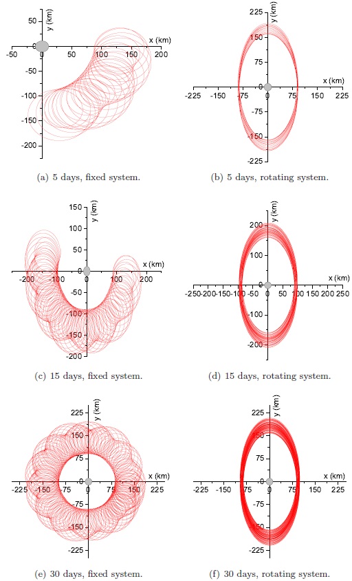
Fig. 4 Time evolution of trajectories obtained using Phobos at periapsis, D = 88 km, υx = 0, υy = −0.02 km/s, considering e = 0.0151,

Fig. 5 Time evolution of trajectories obtained using Phobos at periapsis, D = 88 km, υx = 0, υy = −0.02 km/s, considering e = 0.0151,
The next step is to evaluate the influence of the initial position of Phobos in its orbit around Mars, which is one of the goals of the present research. To perform this task, simulations are made assuming now that Phobos is in the apoapsis of its orbit around Phobos. Figure 6 and Table 5 show the results. Figure 6 is clearly different from Figure 2, which indicates the importance of the initial position of Phobos in these orbits. The large reduction of ranges of initial conditions that generate orbits with smaller maximum distances is noted. The range for maximum distances below 690 km is much larger in Figure 2(b) (blue and red regions), showing orbits with D in the range from 90 to 85 km that have maximum distances below 690 km, the majority of them with D max below 500 km. On the other hand, Figure 6(b) shows that only values of D < 87 km present orbits in this region, so restricting the range of initial conditions. The plots for the average distances have the same behavior. Differences in the behavior for the minimum distances are smaller, which means that the differences in the maximum distances are much more influenced by the initial position of Phobos in its orbit. Table 5 shows a more detailed comparison. The orbits with smaller maximum distances shown in Table 2 (Phobos initially at periapsis) have initial conditions with D = 88 or 89 km, υx of 0 or ±0.001 km/s and values of maximum distances in the interval 209 to 217 km. Table 5 (Phobos at apoapsis) shows initial conditions with D = 85 or 86 km, υx of 0, ±0.001 or 0.002 km/s and values of maximum distances in the interval 203 to 214 km. A summary of the conclusions shows that Phobos at periapsis gives a large range of initial conditions for orbits with relatively smaller values of the maximum distance, but the values are a little higher compared to the situation when it is at the apoapsis.
Table 5 The five orbits with smaller D max around Phobos.†
|
D (km) |
υx (km/s) |
Daυg (km) |
D
min (km) |
Dmax (km) |
(km) |
(km) |
(km) |
(km) |
(km) |
(km) |
|---|---|---|---|---|---|---|---|---|---|---|
| 85 | 0 | 139.6459 | 85.0780 | 203.5173 | 136.8380 | 81.4455 | 227.6470 | 2.8079 | 3.6325 | -24.1297 |
| 85 | -0.001 | 139.9188 | 85.0339 | 206.6250 | 137.0709 | 81.4006 | 228.5953 | 2.8480 | 3.6333 | -21.9704 |
| 85 | 0.001 | 139.8977 | 84.9882 | 206.6556 | 137.0613 | 81.3989 | 228.5130 | 2.8364 | 3.5893 | -21.8574 |
| 86 | 0 | 138.0525 | 83.3301 | 213.1525 | 133.0967 | 85.9801 | 188.3397 | 4.9558 | -2.6501 | 24.8128 |
| 85 | 0.002 | 140.6772 | 84.8881 | 213.9856 | 137.7604 | 81.2624 | 231.2942 | 2.9168 | 3.6257 | -17.3086 |
†Assuming υy = -0.02 km/s, Phobos initialy at
apoapsis, with e = 0.0151,
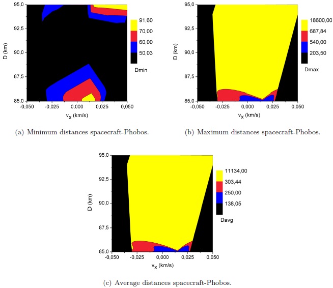
Fig. 6 Average, maximum and minimum distances, in km, as a function of D (km) and υx (km/s), considering υy = −0.02 km/s, with Phobos at apoapsis of its orbit around Mars. The model considers e = 0.0151,
From Table 5, it is noted that the assumption of circular orbits and spherical bodies introduces errors of the order of 3 to 4 km for the minimum distances, 3 to 5 km for the averaged distances and 17 to 25 km for the maximum distances, for 30 days of simulation. The last column of Table 5 shows positive and negative results, so the simple model may overor underestimate the maximum distances. Compared to similar results obtained when Phobos is initially at periapsis (Table 2), note the occurrence of larger errors arising from the two different models in the present geometry, in terms of maximum distances, with the opposite happening for minimum and average distances.
Figure 7 shows the first trajectory listed in Table 5 over 30 days, in the fixed and rotating reference systems. In all figures Phobos is considered to be at the origin of the reference system and its dimensions are presented in scale. Table 6 shows the values during the time evolution, just to confirm the stabilization of the parameters involved. The nomenclature is the same used in Table 4. For Figures 7(a) and 7(b) we have used the better model, while for Figures 7(c) and 7(d) we have used the model with a circular orbit for Phobos and spherical bodies for Mars and Phobos. The trajectories plotted in the fixed system show that the better model generates a trajectory that stays in a more limited space, while the trajectories plotted in the rotating system show that the better model generates a trajectory that moves the periapsis of the orbit faster.

Fig. 7 Trajectories considering an elliptical orbit for Phobos and flat bodies for Mars and Phobos (red) and considering a circular orbit for Phobos and spherical bodies for Mars and Phobos (blue). Phobos initially at apoapsis, D = 85 km, υx = 0, υy = −0.02 km/s, T = 30 days. The color figure can be viewed online.
Table 6 Temporal evolution of orbits using Phobos at periapsis.*
| T (days) | 5 | 15 | 30 | 60 | 90 |
|---|---|---|---|---|---|
| Daυg (km) | 135.0333 | 141.0392 | 139.6457 | 139.8844 | 140.1496 |
| Dmin (km) | 85.0780 | 85.0780 | 85.0780 | 85.0780 | 85.0780 |
| Dmax (km) | 192.7250 | 203.5173 | 203.5173 | 203.8044 | 204.1091 |
| PertPhobos 10-8 (km/s2) | 4.2267095 | 3.8291000 | 3.9322040 | 3.9025116 | 3.8919564 |
| PertMars 10-4 (km/s2) | 4.3825841 | 4.3819841 | 4.3819058 | 4.3817239 | 4.3816137 |
| PertJ2Phobos 10-11 (km/s2) | 6.6841480 | 5.5851724 | 5.8522808 | 5.7828430 | 5.7462664 |
| PertJ2Mars 10-7 (km/s2) | 1.6895451 | 1.6902093 | 1.6900063 | 1.6899644 | 1.6899568 |
*D = 85 km, υx = 0,
υy = -0.02 km/s,
considering e = 0.0151,
4. CONCLUSION
This work presents several orbits around Phobos that can be used by a spacecraft visiting the system. A new type of mapping is proposed, classifying the orbits around Phobos according to minimum, maximum and average distances Phobos-spacecraft for a given time, as a function of the initial conditions of the orbits. The results are shown in color maps depicting these parameters as a function of the initial conditions. This technique is efficient to find midrange orbits around Phobos, with Mars dominating the dynamics, while Phobos makes small perturbations that keep the spacecraft close to it. Those midrange orbits can be used to place a spacecraft when it is arriving at the system, to avoid orbits that are too close to the moon that may have a high risk of collision. They are also good choices because it is not necessary to know the shape of Phobos in much detail. The spacecraft can be transferred from those orbits to closer ones, after a better determination of the gravity field of the moon is obtained, so as to define the best final orbits for the spacecraft.
Several orbits with Phobos-spacecraft distances ranging from 50 km to near 200 km were found, for 30 days of simulations, without orbital maneuvers. The time of 30 days was considered to be good enough to make the first observations of the moon, but different values can be used with the technique presented here. Some of the more interesting orbits were studied for longer times, up to 90 days.
Particular attention is given in the effect of the initial position of Phobos in its orbit around Mars in those orbits, with the results showing that when Phobos is at periapsis, there is a large range of initial conditions for orbits with small values of the maximum distance, but the values are a little higher compared to the situation where Phobos is initially at apoapsis.
Another point studied in the present paper is the importance of the mathematical model used to represent the system. A dynamics including the J2 term of the gravity field of Phobos and the eccentricity of its orbit around Mars was used. Similar simulations were made assuming a spherical form for the moon and a spherical form and circular orbits for the moons around Mars. They showed errors of the order of a few tens of kilometers. The circular and spherical model always underestimates the value of Dmax for the orbits closer to Phobos. But even with those small errors, simplified models should be avoided, since they predict collisions in situations where they do not occur using the more accurate model that includes the J2 term from the moon and the eccentricity of its orbit.
Another novel study performed here is the evaluation of the integrals over time of each force involved in the dynamics. Using this technique it is possible to obtain a quantitative measurement of the effects of each force included in the dynamics. The results showed that the contribution of the J2 term of the gravity field of Phobos is two orders of magnitude smaller than the contribution of the main term of the gravity field of Phobos and that the contribution of the Keplerian term of Mars is about six orders of magnitude stronger than the effects of Phobos, which confirms the fact that the orbits are really dominated by the gravity field of Mars and just perturbed by Phobos. This result is not new, but the present research makes a quantification of those contributions.

