


 nova página do texto(beta)
 Inglês (pdf)
 Artigo em XML
 Referências do artigo
 Enviar este artigo por email
 Citado por SciELO
  Similares em
SciELO
Similares em
SciELO 
 Permalink
1. INTRODUCTION
Chemical kinetics networks have applications in atmospheric chemistry, combustion, detonations and biological systems as well as in planetary, stellar and interstellar astrophysics.
In order to follow the time-evolution of a chemical system, one needs to determine the reagents and products involved, as well as the relevant chemical reactions. The resulting rate equations have to be integrated in time together with the equations that describe the time-evolution of the reactive fluid (these could be the gasdynamic or the magnetohydrodynamic equations in 1, 2 or 3D, which are coupled to the chemical network through the equation of state and possible energy gain/loss terms). The simplest possible model is a “0D” approximation, in which the chemical rate equations are integrated for a single, homogeneous parcel in which either a constant or a time-dependent density (or pressure) and temperature are imposed.
In order to follow the temporal evolution of the molecular composition of a gas, one needs to integrate the density rate of change equations for the different species contained in the gas. In order to do this, one has to construct a chemical network gathering the creation and destruction reactions for all of the different species. Such a chemical network is a system of ordinary differential equations (ODEs). As initial conditions, we have the density for each species ni (t) (at the initial time t), and the aim of the numerical implementation is to solve this system in order to find the densities at a future time, ni (t + ∆t).
The chemical model can include a large number of species (ranging from ≈ 10 to several thousands). The interaction between the species results in a large number of elementary reactions with rates that can in principle differ by many orders of magnitude. As a result of this fact, chemical networks (see equation 2 in § 2) are “stiff” systems of ordinary differential equations, which require special numerical integration methods.
The stiffness of a chemical network was first observed by Curtiss & Hirschfelder (1952), who noted that the so-called “explicit methods” for solving differential equations failed in the solution of some chemical reactions (though versions of explicit methods appropriate for stiff systems were later developed, see below). Dahlquist & Lindberg (1973) found that numerical instabilities resulting from the widely ranging evolutionary timescales of the different species are the main reason for the failure of explicit methods in the solution of stiff equations.
There is an extensive literature on the solution of stiff ODEs. The review of May & Noye (1984) gives an introduction to the subject, and the classical book of Gear (1971) describes appropriate numerical methods. Jacobson (2005) gives a review of many different methods for solving stiff equations.
These methods fall into two main categories:
explicit methods: in which the solutions are marched forwards in time with the creation/destruction terms (see equation 2) evaluated at the current time. Explicit methods appropriate for stiff equations include schemes with partially time-integrated rates and/or logarithmic time-stepping,
implicit methods: in which the creation/destruction terms are evaluated with the time-advanced densities.
While the first type of method is simpler to program and generally faster to compute, all implementations share the complexity of having many adjustable parameters (associated with having to choose different sub-timestepping schemes depending on the characteristics of the chosen network). They typically have trouble converging to chemical equilibrium and have to be specifically adjusted for solving different chemical networks. A well known example of this kind of method is the one described by Young & Boris (1973).
The implicit methods generally have guaranteed convergence to chemical equilibrium, and produce numerically stable (though not necessarily accurate) time-evolutions, regardless of the size of the timestep. However, they are computationally much slower than explicit methods, requiring iterations involving the Jacobian of the chemical network equation system. The best known method of this kind is Gear’s algorithm, and variations of this algorithm are implemented in many generally used codes (see, e.g., the review of Nejad 2005).
A very important part of the chemical network is obtaining reliable values for the reaction rates. There are several databases containing experimental and/or theoretical calculations of the rate coefficients for specific temperature ranges. Examples of these are presented in the work of Baulch et al. (2005) for combustion, Crowley et al. (2010) for atmospheric chemistry, and Millar et al. (1991) and Wakelam et al. (2012) for astrochemistry.
Summaries of astrochemical codes and astrochemistry databases have recently been given by Semenov et al. (2010), Motoyama (2015) and Ziegler (2016). Since the pioneering work of Bates & Spitzer (1951), many chemical models (and the necessary numerical codes) have been developed. With the recent use of the high (angular and spectral) resolution ALMA interferometer, it has been necessary to increase the complexity of astrochemistry simulations. In particular, in order to obtain predictions that can be compared with these observations it is necessary to compute multi-dimensional models involving both the dynamics of the gas (modeled either with the hydrodynamical or the magnetohydrodynamical equations) and appropriate chemical networks. A possibility for reducing the computational time is to consider steady-state chemistry (see Semenov et al. 2010), but in order to obtain realistic results it is necessary to include the full, time-dependent chemistry in simulations of the dynamical properties of the gas.
An example of this is the code presented by Ziegler (2016). This code solves a chemical reaction network togheter with the magnetohydrodynamic equations. Also, the recently developed KROME code (Grassi et al. 2012) and the GRACKLE library (Smith et al. 2017) have chemical evolution routines that can be implemented in hydrodynamic/magnetohydrodynamic codes.
Another example is the work of Navarro-González et al. (2010), who developed a chemical evolution code for integrating a set of chemical rate equations in order to predict the degree of oxidation and chlorination of organics in the Martian soil. This code solves the chemical kinetics model using an explicit method. This code was in good agreement with the results previously reported in others standard chemical kinetics codes (see Navarro-González et al. 2010). Nevertheless, despite the good results obtained by the code, the numerical method has difficulties converging to the correct solutions for particularly stiff reaction networks.
The aim of the present work is to present a locally developed code based on a fast, simple implicit solver for chemical networks, which is appropriate for implementations in multidimensional gasdynamic simulations. We evaluate the accuracy of this solver by computing:
a single parcel, “dark cloud” model, which we compare with previously published results of this problem,
a single parcel, and an axisymmetric gasdynamical model of a laser laboratory simulation of a lightning discharge.
The simulations of the laboratory experiment are used to calculate the chemical evolution of an atmospheric, laser generated, plasma bubble, which is then compared with actual measurements of the chemical species (and their densities). While a few attempts have been made in the past to evaluate the precision of astrophysical gasdynamic codes through comparisons with laboratory experiments (see, e.g., Raga et al. 2000, Raga et al. 2001 and Velázquez et al. 2001), as far as we are aware this is the first time that this type of test is done for an astrophysical chemical evolution and reactive gasdynamics code.
The paper is organized as follows. In § 2 we present the numerical method for solving the chemical networks. We describe briefly the KIMYA code in § 3. The gasdynamic equations together with the reaction network are described in § 4. In § 5 we apply KIMYA to model two phenomena: a dark cloud model, and an experimental study of the formation of nitric oxide during a lightning discharge simulated with a laser pulse. Finally, in § 6 we discuss the proper operation of the code and present our conclusions.
2. THE NUMERICAL SOLUTION OF THE NETWORK CHEMICAL RATES
A chemical network is described by the system of differential equations:
where ni is the density of species i. The first term in the right hand side of the equation contains all the formation processes and the second term all the destruction processes of species i.
If the chemical network involves only binary reactions, we have:
where ni is the density of species
i, and
2.1. The Newton-Raphson Iteration
The set of the equations described above can be written, without loss of generality, as
where ni are the densities of N species (i.e., i = 1,2,...,N).
In order to solve the system of ODEs, we use an implicit method. We do the simplest possible “implicit discretization” of the left hand side of equation (3):
where ni are the densities at a time t + ∆t, ni, 0 are the (known) densities at a time t and Ri the source terms (associated with the creation and destruction processes) evaluated with the time-advanced densities ni.
We rewrite equation (4) as:
with i = 1,…,N.
For very large ∆t, equation (5) gives Ri = 0, which is the condition for chemical equilibrium. However, this condition is not sufficient to specify the chemical equilibrium, as not all of the Ri = 0 equations are linearly independent. We therefore only consider a subset of p < N equations of the form (5), eliminating the N − p equations with Ri terms which can be written as linear combinations of the Rp (with p ≠ i) terms of the remaining rate equations.
In order to close the system of equations, we then consider a set of “conservation equations”:
with m = p,...,N. The definition of the Cm functions is given below (§ 2.2). In order to find the time-advanced densities, we then have to find the roots of the set of equations:
with the Qi given by equations (5) and (6). If we take the ∆t → ∞ limit in equation (5) this set of equations fully specifies the chemical equilibrium condition. One of the common methods to find roots of a system of equations (7) is the Newton-Raphson iteration. We apply this method to our particular problem as follows. One starts with an initial guess ni (i = 1, . . . , N) for the time-advanced densities. Then, expanding the Qi (ni) terms in a first order Taylor series one obtains:
Here, the partial derivatives are the elements of the Jacobian matrix. Both Qi and ∂Qi /∂nm are evaluated at the initial guess nm (m = 1,...,N) of the solution. We have then obtained a system of linear equations for the ∆nm corrections to our first guess for the time-advanced solution. This system is then solved using inversion methods for sets of linear equations (in our case, we use the standard routines of Press et al. 1993). In this way, we find an improved guess
where
where Nit and β are chosen
constants, and k is the current iteration number. We then
recalculate the rates and Jacobians with the corrected densities
is satisfied for all species i, where ϵ is a previously chosen tolerance.
2.2. Conservation Equations
The conservation equations (see equation 6) are determined by the total densities of the atomic elements present in all of the atomic/ionic/molecular species that are considered in the chemical network. For example, in a pure hydrogen gas (of known total H density [H]) we have as possible species H2 (molecular H), H I (neutral H), H II (ionized H) and electrons (as a result of the ionization of H). The associated conservation equations then are: CH =[H]2[H2]-[H I]-[H II]=0, and Ce =[H II]-[e]=0 (here, the densities written in a notation of the form “[A]” correspond to the ni of § 2.1).
In general, for an element A (participating in the chemical network) forming part of at least some of the (atomic/ionic/molecular) species nk, the associated conservation equation is:
where nA =[A] is the total density of element A, and ak is the total number of A nuclei present in species k (with density nk). There is one conservation equation of this form for each element present in the chemical network, and the resulting set of conservation equations is used together with the rate equations to guarantee convergence to the correct chemical equilibrium (see equation 6).
2.3. Initial Newton-Raphson Guess
For a system of equations such as (8) the convergence of the Newton-Raphson method strongly depends on the initial condition n0. We find that an appropriate initial guess for the time advanced densities (generally leading to a reasonably fast convergence) can be constructed as follows:
For a molecule [aA,bB] composed of “a” atoms of element A, and “b” atoms of element B, we choose an initial density
where AT, BT are the total densities of elements A and B (respectively). Equation (13) can be straightforwardly extended for molecules with three or more elements.
3. DESCRIPTION OF KIMYA
Whether only the chemical kinetics is calculated, or if it is used within a hydrodynamic code, the operation of KIMYA is roughly as follows. As input, it needs the densities of all of the species and the temperature at a given time, and a timestep. With these values, the values of the Q functions and the Jacobian matrix are calculated (equation 8 of § 2). The N-R method is used to obtain the new densities (equation 9 in § 2). The time-advanced densities are iterated until the relative differences between two successive iterations meets a (previously chosen) convergence criterion. This procedure is presented in the flowchart shown in Figure 1.
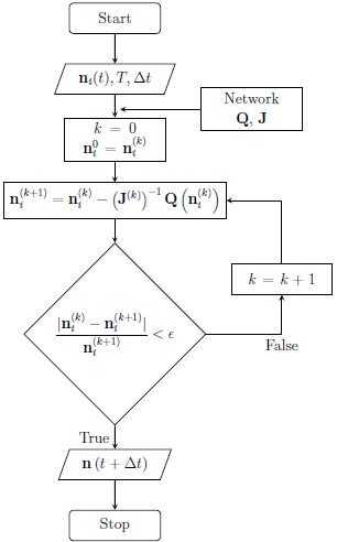
Fig. 1 KIMYA flow chart. Our code receives the initial densities of each species, the gas temperature and an arbitrary time-step and returns the time-advanced densities.
We have developed a benchmark suite using the network that will be described in § 5.3, with eleven chemical species and 40 chemical reactions. As we will see later, this particular benchmark will serve to check the operation of the code when compared to laboratory experiments. We have run a benchmark test for 104, 105 and 106 timesteps. Our code solves a single timestep in ≈ 3.9 × 10⁻⁵ seconds of wall-clock time. This feature is relevant when one wants to couple this solver with a multi-dimensional gasdynamic code, where one should find the solution for each species in each of the 104 −109 cells at every timestep.
4. THE REACTIVE FLOW EQUATIONS
KIMYA is designed for inclusion in reactive flow numerical codes. Hydrodynamic codes in one, two or three dimensions solve the gas dynamic (or magnetohydrodynamic) equations in a discretized space. In the discrete “cells”, the mass, momentum, energy conservation equations are solved together with the chemical network (to which one adds advection terms for each species). Usually, in a complete simulation there are typically from 105 to 109 cells, and each one is advanced in time for thousands of timesteps, so that a fast integrator for the chemical network is clearly essential.
The gasdynamic equations are:
where ρ, u and P are the gas density, velocity and pressure, respectively. γ is the specific heat ratio. G and L are the thermal energy gain and loss (respectively) due to interaction with the radiative field or to gains/losses associated with the latent heat of the chemical reactions and/or the internal energy of the molecular/atomic/ionic species. The thermal pressure is given by
where n is the total density (of molecules+atoms+ions) and ne is the electron density.
The complete set of equations for a reactive flow can then be written for a 2D flow as:
where n1, n2,. . . , nN are the densities of the different species. The vector U contains the so-called conservative variables. ρ, T y P, were defined previously, u and υ are the velocity in the x and y direction (respectively), and E is the energy written as:
The thermal pressure P is given by equation 17.
We note that the evolution equations of the chemical network were included as N continuity equations (as active scalars) and the sources Si are given by the right hand side of equation 2. These source terms should also include the appropriate geometrical terms when considering 2D, axisymmetric flow problems. Solutions to this set of equations are presented below.
5. NUMERICAL AND EXPERIMENTAL MODELS TO CODE VERIFICATION
In order to show the characteristics of the KIMYA astrochemical code we developed three numerical simulations. We first try a standard test presented by Braun, Herron & Kahaner (1988), who used the ACUCHEMc1ode. The second test is a dark cloud model, which we describe in § 5.2. Our third test consists of a calculation of the nitric oxide formation with a laser induced plasma (meant to model a lightning discharge), which is described in § 5.3. In all cases, the maximum number of iterations mentioned in § 2.1 is Nit = 40. In all cases the code reaches the convergence criterion after a smaller number of iterations.
5.1. Sequence Reactions Test
In this section, we show the implementation of the KIMYA code for two reaction systems proposed by Braun, Herron & Kahaner (1988): a sequence and a reverse reaction system.
The first test is the system of sequence reactions:
where, a, b, c and d are the species. The total density is:
The creation and destruction rates of the species are given by:
and one can calculate the density of species d from the conservation equation (24).
We rewrite equations (24)-(25) in the form of equation (5):
The root of this set of equations then gives the time-advanced solution.
With equations (26), we can calculate the Jacobian matrix,
Then, using the set of equations (26) and the Jacobian matrix (equation 27) in equation (8) we carry out a time integration from t = 0 to t = 20. For the convergence factor (see equation 10) we set β = 0.0 (i.e., f = 1), and we chose an ϵ = 10−5 tolerance. We consider initial densities na = 1 and nb = nc = nd = 0 (in dimensionless units).
Figure 2 shows the densities of the species a, b, c and d as functions of time (in dimensionless units); the solid, dotted, dashed and dot-dashed lines, denote the na , nb , nc and nd densities, respectively and the diamonds the values calculated using the standard ACUCHEM code. The values obtained with our code are in very good agreement with the results obtained using ACUCHEM.

Fig. 2 Densities of species a, b, c and d as a function of time (in dimensionless units) obtained from the sequence test (see equations 24-25). The solid, dotted, dashed and dot-dashed lines, represent the na , nb , nc and nd densities obtained with KIMYA, respectively, and the diamonds the corresponding values obtained using ACUCHEM.
5.2. Dark Cloud Model
Dark clouds consist of cold (≈ 10 K), dense (103 − 106) cm3, and dark regions (opaque to visible and UV radiation) which are composed mainly of gas-phase molecular material. The dark clouds are very inhomogeneous, and usually present dense, filamentary structures. Also, the dust present in these condensations completely absorbs the photons of optical and UV wavelengths.
Following the work of McElroy et al. (2013), we consider an isotropic and homogeneous medium with n(H2)=104 cm−3, and T =10 K. We want to compare the chemical concentrations obtained by McElroy et al. (2013), who used the complete network of the umist database that includes direct cosmic-ray ionization reactions, cosmic-ray-induced photoreactions and interstellar photoreactions, in the case of tmc-1. This complete network is composed of 467 species and 6174 reactions. We have chosen a reduced subset of species and reactions (13 species with 146 reactions, see below) that correctly reproduces the chemical evolution, but allows a significantly faster time-integration. We are mostly interested in reproducing the density of OH, CO, H2O and H2, which are some of the most important molecules in the ISM, and which dominate the molecular cooling function (see Neufeld et al. 1993, 1995).
In order to compute our (simplified) dark cloud model, we use the following selection criteria for the reactions:
the only ionized species are those that are formed solely of hydrogen;
the atoms taking part in the network are only H, C, and O;
the molecules contain at most three atoms;
the only grain-surface reaction included is the formation of H2 due to the combination of two atoms of H:
where n H and n HI are the total number of H nuclei and the density of neutral atomic hydrogen, respectively.
Taking into account these considerations, we obtain a network with 13 species (H, H+, CH, CH2, H2O, OH, CO, C, C2, O, O2, HCO, CO2) together with 146 reactions (including the formation in dust of H2). We must note that, according to these criteria, direct cosmic-ray ionization reactions, cosmicray-induced photoreactions and interstellar photoreactions are excluded. The reaction coefficients are set to zero outside the temperature range in which they are valid.
We show the initial conditions for the dark cloud model in Table 1. The only molecule that has a nonzero concentration at the beginning of the simulation is H2.
Table 1 Initial conditions in KIMYA.
| Species i | ni /nH1 | Species i | ni /nH |
|---|---|---|---|
| H2 | 0.5 | H | 5.0(-5) |
| C | 1.4(-4) | O | 3.2(-4) |
1nH is yhe number density of H nuclei.
The a(b) = a × 10b format has been used.
We ran our simulation for 108 yr. The results obtained are shown in Columns 2 and 5 of Table 2. Columns 3 and 6 give the values taken from the webpage of the umist database with rate 12 (McElroy et al. 2013) evolved up to the same time as our KIMYA simulation.
Table 2 Densities relative to H2.*
| Species | Density log (X/H2) | Species | Density log (X/H2) | ||
|---|---|---|---|---|---|
| Rate12 | KIMYA | Rate12 | KIMYA | ||
| H | -3.60 | -3.60 | C | -4.42 | -8.43 |
| H+ | -4.91 | -10.02 | C2 | -17.00 | -12.43 |
| CH | -9.96 | -10.47 | O | -3.55 | -3.54 |
| CH2 | -3.95 | -11.33 | O2 | -4.03 | -4.19 |
| H2O | -4.33 | -6.35 | HCO | -17.00 | -11.25 |
| OH | -7.93 | -7.49 | CO2 | -7.08 | -6.94 |
| CO | -3.88 | -3.55 | |||
*In a dark cloud model after 108 years.
We observe that the final concentrations of species like H, O, OH, CO, CH, and CO2 are very similar to those reported in the umist homepage. This fact is important if we consider that these molecules are some of the most important for comparisons with astrochemical models and observations, since they are the most abundant in the ISM and play an important role in calculating the molecular cooling. Also, this first analysis will serve as a basis to explore and study in more detail what kind of reactions are needed in order to improve the chemical evolution of the different species.
5.3. Nitric Oxide Formed During Lightning Discharge
The production mechanism of nitrogen oxides by electrical discharges has been discussed by several authors, starting with the paper of Stark et al. (1996). The velocity of the shock fronts generated by laboratory scale discharges has been measured, and was found to be too slow to raise the air temperature to the ≈ 3000 K necessary for nitrogen fixation by the Zel’dovich mechanism (Zel’dovich & Raizer, 1966). The freeze out mixing ratio of NOx in air has been measured directly for low pressure discharges and was found to be of the order expected from the Zel’dovich mechanism for gas cooling over a timescale far longer than the duration of the shock front.
Navarro-González, McKay & Mvondo (2001a) presented an experimental study of the formation of nitric oxide (NO) during a lightning discharge. Lightning was simulated in the laboratory by a plasma generated with a pulsed Nd-YAG laser. They presented the experimental variation of the nitric oxide yield as a function of the CO2 mixing ratio in simulated lightning in primitive atmospheres. The atmospheres are composed of CO2 and N2 at 1 bar, and all samples were irradiated at 20ºC from 5 to 30 min.
Navarro-González et al. (2001b) reported an experimental assessment of the contributions of the shock wave and the hot plasma bubble to the production of nitric oxide by simulated lightning. Their results provided a picture of the temperature evolution of a simulated lightning discharge from nanosecond to millisecond time scales, and quantitatively assessed the contributions of the shock wave and the bubble to the nitrogen fixation rate by simulated lightning.
The experimental setup consisted of a pulsing Nd:YAG laser which was focussed within an enclosure with gas of the chosen initial chemical composition. In the focal region, an approximately conically shaped plasma bubble was produced in each pulse, and this plasma bubble subsequently expanded producing a central, hot gas region and an outwards moving shock. After a large number of laser pulses, the chemical composition of the enclosed gas was analyzed (see, e.g., Navarro-González, McKay & Mvondo 2001a). We then modeled this flow configuration by studying the time-evolution of hot, initially conical bubbles that expand into an initially homogeneous environment.
In order to study the formation of NO in these experiments, we applied KIMYA in two different ways: as a zero-dimensional model using the techniques shown in § 2 (using the experimentally determined time-evolution of the plasma/hot air and shock wave temperatures), and a gasdynamic model using the reactive flow equations described in § 4.
5.3.1. Zero-Dimensional Model
We first compute “0D” numerical simulations (i.e., single parcel models) of NO formation using a gas with atmospheric pressure and an initial temperature of 300 K. We used a gas that was initially composed only of CO2 and N2. We then performed a set of numerical simulations changing the initial chemical composition of the gas, that is, changing the proportion of CO2 in the initial gas density (
We used the temporal evolution of the temperature for the hot air bubble and the shock wave obtained experimentally by Navarro-González, McKay & Mvondo (2001a). These temperature time-evolutions are shown in Figure 3. We performed numerical integrations using these two temperature profiles, for 3000 consecutive pulses with a frequency of 1 Hz (one pulse per second).

Fig. 3 Temporal evolution of the shock wave temperature (top) and the plasma/hot air temperature (bottom) obtained from a laser induced plasma with a 300 mJ per pulse discharge energy (see also Navarro-González et al. 2001b). The diamonds represent the experimental data, the solid line the fitted curve used to run the numerical models.
The simulations include a chemical network of 11 species and 40 reactions. The reactions and the coefficients α and γ in the Arrhenius equation (k = αeγ/RT, where T is the gas temperature) are shown in Table 3, Columns 2, 3 and 4, respectively.
Table 3 gas phase reactions used to model the no formed during lightning discharge.
| No. | Reaction | α | γ[kJ] |
|---|---|---|---|
| 1 | N + N + M → N2 + M | 2.6 × 10⁻³³ | -3.7 |
| 2 | N + O +M → NO + M | 2.6 × 10⁻³³ | -3.1 |
| 3 | N2 + M → N + N +M | 8.5 × 10⁻⁴ | 1102.2 |
| 4 | N2 + e → N + N + e | 8.1 × 10⁻¹³ | 0. |
| 5 | NO + M → N + O + M | 3.1 × 10⁻⁹ | 628.5 |
| 6 | NO + N → N2 + O | 3.2 × 10⁻¹¹ | 1.4 |
| 7 | NO + O → N + O2 | 1.2 × 10⁻¹¹ | 169.7 |
| 8 | NO + O + M → NO2 + M | 7.0 × 10⁻³³ | -5.7 |
| 9 | NO + NO + O2 → NO2 + NO2 | 3.3 × 10-39 | -4.4 |
| 10 | NO + O2 + M → NO3 + M | 5.7 × 10-41 | 1.8 |
| 11 | NO + NO → N2 + O2 | 2.5 × 10⁻¹¹ | 254.9 |
| 12 | NO + NO → N2O + O | 4.5 × 10⁻¹² | 267.7 |
| 13 | NO + O3 → NO2 + O2 | 2.3 × 10⁻¹² | 11.7 |
| 14 | NO2 + M → NO + O + M | 1.2 × 10⁻¹² | 117.3 |
| 15 | NO2 + O → NO + O2 | 5.8 × 10⁻¹² | 0.7 |
| 16 | NO2 + O + M → NO3 + M | 1.7 × 10⁻³³ | -8.7 |
| 17 | NO2 + N → N2O + O | 5.8 × 10⁻¹² | -1.8 |
| 18 | NO2 + O3 → NO3 + O2 | 3.2 × 10⁻¹³ | 22.1 |
| 19 | NO2 + NO2 → NO + NO + O2 | 2.7 × 10⁻¹² | 109.3 |
| 20 | NO2 + NO2 → NO3 + NO | 5.7 × 10⁻¹² | 96.4 |
| 21 | NO3 + M → NO + O2 + M | 4.5 × 10⁻¹³ | 17.6 |
| 22 | NO3 + O → NO2 + O2 | 1.0 × 10⁻¹¹ | 0. |
| 23 | NO3 + NO → NO2 + NO2 | 4.8 × 10⁻¹² | -3. 6 |
| 24 | NO3 + NO2 → NO + NO2 + O2 | 1.5 × 10⁻¹³ | 13.3 |
| 25 | N2O + M → N2 + O + M | 3.5 × 10⁻¹⁰ | 220.6 |
| 26 | N2O + O → N2 + O2 | 2.6 × 10⁻¹⁰ | 118.8 |
| 27 | N2O + O → NO + NO | 1.4 × 10⁻¹⁰ | 114.4 |
| 28 | N2O + NO → N2 + NO2 | 3.6 × 10⁻¹⁰ | 211.5 |
| 29 | O + O M → O2 + M | 1.7 × 10⁻³⁴ | -6.0 |
| 30 | O + O2 + M → O3 + M | 9.2 × 10⁻³⁵ | -4.3 |
| 31 | O2 + M → O + O + M | 5.0 × 10⁻⁷ | 493.0 |
| 33 | O2 + e → O + O + e | 4.3 × 10⁻¹¹ | 0. |
| 34 | O2 + N → NO + O | 1.5 × 10⁻¹⁰ | 63.1 |
| 34 | O3 + M → O2 + O + M | 1.2 × 10⁻⁹ | 95.5 |
| 35 | O3 + O → O2 + O2 | 1.2 × 10⁻¹¹ | 17.6 |
| 36 | O3 + N → NO + O2 | 5.7 × 10⁻¹³ | 0. |
| 37 | CO2 → CO + O | 1.3 × 10⁻⁹ | -424 |
| 38 | CO + O → CO2 | 1.7 × 10⁻³³ | -12.5 |
| 39 | CO2 + N → NO + CO | 3.2 × 10⁻¹³ | -1710. |
| 40 | O + CO2 → O2 + CO | 2.46 × 10⁻¹¹ | -220. |
Figure 4 shows the number of molecules of nitric oxide formed by the laser pulse per unit energy (of the laser) versus the initial concentration of CO2. The dash-dotted and dashed lines are the final concentrations (after the 3000 pulses, see above) obtained for the plasma/hot air bubble (dash-dotted line) and for the shock wave (dashed line), and the diamond symbols are the experimental measurements (with their errors) for all of the gas (bubble+shock wave) presented by Navarro-González, McKay & Mvondo (2001a).

Fig. 4 The variation of the nitric oxide yield as a function of the CO2 mixing ratio in simulated lightning for the experimental data (diamonds) and the three numerical models. The dash-dotted (plasma/hot air bubble) and dashed lines (shock wave) correspond to the zero-dimensional model. The solid line corresponds to the hydrodinamical model.
It is clear that for
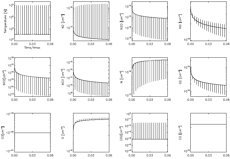
Figure 5 shows the evolution of the plasma temperature and numerical densities of N, N2, N2O, NO, NO2, NO3, O, O2, O3, CO and CO2 for the first 18 simulated pulses. The peaks in the plasma temperature correspond to the energy injection times (i.e., to the laser pulses, which are assumed to produce instantaneous temperature rises). The concentrations of N2, NO, O and CO2 increase and the concentrations of N, N2 O, NO, NO2, NO3 and O2 decrease in the pulses. The NO yield has a peak in each pulse, but after ≈ 1200 pulses it attains an almost timeindependent, constant value. This is the value that is compared with the experimental measurements.
5.3.2. Gasdynamic Model
We computed reactive flow simulations using the walixce 2D code (Esquivel et al. 2010) + KIMYA. The walixce 2D code solves the gas dynamic equations (see equations 14-16 in § 4) in a cylindrical, two-dimensional adaptive mesh, using a second order HLLC Riemann solver (Toro et al. 1994). This fusion of the two codes is named WALKIMYA 2d. To carry out the numerical simulations, we then integrate the gasdynamic equations and continuity/reaction rate equations for all species, as discussed previously in § 4.
The adaptative mesh consist of four root blocks of 16 × 16 cells, with 7 levels of refinement, yielding a maximum resolution of 4096 × 1024 (axial × radial) cells. The maximum resolution (along the two axes) is of 1.95 × 10⁻³ cm. The boundary conditions used are reflection on the symmetry axis and transmission everywhere else. The size of the mesh is large enough so that the choice of outer boundaries does not affect the simulation.
The timestep is chosen with the traditional CFL (Courant-Friedrichs-Lewy) stability condition of the explicit gasdynamic integrator of the walixce 2D code (Esquivel et al. 2010). The same timestep is used for the (simultaneous) integration of the chemical reaction terms with the KIMYA routines.
The numerical simulations are initialized with an environment of atmospheric pressure and a temperature of 300 K. A γ = 7/5, constant specific heat ratio is assumed. The hot plasma bubble (generated in the experiment in the focal region of a focussed laser pulse) is introduced in the center of the computational mesh, as a hot, T0 ~ 104 K cone of 0.25 cm (axial) length and α = 30◦ half-opening angle (the initial density within the cone having the environmental value, and the values chosen for T0 are discussed below). This high pressure cone expands, driving a shock wave into the unperturbed environment. The simulations evolve until a time of 2.0 × 10⁻⁵ sec.
In order to reproduce the time-dependent evolution of the shock wave produced by an expanding, laser-generated plasma bubble, we computed simulations using initial temperatures (for the hot cone) T0 = 7000, 12000 and 24000 K. Figure 6 shows the average radius of the shock wave as a function of time, and we see that the three chosen values of T0 lead to results that lie close to the experimentally measured shock wave radius (see Raga et al. 2000, and references therein). The predictions of the chemical evolution that we present below are obtained from simulations with T0 = 12000 K.
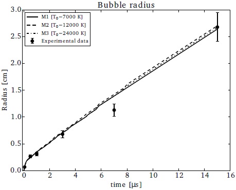
Fig. 6 Radius of the simulated bubble versus time using different initial temperatures for the hot cone: T0 = 7000, 12000 and 24000 K (solid, dashed and dotted line, respectively). The symbols represent the experimental data together with their respective errors.
Figure 7 shows density and temperature maps for two stages of the bubble evolution. The two panels on the left correspond to density maps for evolutionary times of 2×10⁻⁶ and 2×10⁻⁵ sec, and the two panels on the right side are the temperature maps at the same two evolutionary times. At 2×10⁻⁶ sec, the gas which is compressed by the shock wave and a low density, inner region (with a temperature ≈ 104 K) are clearly seen. At 10−5 sec, the shock wave is no longer visible, and the central, low density region has a ≈ 1000 K temperature.

Fig. 7 Density (left) and temperature maps (right) at t = 2 × 10⁻⁶ and 2×10⁻⁵ s (as indicated in the frames). In each panel, the left frames are the density maps and the right frames are the temperature maps.
The gas was initially composed only of CO2 and N2. We compute simulations changing the initial value of
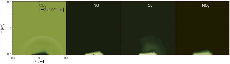
We then solved the evolutionary densities of 11 chemical species. Figure 8 shows the density maps of CO2, NO, O3 and NO2 (left, center-left, centerright and right panels, respectively) at 2×10⁻⁶ sec obtained from the simulation with
The total NO yields obtained from the simulations are shown as a solid line in Figure 4. It is clear that these yields are consistent with the experimental measurements of Navarro-González, McKay & Mvondo (2001a) over most of the explored
Finally, Figure 9 shows the total yield of all of the molecules included in the numerical simulations. We find that for initial CO2 densities larger than 0.865, N2O, NO2, NO3 and O3 do not form, but in environments richer in N2 the formation of these oxides is very important.

5.4. Scaling of the Computational Time
In order to illustrate the scaling of our reactive gasdynamic code as a function of the number of species and reactions, we have carried out a set of simulations similar to the ones of § 5.3.2. In these simulations we changed:
the number of reactions (models M2a, M2b, M2c, M2d and M2e), but keeping the same number of species,
the number of reactions and species (models M3, M4, M5 and M6).
The numbers of species and reactions used in these two sequences of simulations are given in Table 4.
Table 4 Numerical models.
| Model | Number of species | Number of reactions | Scaled time |
|---|---|---|---|
| M1 | 0a | 0 | 1.0 |
| M2a | 31 | 10 | 1.11 |
| M2b | 31 | 50 | 1.31 |
| M2c | 31 | 75 | 1.38 |
| M2d | 31 | 100 | 1.62 |
| M2e | 31 | 140 | 1.82 |
| M3 | 2 | 1 | 1.24 |
| M4 | 5 | 6 | 1.26 |
| M5 | 15 | 47 | 1.73 |
| M6 | 19 | 82 | 1.75 |
| M2e | 31 | 140 | 1.82 |
aSolving only the hydrodynamic equations.
In the left panel of Figure 10 (and also in Column 4 of Table 4), we show the scaled computational time as a function of number of reactions. We have scaled the computational times to the computational time of a purely hydrodynamic simulation (model M1, with no chemical species). From these models (models M2a, b, c, d and e) we see an approximately linear increase in computational time with number of chemical reactions (left panel of Figure 10). For the case of 140 reactions (model M2e), the computational time is ≈ 1.8 times larger than that of the purely gasdynamic simulation (model M1, see Table 4).

Fig. 10 Left panel: computational time vs. number of reactions for the M2a, M2b, M2c, M2d, M2e sequence (with constant number of species, see Table 4). Right panel: scaled computational time vs. number of species for the sequence of models M3, M4, M5, M6 and M2e, with increasing numbers of species and reactions (see Table 4).
For the sequence of models with increasing number of species and reactions (models M3, M4, M5, M6 and M2e, see Table 4) we obtain a rapid growth of computational time for up to 15 species, and a slower growth from 15 to 31 species (see the right panel of Figure 10).
6. DISCUSSION AND CONCLUSION
We have presented the new KIMYA numerical code for solving chemical reaction networks. This code was written in Fortran 90 and has subroutines and modules providing the tools to solve the kinetical chemistry for a reaction network chosen by the user.
In order to solve the system of ODEs, we implemented an implicit numerical solver (based on the standard, Newton-Raphson method). This method in principle converges for arbitrary values of the chosen timestep.
We simulated two problems of interest:
a dark cloud model; we computed a single-parcel model which we compare with the previous work of McElroy et al. (2013). We find good agreement, especially for species like O, OH, H2O, CO, and CO2. The chemical network used for our simulation consists of 13 species: H, H+, CH, CH2, H2O, OH, CO, C, C2, O, O2, HCO, CO2, and 146 reactions;
laser laboratory experiments of the formation of nitric oxide during lightning discharges: we computed single-parcel models and axisymmetric reactive gasdynamic simulations, and we compared the induced chemistry with the experimental study of NO formation presented in Navarro-González, McKay & Mvondo (2001a). We computed models changing the initial chemical composition of the gas, and obtained the chemical composition after a single laser pulse and after 3000 pulses. We found that for initial CO2 concentrations in the 0.2 <
Though this second problem has no direct astrophysical application, it allows us to evaluate the precision of a reactive gasdynamic simulation, by comparing the final (spatially integrated) chemical composition obtained from the simulation with laboratory measurements. This kind of test should be attempted with different astrophysical codes to evaluate whether or not the computed chemistry converges to the appropriate solution.
We found that for a benchmark suite solving 11 chemical species and 40 chemical reactions, our code solves a single timestep in ≈ 3.9 × 10⁻⁵ s. We found that the speed of our algorithm is sufficient for combining it with a multi-dimensional gasdynamic (or magnetohydrodynamic) code, in which the chemical evolution must be solved in 104 − 109 computational cells.
The KIMYA code is efficient and can handle a complex set of chemical reactions that can be used in studies of interstellar chemistry, planetary atmospheres, combustion and detonation experiments, and air pollution, among others.
KIMYA can be used to solve a chemical reaction network for a “single parcel” model. Also, the code can be integrated in a full gasdynamic (or magnetohydrodynamic) simulation, computing the temporal evolution of the chemical species. The simplest possible implicit timestep (see § 2) carried out by KIMYA gives a short computational time which results in only moderate (≈ factor of 2, see § 5.4) increases over “non-reactive” hydrodynamic simulations (without a chemical network).
Although the main utility of the code is to model different phenomena in the ISM, it can also be used in other areas (see above). We found that comparisons between the numerical simulations and experiments (see § 5) show good agreement. As far as we are aware, this is the first time that an astrophysical reactive gasdynamic code has been tested with laboratory experiments. This test gives us confidence that our code is working correctly. Clearly, other reactive flow code developers could use the experimental results we have described here in order to test their codes.
As a future release, in order to make KIMYA more user friendly, we will include an automation of the chemical network generator. The code will then write the rate equations and the elements of the Jacobian matrix directly from the reactions chosen by the user. Also, we will develop procedures for defining the set of reactions, choosing the more representative reactions for a particular problem and limiting the number of species. This is not an easy task, and a substantial effort is being made to find the best way to do this, as discussed, e. g. by Wiebe, Semenov & Henning (2003) and Grassi et al. (2012) for the case of astrochemical networks.

