


 nova página do texto(beta)
 Inglês (pdf)
 Artigo em XML
 Referências do artigo
 Enviar este artigo por email
 Citado por SciELO
  Similares em
SciELO
Similares em
SciELO 
 Permalink
1. INTRODUCTION
Nowadays the κ distribution is the focus in the model of space plasmas (Hasegawa et al. 1985; Sabry et al. 2012; Saini and Kourakis 2008; Saini et al. 2009; Saini and Kourakis 2010). Note that for all velocities, the κ distribution function approaches the Maxwellian distribution (which is considered a special case) for very large κ (κ → ∞). Particles described by κ distribution are found in many kinds of plasma environments like the solar wind, the Earth’s magnetospheric plasma sheet, Jupiter, and Saturn (Abdelsalam 2013; El-Shewy et al. 2011; Hellberg and Mace 2002; Leubner 2004; Sabry et al. 2012).
The inclusion of superthermal particles in a plasma characterizes the high energy region in space, and the presence of superthermal particles causes velocity space diffusion (Hasegawa et al. 1985). Many authors used the kappa distribution to study superthermal particles (ions, positrons, and electrons) (Abdelsalam et al. 2008; Ali et al. 2007; Pakzad 2011). A one-dimensional kappa distribution along a preferred direction in space and a Maxwellian distribution perpendicular to it were the focus of many studies (Hellberg and Mace 2002; Kourakis and Williams 2013). However, few works dealt with superthermal ions (as in Hellberg and Mace 2002; Saini and Kourakis 2008). Kappa distributions are more suitable to study the solar wind (Pierrard and Lemaire 1996), Jupiter and Saturn (Krimigis et al. 1983) or to explain spacecraft data in the Earth’s magnetospheric plasma sheet (Christon et al. 1988) and the velocity filtration effect in the solar corona (Pierrard and Lemaire 1996).
Schippers et al. (2008) analyzed the CAPS/ELS and MIMI/ LEMMS data from the Cassini spacecraft orbiting Saturn over a range of 5.420 Rs, where Rs ≈ 60300 km is the radius of Saturn (Alam et al. 2013). For Saturn’s F-ring the nonlinear structure could be due to solitons for a very short range of plasma parameters and the largest possible solitary waves generated in plasma system with kappa-distribution with a specific velocity distribution are found to be smaller than those found in a Maxwell-Boltzmann plasma (Pakzad 2011; Saini et al. 2009; Shukla and Silin 1992). Recently, DAWs became interesting for nonlinear waves because dust particles are found in interstellar clouds (Abdelsalam 2013; El-Shewy et al. 2011; Leubner 2004; Moslem et al. 2010; Sabry et al. 2012; Shukla and Silin 1992). Depending on the nature of the charge and mass density of the dust grains, it is possible to calculate the phase velocity and the corresponding frequency for any wave as well as for a plasma system.
Here, we consider a simple model discussed in § 2 to study the effective superthermal phenomena for both electrons and ions in astrophysical compact objects and space. First, we derive the Sagdeev potential to study the large amplitude wave structure in § 3. We also derive the KdV equation with its solution for solitary nonlinear waves using a reductive perturbation method as discussed in § 4. Finally an extended homogeneous balance method is used to solve the KdV equation (Abdelsalam et al. 2008; Abdelsalam 2010; Pakzad 2011) in § 5. The numerical analysis is presented in § 6. The conclusion is summarized in § 7.
2. BASIC EQUATIONS
We considered a plasma system containing both superthermal electrons and ions with a kappa distribution, and heavy dust particles positively charged, i.e., our plasma model is composed of dust, superthermal ions and electrons. The nonlinear propagation of the electrostatic DAWs is described by
where the ions and electrons obey the κ distribution law (Pakzad 2011) as follows:
and
where κ is a real parameter measuring the deviation of the potential energy from the Boltzmann distribution. In the limit κ → ∞, the superthermal distribution reduces to the Boltzmann distribution.
In the last equations, nj is the number density (where j = i,d,e), ud is the dust fluid velocity, ϕ is the electrostatic potential, and σ = Te /Ti is the unperturbed electron-to-ion temperature ratio. At equilibrium, we have μd + μi = 1, where μd = nd0 /ne0, μi = ni0/ne0, and nd0 is the unperturbed dust number density (Abdelsalam et al. 2008).
3. LARGE AMPLITUDE OF THE SAGDEEV-LIKE POTENTIAL AND NUMERICAL ANALYSIS
First, we derive a Sagdeev-type pseudo-potential as an energy balance-like equation (Abdelsalam 2010) and then we numerically solve the equation to study the properties of both the Sagdeev-like potential and a solitary pulse.
To study the finite amplitude DASWs and their properties, we assume that the dependent
variables in equations (1)-(5) depend on one variable η =
x−Mt, where M is the Mach
number (soliton velocity/Csd) and
η has been normalized by
λD. Thus, we obtain from
equations (1) and (2) that
where the Sagdeev potential for our purposes reads
Equation (7) can be regarded as an ‘energy integral’ of an oscillating particle of unit mass, with a velocity dϕ/dη and position ϕ in a potential V(ϕ).
If the DASWs exist, then the Sagdeev potential needs to satisfy the following conditions: (a)
at ϕ = 0, d2
V/dϕ2 < 0; (b) we can find a
critical value (max. or min. value of ϕ)
ϕm, at which
V(ϕm) = 0; and
(c), when V(ϕ) < 0 then we find 0 <
ϕ < ϕm. So we
can obtain the maximum and minimum values of the Mach number M for
which solitons exist. Using the condition (a), the lower limit of Mach number
M is
The latter inequality provides the maximum M, which turns out to depend on the parameters μi and σ. Therefore, the following inequality can help us to calculate the Mach number range
We obtain the range of Mach number as 0.45 < M < 1.2 for the values of μ i = 0.25 and σ = 0.9. The existence of supersonic and subsonic solitons is noted. By increasing the ratio μi, to μi = 0.4, the Mach number range reads 0.45 < M < 0.99, which shows that the increase of μi leads to an expansion of subsonic solitons.
In Figures 1 and 2, the Sagdeev potential in equation (8) has been numerically analyzed. Note that the profile of the potential depends on α and M. Figure 1 shows the effect of the ion-to-electron number density ratio μi on the compressive solitary pulse for subsonic and supersonic waves. An increase of μi (which means a decrease of μd) makes the potential deeper and wider. However, a supersonic soliton has deeper amplitude and wider depth than a subsonic soliton.
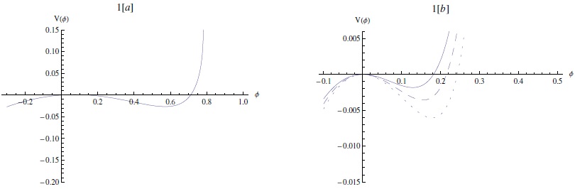
Fig. 1 The Sagdeev potential V(ϕ) [represented by equation (7)] against the potential ϕ. (a) supersonic solitary pulse for M = 1.1. (b) subsonic solitary pulse for M = 0.8. The effect of varying μi = 0.2 (solid curve), μi = 0.3 (dashed curve), and μi = 0.4 (dotted curve), where σ = 0.9 is shown. The color figure can be viewed online.
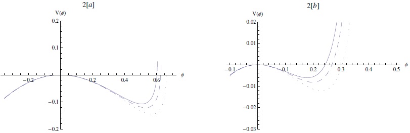
Fig. 2 The Sagdeev potential V(ϕ) [represented by equation (7)] against the potential ϕ. (a) supersonic solitary pulse for M = 1.1 (solid curve), M = 1.15 (dashed curve), and M = 1.2 (dotted curve). (b) subsonic solitary pulse for M = 0.8 (solid curve), M = 0.85 (dashed curve), and M = 0.9 (dotted curve). Here, μi = 0.3 and σ = 0.95. The color figure can be viewed online.
Figure 2 shows that increasing the Mach number (M) leads to the expansion of the permitted region of the potential values associated with the localized excitations, which implies that faster pulse excitations will be large and narrow. The energy in equation (6) has been numerically solved for many parameters. The profiles of the potential pulse are drawn in Figure 3. It is found that shorter pulses are wider than longer pulses and that increasing M causes an increase in the amplitude and a decrease in the width.
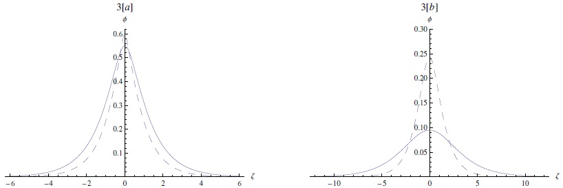
Fig. 3 The potential ϕ [the solution of equation (6)] is depicted against ζ. (a) supersonic solitary pulse for M = 1.1 (solid curve) and M = 1.25 (dashed curve). (b) subsonic solitary pulse for M = 0.8 (solid curve) and M = 0.9 (dashed curve). Here μi = 0.2 and σ = 0.8. The color figure can be viewed online.
4. KORTEWEG-DE VRIES EQUATION AND SOLUTION FOR NUMERICAL ANALYSIS
In this section, we study solitary waves with small and finite amplitude deriving the Korteweg-de Vries (KdV) equation using a nonlinear perturbation method to study dust-acoustic-solitary-waves (DASWs) (Abdelsalam 2010).
For the reductive perturbation method, we should use the stretched space-time coordinates ξ = ε1/2(x−ϑt) and τ = ε3/2t (Washimi and Tanituri 1966), where ϑ is the phase speed and ε is the smallness parameter measuring the weakness of the dispersion (0<ε<1). The dependent variables are expanded as
where n = 0,1,2,3,. . .,
and
Using the last stretching and expansions into equations (1)-(5), we isolate distinct orders in ϵ and derive the corresponding variable contributions. The lowest-order equations in ϵ read
and
Note that the minimum Mach number is identically ϑ.
The next order in ϵ yields the values for
where A is the nonlinear coefficient and B is the dispersion coefficient, respectively,
5. EXTENDED HOMOGENEOUS BALANCE METHOD TO SOLVE THE KDV EQUATION
The extended homogeneous balance (HB) method is applied to obtain many solutions for the KdV equation (Abdelsalam 2017; Abdel-Rady et al. 2010; El-Wakil et al. 2007; Wang 1995; Wang et al. 1995). Consider the KdV equation [equation (12)] as:
where α stands for A and β for B.
Applying the transformation u(ξ,τ) = U(η),η = ξ − λτ to equation (14), we find that U satisfies the following ordinary differential equation
Integrating (15) with respect to η once, we get
Now, balancing U 2 with U′′ gives the magnitude, |m| = 2. Hence, the solution should be of the form
where the Riccati equation is, ω′ = k + M ω + P ω2; here, ω is the angular frequency, ω′ = dω/d/ξ, k is the wave number, and M and P are the coefficient parameters; k and P cannot be zero (0).
Substituting the last equation equation (17) in equation (16), we get a polynomial equation ω. Now, equating the coefficient of ωi (i = 0, 1, 2, ...) to zero, we get a system of algebraic equations and by solving this system using package MATHEMATICA (Abdelsalam 2017), we obtain:
the first set:
the second set:
Four cases regarding the Riccati equation were previously published by Abdelsalam (2017). As full details of these four cases are already published, here they are not discussed. Case I is considered when P = 1 and M = 0. The Riccati equation gives two solutions for k < 0 and k > 0 separately. Case II is considered for balancing between ω′ and ω 2. An arbitrary constant, r = 1, is used for Case III. Finally, balancing ω′ with ω2 leads to |m| = 1, and Case IV is introduced. We will use the case numbers in this work to explain our current study. At this stage, we encourage the readers to consult Abdelsalam (2017).
For the first set of equations (18), if M = 0, P = 1 the obtained solutions will satisfy Case I of the solutions for the Riccati equation (Abdelsalam 2017). For k > 0, the solutions of the KdV equation of the type of equation (14), will be
For k < 0,
For k = 0,
Now with the compatibility condition, we obtain the solutions satisfying Cases II, III, and IV,
Therefore, substituting for P and k, from (18) into (25), and solving for p1, we find that
Hence, for Case II, we get the following solutions:
and
For Case III, the solution is
with the condition that p1 = 1. Finally, for Case IV,
with the condition that p1 = 1, and
with the condition that p1 = 2.
For the second set we are left only with solutions satisfying Cases II, III, and IV. Since the main criteria for these cases to be applicable is the compatibility condition,
from (19), it is found that
Therefore, solutions to equations of the type of equation (14) will be
and
For Case III,
where p1 = 1.
Finally for case IV,
with p1 = 1 and
with the condition that p1 = 2.
To investigate the nonlinear properties of solitary waves [as represented by equation (22)], for k = −ϑ/4β we express the solution equation (14) in the following form
where the amplitude is ϕ0 = 3u0/A and the width is ∆ = (4B/u0)1/2 for the solitary wave profiles caused by the balance between nonlinearity and dispersion. As the standard result for KdV we see that ϕ0∆2 = 12B/A = constant (for given ϑ) (Killian 2006).
6. NUMERICAL ANALYSIS
The extended HB is applied to give the traveling wave solutions for the KdV equation (Abdelsalam 2017; El-Wakil et al. 2007; Wang 1995). The obtained solutions cover many types of periodical, rational, singular and solitary wave solutions. As an example, the solution of equation (20) is a sinusoidal-type periodical solution shown in Figure 4. The solutions for equation (24) are of rational-type and the solution of equation (22) is a kink-type solitary wave solution. Note here that equations (23) and (31) are explosive/blowup solutions as depicted in Figure 5. The solution of equation (6) represents a soliton wave with amplitude ϕ0.
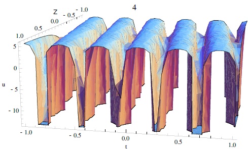
Fig. 4 3D plots of the solution of equation (20) with A = 0.5 and B = 2.9. The color figure can be viewed online.
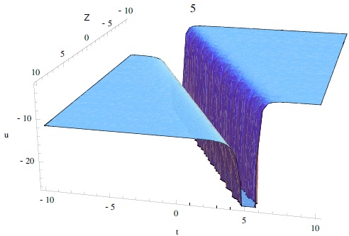
Fig. 5 3D plots of the solution equation (30) with A = 0.5, B = 2.9 and M = 0.9. The color figure can be viewed online.
Note that increasing the electron-to-ion temperature ratio σ = Te/Ti as well as the parameter κ will decrease the amplitude (as in Figure 6), while we can see in Figure 7 the effect of increasing the ion-to-electron number density ratio μi (which means a decrease of μd) which will make the soliton taller and wider. We can now compare this analytical solution to the numerical solution (obtained by numerical integration) of equation (6), in Figure 8. Note that the difference between the approximate and exact solutions increases with increasing nonlinearity, thus enhancing the amplitudes of pulses.
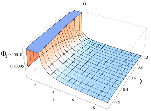
Fig. 6 The variation of the solitary pulse amplitude ϕ0 [equation (39)] against κ and σ for fixed values of μi = 0.22, and ϑ = 0.1. The color figure can be viewed online.
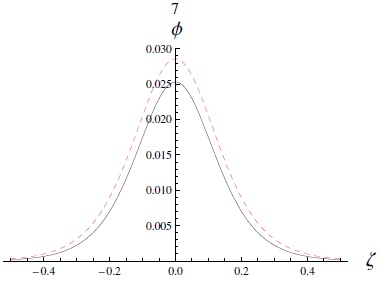
Fig. 7 The solitary potential excitation [as given by equation (39)] for varying the value of phase speed μi = 0.21 (solid curve) and μi = 0.3 (dashed curve) with κ = 3, σ = 0.9, and ϑ = 0.1. The color figure can be viewed online.
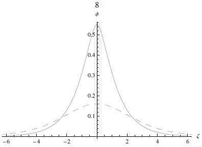
Fig. 8 The potential ϕ [exact/numerical integration of equation (7)] and the approximate potential [represented by equation (39)] are depicted against ζ. The solid and dashed curves represent the exact and approximate solutions, respectively. Here μi = 0.2, σ = 0.9, κ = 3, M = 1.1, and ϑ = 0.1. The color figure can be viewed online.
Overall, in this paper the nonlinear dust-acoustic solitary wave propagation is studied in a superthermal ionelectron-dust plasma. The dust is described by the hydrodynamic equations with superthermal electrons and ions. The Sagdeev equation is derived. It is shown that for low values of μi we can observe both supersonic and subsonic DAWs. While increasing μi leads to an expansion of subsonic solitons only, we discussed the reliance of the potential pulse excitation characteristics and of the pseudo-potential profiles on μi and the Mach number. The effects of the physical parameters have been studied on the localized DAWs structures/excitations and the propagating nonlinear structures. The extended homogeneous balance method extracts a wide range of solution structures using the techniques for solving partial differential equation (PDEs); the method is applied to the KdV equation. Many traveling wave solutions are formally derived for these equations, some of them new and interesting (Abdelsalam et al. 2008; Abdelsalam 2010, 2017; El-Wakil et al. 2007; Pakzad 2011; Wang et al. 1995). These solutions include many types of wave solutions.
7. CONCLUSION
In the previous investigations, it was confirmed that theoretically dust particles with positive charges are present in the outer magnetosphere of Jupiter and Saturn (Horanyi et al. 2004; Scarf 1969); the same speed for ions and electrons was considered to study the solitons and shock waves (Saleem et al. 2012). However, the existence of rogue waves was also found when the solar wind interacts with Jupiter’s magnetosphere (Tolba et al. 2015, 2017; Abdelghany et al. 2016) in the presence of positively charged dust particles (Horanyi et al. 2004; Saleem et al. 2012). Thus, nonlinear waves are also present in Jupiter’s magnetosphere and due to the presence of ions and electrons, the streaming dust acoustic wave speed effect does not contribute to the dust dynamics (Horanyi et al. 2004; Scarf 1969; Saleem et al. 2012; Tolba et al. 2015, 2017; Abdelghany et al. 2016). Thus in this work, we consider positively charged dust particles in our superthermal plasma model and study both large and small amplitude nonlinear wave propagation using the reductive perturbation method.
This work is mainly relevant to nonlinear DASWs in superthermal electrons and ions following κ distribution in an unmagnetized collisionless plasma. The dissipation of solitary waves (solution of the KdV equation) in the presence of positively charged dust particles is also studied numerically with the extended homogeneous balance method used to solve the KdV equation. Because of the large range of σ(= Te /Ti), the Landau damping effect on dissipation is negligible, but the damping of solitary waves is mainly caused by the ion-dust collision and the kinematic viscosity (Nakamura and Sarma 2001). Thus if we consider a viscosity term in the model the nonlinear structure for shock waves can be studied(Lu et al. 2006; Nakamura et al. 1999; Pakzad 2011). Some studies considered positrons in the plasma model as super-dense electron-positron-ion plasmas which also can be found in some astrophysical environments (Abdelsalam et al. 2008; Ali et al. 2007; Pakzad 2011).

