


 nueva página del texto (beta)
 Inglés (pdf)
 Artículo en XML
 Referencias del artículo
 Enviar artículo por email
 Citado por SciELO
  Similares en
SciELO
Similares en
SciELO 
 Permalink
1. INTRODUCTION
The Herbig-Haro object HH 30 consists of a pair of jets from a young star in the Taurus star formation region at a distance of 140 pc (Kenyon et al. 1994). Hubble Space Telescope (HST) images display a nearly edge-on, flared, reflection nebula on both sides of an opaque circumstellar disk, with collimated jets emitted perpendicularly to the disk on both sides and nearly in the plane of the sky: the declination angle is approximately 80º with respect to the line of sight (Hartigan and Morse 2007). The HH 30 jets extend out to about 0.22 pc from the stellar source in each direction (Lopez et al. 1995), but here we are concerned with the first 0.003 pc of the brighter (northeastern) blueshifted jet near its launch site. Since the nearly edge-on disk effectively blocks the stellar light, the jet can be studied as it emerges from the accretion disk.
This investigation will compute surface brightness maps for the HH 30 jet near its launch site in the forbidden [O I], [N II], and [S II] doublets by post-processing gas dynamical simulations of densities and temperatures, using spectral line emission data from the astrophysical spectral synthesis package Cloudy (version 13.03, Ferland et al. 2013). We will then compare the simulated surface brightness in each line with HST observations of Hartigan and Morse (2007) and with multiple-ion magnetohydrodynamic simulations of Tesileanu et al. (2014).
On a logarithmic scale, our surface brightness simulations along the center of the jet are always within ±7.5% of the observational data for all three doublets, and fit the observational data more tightly than the simulations of Tesileanu et al. (2014). (However, it is important to note that the aim of these authors was quite different: they simulated a generic MHD jet with radiative cooling and spectral emission from multiple ionic species, and then compared their generic simulation with the observational data from HH 30 and RW Aurigae.) More importantly, the general trend of our simulated surface brightness in each doublet closely follows and is in excellent agreement with the observational patterns, validating our choices of initial jet and ambient densities and jet temperature and the number and sequencing of the jet pulses over the 35 year evolution of the jet near its launch site. In addition, we can simulate surface brightness all the way up to the circumstellar disk.
The main focus of the investigation is to establish initial jet parameters and the exact sequence of pulses launched from the stellar source/disk system to yield agreement with the HST observations.
Small changes in the parameters for our simulations (initial jet and ambient densities, jet temperature, jet velocity, jet width, and the sequencing of pulses) produce density, temperature, radiative cooling, and surface brightness results that are similar to those presented here. However, large changes in any of the simulation parameters produce jets which clearly differ from the HH 30 observations. Based on our numerical experimentation, we do not expect any degeneracies in the choice of simulation parameters.
2. NUMERICAL METHODS AND RADIATIVE COOLING
To simulate astrophysical jets, we apply the WENO (weighted essentially non-oscillatory) method (Shu 1999)-a modern high-order upwind method-to the equations of gas dynamics with atomic and molecular radiative cooling (see Ha et al. 2005, Gardner & Dwyer 2009, Gardner et al. 2016). The equations of gas dynamics with radiative cooling can be written as hyperbolic conservation laws for mass, momentum, and energy:
where ρ = mn is the density of the gas, m is the average mass of the gas atoms or molecules, n is the number density, ui is the velocity, ρui is the momentum density, P = nkB T is the pressure, T is the temperature, and E is the energy density of the gas. Indices i, j equal 1, 2, 3, and repeated indices are summed over. The pressure is computed from the other state variables by the equation of state:
where γ is the polytropic gas constant.
We use a “one fluid” approximation and assume that the gas is predominantly H above 8000 K,
with the standard admixture of the most abundant elements in the interstellar medium
(ISM); while below 8000 K, we assume the gas is predominantly H2, with
n(H)/n(H2)
≈ 0.01. We make the further approximation that γ equals
Radiative cooling (see Figure 1) of the gas is incorporated through the right-hand side −C(n, T) of the energy conservation equation (3), where
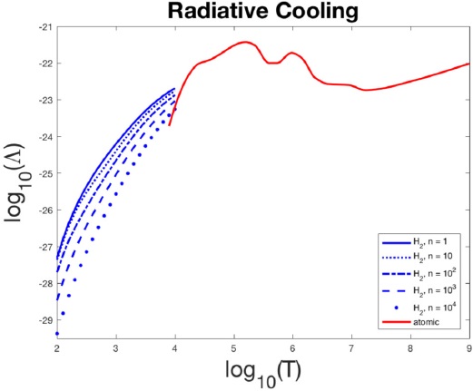
Fig. 1 Atomic Λ(T) and molecular Λ(n, T) = W (n, T)/n cooling functions: log10(Λ) with Λ in erg cm3 s−1, n in H atoms/cm3 (n = 100 corresponds to 50 H2 molecules/cm3), and T in K. The color figure can be viewed online.
with the model for Λ(T) taken from figure 8 of Schmutzler & Tscharnuter (1993) for atomic cooling, and the model for W(n,T) from figure 4 of Le Bourlot et al. (1999) for H2 molecular cooling. The atomic cooling model includes the relevant emission lines of the ten most abundant elements (H, He, C, N, O, Ne, Mg, Si, S, Fe) in the ISM, as well as relevant continuum processes.
We use a positivity preserving (Hu et al. 2013) version of the third-order WENO method (Shu 1999) for the gas dynamical simulations (Gardner et al. 2017). ENO and WENO schemes are high-order, upwind, finite-difference schemes devised for nonlinear hyperbolic conservation laws with piecewise smooth solutions containing sharp discontinuities like shock waves and contacts. Most numerical methods for gas dynamics can produce negative densities and pressures, breaking down in extreme circumstances involving very strong shock waves, shock waves impacting molecular clouds, strong vortex rollup, etc. By limiting the numerical flux, positivity preserving methods guarantee that the gas density and pressure always remain positive.
Below we calculate emission maps from the 2D cylindrically symmetric simulations of the HH 30 jet, at a distance of R = 140 pc. To calculate the [O I] (6300 + 6363Å), [N II] (6584 + 6548 Å), and [S II] (6716 + 6731Å) doublet emission, we post-processed the computed solutions using emissivities ϵ(n, T) extracted and tabulated from Cloudy, including an ionization fraction factor Xi (n,T) for the ions i of the different elements. In practice, we calculated a table of values for log10(ϵline) on a grid of (log10 (n), log10 (T)) values relevant in the simulations to each line, and then used bilinear interpolation in log10 (n) and log10 (T) to compute log10 (ϵline). For the simulations presented here, we calculated the emissivities for 2 ≤ log10(n) ≤ 8 with n in H atoms/cm3 with a spacing of 0.1 in log10(n); and for 3.8≤log10 (T) ≤6 with T in K with a spacing of 0.05 in log10(T).
Surface brightness Sline in any emission line was calculated by integrating along the line of sight through the jet and its surroundings
where R is the distance to the jet, and then converting to erg cm−2 arcsec−2 s−1.
In Gardner et al. (2016) , surface brightness maps from our gas dynamics/Cloudy simulations of the SVS 13 microjet-traced by the emission of the shock excited 1.644 μm [Fe II] line-and bow shock bubble-traced in the lower excitation 2.122 μm H2 line-projected onto the plane of the sky were shown to be in good qualitative agreement with (nonquantitative) observational images in these lines.
3. RESULTS OF NUMERICAL SIMULATIONS
Parallelized cylindrically symmetric simulations were performed on a 750∆z × 100∆r grid, spanning 1.5 × 1011 km by 0.4 × 1011 km (using the cylindrical symmetry), with each grid cell encompassing an effective Cartesian volume of (2 × 10⁸ km)3. The jet was emitted through a disk-shaped inflow region in the rz plane centered on the z-axis with a diameter of 109 km, and propagated along the z-axis with an initial velocity of 300 km s−1. The simulation parameters at t = 0 for the jet and ambient gas are given in Table 1. The jet is propagating into previous outflows, so although the far-field ambient is lighter than the jet, the immediate ambient near the stellar source is likely to be nearly as dense as the jet itself. Further, the tapering morphology of the HST observations of the jet imply that the jet density is near the ambient density: if the jet were much heavier than the ambient, the jet would create a strong bow shock and would itself be wider; if the jet were much lighter than the ambient, the jet would also create a strong bow shock, plus strong Kelvin-Helmholtz rollup and entrainment of the ambient gas. Note that the jet and ambient gas are not pressure matched.
Table 1 Initial parameters for the jet and ambient gas
| Jet | Ambient Gas |
|---|---|
| nj =105 H/cm3 | na = 2.5 × 10⁴ H2/cm3 |
| uj = 300 km s-1 | ua = 0 |
| Tj = 104 K | Ta = 103 K |
The jet is periodically pulsed in order to approximate the observational density and temperature data in Hartigan and Morse (2007), with the pulse on for 6.5 yr and then off for 1.5 yr over the simulated time of 35 yr, giving four full pulses plus a final partial pulse. We then spatially match the partial pulse plus the next three full pulses of the jet (projected with a declination angle of 80º with respect to the line of sight) out to 0.94 × 10¹¹ km = 4.5 arcsec with the HST observations. Our approach is to vary the jet and ambient parameters and the pulses to obtain good agreement with the HST observations of density and temperature, and only then to calculate the surface brightness of the jet in the three forbidden doublets.
In the simulation Figures 2 and 3, the jet is surrounded by a thin bow shock plus a thin bow-shocked cocoon. The jet is propagating initially at Mach 25 with respect to the sound speed in the ambient gas. However, the jet tip actually propagates at an average velocity of approximately 110 km s−1, at Mach 8 with respect to the sound speed in the ambient gas, since the jet is slowed down as it impacts the ambient environment. The average velocity of gas within the jet is approximately 200 km s−1, in excellent agreement with the HST observations (Bacciotti, et al. 1999).
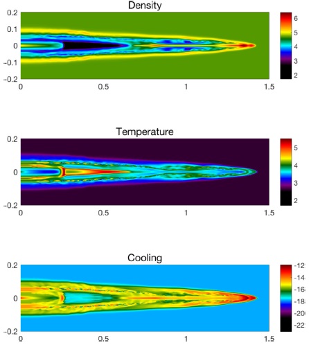
Fig. 2 Log10(n) of density with n in H atoms/cm3 (top panel), log10(T) of temperature with T in K (middle panel), and log10(C) of total radiative cooling with C in erg cm−3 s−1 (bottom panel) at t = 35 yr. Lengths along the boundaries are in units of 1011 km. The HST observations extend out to 0.94 × 10¹¹ km = 4.5 arcsec. The color figure can be viewed online.
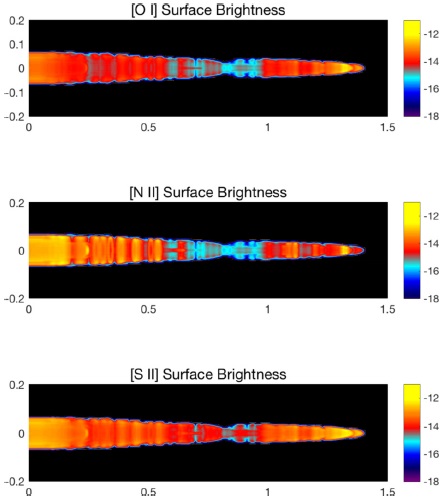
Fig. 3 Simulated surface brightness S in the [O I] (6300 + 6363 ̊A) doublet (top panel), [N II] (6584 + 6548 Å) doublet (top panel), [N II] (6584 + 6548 Å) doublet (middle panel), and [S II] (6716 + 6731 Å) doublet (bottom panel) at 35 yr, projected 80◦ with respect to the line of sight: log10(S) with S in erg cm-2 arcsec-2 s-1. Lengths along the boundaries are in 1011 km. The HST observations extend out to 0.94 × 10¹¹ km = 4.5 arcsec. The color figure can be viewed online.
The HH 30 jet is one of the densest jets observed (Bacciotti et al. 1999). Observationally the jet density starts at 105 H/cm3, decreases to 5 × 10⁴ H/cm3 within the first arcsec (= 2.1 × 10¹⁰ km), and then gradually falls to 104 H/cm3 at a few arcsec; the jet temperature starts at 2 × 10⁴ K, decreases to 104 K within the first arcsec, and then gradually decays to 6000-7000 K at a few arcsec. These data are well matched by our simulated densities and temperatures in Figure 2 out to the limit of the HST observations at 0.94 × 10¹¹ km = 4.5 arcsec.
Figure 3 presents our simulated surface brightness of the jet in the three forbidden doublets, projected onto the plane of the sky. The surface brightness has been smoothed with a Gaussian pointspread function with a width of 0.1 arcsec. Qualitatively the simulations are similar to the observations of Hartigan and Morse (2007), but the real test is to compare surface brightness in each doublet along the center of the jet.
4. DISCUSSION
As is evident in Figures 2 and 3, the jet pulses create a series of shocked knots followed by rarefactions within the jet. In Figure 2, the panels indicate shocked knots at z ≈ 0.25, 0.8, 1.0, and 1.4 × 10¹¹ km, with an incipient knot beginning at z = 0. The incipient knot plus the next three knots correspond to the N, A, B, C knots illustrated in Hartigan and Morse (2007), while the final knot is outside the spatial range of their observations. In our simulations, the jet creates a terminal Mach disk near the jet tip, which reduces the velocity of the jet flow to the flow velocity of the contact discontinuity at the leading edge of the jet. With radiative cooling, the jet exhibits a higher density contrast near its tip (when the shocked, heated gas cools radiatively, it compresses), a narrower bow shock, and lower overall temperatures. There is a strong rarefaction for z ≈ 0.25 − 0.7 × 10¹¹ km between knots A and B. The knots at z ≈ 0.25, 0.8, and 1.1 × 10¹¹ km are undergoing especially strong radiative cooling. The temperature is highest around the knot at z ≈ 0.25 and for the strong rarefaction between z ≈ 0.25 − 0.7 × 10¹¹ km. In Figure 3, there is strong cooling in all three doublets for 0 ≤ z ≤ 0.7×10¹¹ km and for 1.0 × 10¹¹ ≤ z ≤ 1.4 × 10¹¹ km. The [O I] doublet emission is low for 0.8×10¹¹ ≤ z ≤ 1.0×10¹¹ km, while the [N II] doublet emission is low for 0.7×10¹¹ ≤ z ≤ 1.0 × 10¹¹ km.
In computing the emission lines, the density of each ionic species is calculated by Cloudy assuming local ionization/recombination equilibrium in each grid cell. The approach to equilibrium of an ionized gas is characterized by various timescales-see Spitzer (1962) and the documentation for Cloudy (Ferland et al. 2013). For near nebular conditions (T ≈ 104 K and n ≈ 104 H/cm3), the longest is the H+ recombination time, which in this regime is
where ne is the electron density. To be near ionization/recombination equilibrium, the equilibrium time tequil ≈ trec should be short compared to the cooling time tcool = E/|dE/dt| = E/C. Figure 7 plots the ratio of the recombination time to the cooling time at t = 35 yr. In most of the jet, trec /tcool ≤ 10−1. The bow shocks from the various pulses are visible as thin red/orange ⊃-shaped shells. Except for the innermost first shell for 0 ≤ z ≤ 0.25 from the last full knot, the shells are so thin they do not significantly affect the emission line calculations. There are two regions of concern: First, in the strong, triangular-shaped rarefaction for z ≈ 0.25−0.7×10¹¹ km between knots A and B, trec /tcool ≈ 10. However, because this region is a rarefaction, n and n e are low, and radiative cooling (see the bottom panel of Figure 2) is suppressed by more than a factor of 100 with respect to the immediately surrounding regions. Second, in the ⊃-shaped bow shock for 0 ≤ z ≤ 0.25 from the last full knot, there is significant far-from-equilibrium (trec /tcool ≈ 1) radiative cooling, which may distort the surface brightness results for that region. There are some discrepancies in the simulated surface brightness along the center of the projected jet for each doublet out to 1.2 arcsec, but no worse than in other regions. We believe this validates the gas dynamical/Cloudy methodology for the HH 30 jet.
The multiple-ion MHD simulations of Tesileanu et al. (2014) yield good qualitative agreement with the A, B, C knot structure of the HH 30 jet over the first 0.003 pc. Figures 4-6 present the comparisons of surface brightness in each of the three doublets along the center of the projected jet for observational data (labeled “obs”, from the data of Hartigan and Morse 2007), MHD multiple-ion simulations (labeled “T sim”, Tesileanu et al. 2014), and our gas dynamical/Cloudy simulations smoothed over 0.2 arcsec (labeled “our sim”). Our simulated surface brightness is always within ±7.5% on the logarithmic scale of the observational data for the [O I], [S II], and [N II] forbidden doublets; in addition, the general trend of our simulated surface brightness maps closely follows the observational patterns from the limit of the HST data at 4.5 arcsec all the way up to the circumstellar disk.
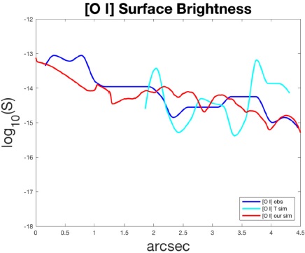
Fig. 4 Log10(S) of surface brightness in the [O I] (6300 + 6363 Å) doublet along the center of the projected jet, with S in erg cm−2 arcsec−2 s−1. Length scale is in arcsec from the source, with 1 arcsec = 2.1 × 10¹⁰ km. The color figure can be viewed online.
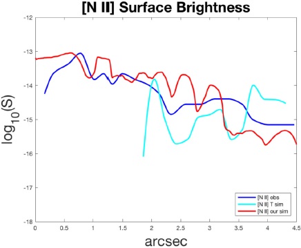
Fig. 5 Log10(S) of surface brightness in the [N II] (6584 + 6548 Å) doublet along the center of the projected jet, with S in erg cm−2 arcsec−2 s−1. Length scale is in arcsec from the source, with 1 arcsec = 2.1 ×10¹⁰ km. The color figure can be viewed online.
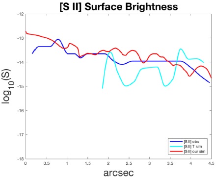
Fig. 6 Log10(S) of surface brightness in the [S II] (6716 + 6731 Å) doublet along the center of the projected jet, with S in erg cm−2 arcsec−2 s−1. Length scale is in arcsec from the source, with 1 arcsec = 2.1 × 10¹⁰ km. The color figure can be viewed online.
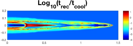
Fig. 7 Log10 (trec /tcool) of the ratio of the H+ recombination time to the cooling time at t = 35 yr. Lengths along the boundaries are in units of 1011 km. The HST observations extend out to 0.94 × 10¹¹ km = 4.5 arcsec. The color figure can be viewed online.
Photoionization does not appear to be important close to the circumstellar disk: according to Hartigan & Morse (2007), heating of the jet is not caused by photoionization from the stellar source/disk, because the ionization fraction is initially low near the source (≤ 10% within 20 AU of the star) and increases further outward along the jet (30%-40% at 100 AU from the star).
Earlier gas dynamical simulations including radiative cooling of the HH 30 jet are presented in Esquivel et al. (2007) and de Colle (2011). While the simulations of Esquivel et al. (2007) model the largescale structure of the jet and the chain of emission knots out to 0.22 pc, the simulations do not have enough resolution to model the detailed knot structure of the jet near its launch site (≤ 0.003 pc). The simulations of de Colle (2011) do produce good qualitative agreement with the A, B, C knot structure of the jet over the first 0.003 pc, but quantitatively the jet densities are too large by a factor of 5 near 0.003 pc.
Tesileanu et al. (2014), Esquivel et al. (2007), and de Colle (2011) all sinusoidally modulate the inflow jet velocity, with periods of 3.7, 2.5, and 3 yr, respectively, while our simulations employ a period of 8yr,with the jet on for 6.5yr and off for 1.5 yr periodically. Our sequencing of the jet pulses produces a better fit with the HST observations. Furthermore, pulsing the jet with a simple periodic on/off injection better matches the observed behavior of pulses from many HH jets over long epochs, most dramatically perhaps from HH 24 and HH 34, and seems to be a simpler and more physical modeling of infall of disk matter into the jet source.
5. CONCLUSION
Simulating the HH 30 astrophysical jet with a gas dynamical solver with radiative cooling and then post-processing the simulated densities and temperatures with Cloudy produces simulated surface brightness maps that are in excellent agreement with the HST observations of Hartigan and Morse (2007). On a logarithmic scale, our surface brightness simulations along the center of the jet are always within ±7.5% of the observational data for all three doublets, and fit the observational data more tightly than the simulations of Tesileanu et al. (2014). In addition, the general trend of our simulated surface brightness in each doublet closely follows the observational data, confirming our choices of initial jet and ambient densities and jet temperature and the number of and sequencing of the jet pulses during the 35 year evolution of the jet within the first 0.003 pc of its launch site.

