1. INTRODUCTION

Gamma ray bursts are related to extremely energetic explosions in far away galaxies (for reviews, see ^{Wang et al. 2015}; ^{Wei & Wu 2017}; ^{Petitjean et al. 2016}). Based on the collapse model which proposes the formation of long-GRBs by the collapse of a rapidly rotating super massive star (e.g. Wolf-Rayet star M > 20M_⊙, for cosmological implications of GRBs see ^{Wei & Wu 2017} and ^{Wei et al. 2016}) we can trace and test the SFR (^{Yüksel et al. 2008}) (^{Kistler et al. 2008}) (^{Wang 2013}) related with this events. The study of SFR through traditional tracers, such as continuous UV (^{Cucciati et al. 2012}), (^{Schenker et al. 2013}), (^{Bouwens et al. 2014}), recombinacion lines of: Hα, far infrared (^{Magnelli et al. 2013}), (^{Gruppioni et al. 2013}), radio and Xray emission, are inefficient at high redshift (z > 4) (^{Schneider 2015}) due to their sensitivity to extinction for gas and dust and the expansion of the universe.

The stellar formation activity in the universe was very intense in the past, higher than now; at z ∼ 2.5 about 10% of all stars were formed and about 50% of the local universe star formation took place at z ∼ 1, (^{Schneider 2015}). The star formation rate density is a function which evolves with time. It has shown an increase of a factor 10 between now and z ∼ 1 holding until z ∼ 3−4 and finally a decrease at z > 4 (^{Hopkins & Beacom 2006}; ^{Carroll & Ostlie 2006}; ^{Schneider 2015}). Figure 1 shows the distribution of our sample with redshift. The data presenta mode at z ≈ 1.17 and a mean at z ≈2.06. These results match the observational data.

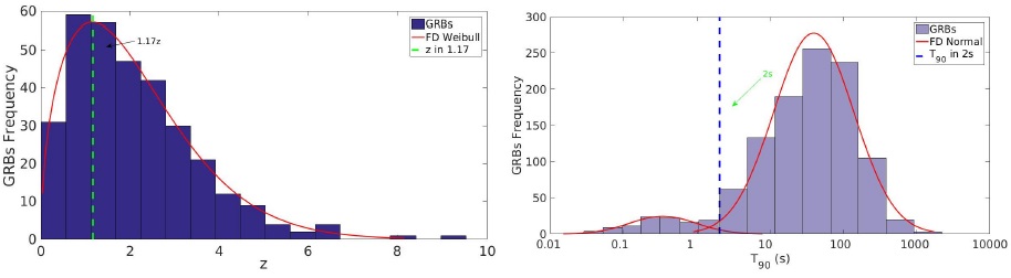
Fig. 1 Left Frequency histogram of 333 long-GRBs over z. The data show a mode at 1.17z and a mean at z = 2.06. These results match the observational data. Right Bimodal distribution of our sample made up by 994 long-GRBs; we can see both types of GRBs (long T₉₀ > 2s and short T₉₀ < 2s). The color figure can be viewed online. 

The paper is organized as follows. In § 2 we present the main properties of our long-GRBs sample. In § 3 we develop the mathematical model to calculate the SFR using long-GRBs as a tracers. In § 4 we present the results based on the computation of δ obtained by a linear regression analysis over the long-GRB sample. Our conclusions are in § 5.

2. DESCRIPTION OF THE SAMPLE

The data sample used includes 959 GRBs observed by Swift supplied by ^{Butler et al. (2017)} and 35 bursts detected by FERMI from ^{Narayama Bhat et al. (2016)} and ^{Singer et al. (2015)}, BeppoSAX from ^{Frontera et al. (2009)} and ROTSE from ^{Rykoff et al. (2009)} giving a total of 994 GRBs; 333 are long-GRBs with T₉₀ and z established; from these only 263 present an isotropical energy E_iso already defined. We consider bursts up to 2017 June 4. Figure 1 shows the data considered, as observed by BATSE. The bimodal distribution allows to define the short and long-GRBs.

3. DERIVATION OF THE SFR USING GRBS

The conversion factor between the GRBs rate and the SFR is hard to identify, but it is supported by an increasing amount of data of the cosmic star formation rate at low redshift z < 4 (^{Cucciati et al. 2012}; ^{Dahlen et al. 2007}; ^{Magnelli et al. 2013}) and the relationship between long-GRB and star formation. Based on the hypernova model we can relate the observed GRBs at low redshift with the SFR measurements considering an additional evolution of the GRBs rate with the SFR (^{Kistler et al. 2008}; ^{Yüksel et al. 2008}).

The GRBs distribution per unit redshift over all sky is given by:

where 0 < F(z) < 1 is the probability to obtain the redshift related to an afterglow from their host galaxy. ε(z) is the long-GRBs rate production with additional evolution effects, fbeam is the number of GRBs that are observed due to their beaming, ρ˙*(z) is the SFR density, where the dot represents comoving coordinates, 1/(1+z) is a factor related to cosmological time dilation, dV_com /dz¹ is the differential volume in comoving coordinates per redshift unit. ε(z) is parameterized as ε(z) = ε₀(1 + z)^δ, where ε₀ is a constant which includes the absolute conversion from SFR to GRB in a GRB luminosity range, and δ is the slope left by the trace of the SFR in a redshift range.

Table 1 presents 10 elements of the sample, listing some spectral properties such as Energy Fluence², Peak Energy Flux³, Peak Energy Flux⁴E_iso, Ep and T ₉₀. Using E_iso we can obtain the isotropical luminosity L_iso by equation 2

In Figure 2 we present the luminosity distribution of our sample made up by 263 long-GRBs. Here we observed the relation between (L_iso) with redshift considering that only highly luminous GRBs can be seen at high z, using a luminosity boundary of L_iso > 10⁵¹ergs⁻¹ established by ^{Kistler et al. (2008)}. The spatial distribution of the events is shown in 5 redshift bins 1−4,4−5,5−6,6−8 and 8 − 10, where we will calculate the SFR.

Fig. 2 Distribution of 263 long-GRBs detected by Swift from Butler et al. (2007). We highlight 5 areas used to estimate the SFR density at different redshift bins (1 − 4,4 − 5,5 − 6,6 − 8,8 − 10) as discussed in the text, with (173,15,4,2) bursts, respectively. The color figure can be viewed online. 

The theoretical accounts of GRBs in the range of redshift from 1 to 4 are expressed by equation 3⁵

where

A depends on the total observed time by Swift ∆t and on the angular sky coverage ∆Ω. Utilizing the SFR overage density ρ˙*z1-z2 we compute the theoretical numbers of GRB in a range of redshift from z₁ to z₂, which is given by

Taking the calculation of GRBs observed Nz1-z2obs we obtain the SFR in a specific range of z, z₁− z₂, and using the bin 1−4 we determine the SFR overage density with equation 5

4. DESCRIPTION OF THE SFR MODEL BY LONG-GRBS

Considering the results obtained by ^{Hopkins & Beacom (2006)} and studies made by ^{Yu et al. (2015)} about the GRBs rate compared with SFR we defined the best fit to δ in different ranges of z, where the best fit to ρ˙* is given in Table 2.

We calculate ρ˙*z parameterized as a function of redshift and δ using a power law, considering that we are including a larger range of redshift and also a larger number of long-GRBs than ^{Yüksel et al. (2008)}. We extend their model with equation 6 adding the term η representing the overage account of long-GRBs observed in the bin of z (z₁, z₂) normalized by the number of long-GRBs in the bin (1,4)

where ρ˙+ ( is given by equation 7 proposed by ^{Yüksel et al. (2008)}; in order not to lose consistency we use ρ˙+ as ρ˙*:

Here, the constants a,b and c include the logarithmic slope δ of the track left by ρ˙*z (see Table 2); the normalization is ρ˙0=0.02M⊙ yr^-1 Mpc^-3 and τ ≈ −10. (see ^{Yüksel et al. 2008} for more details). We define B and C with the next expressions:

Our first approximation of the density ρ˙*(z), using the best fit of δ from the literature (see Table 2) is

In Figure 3 is shown the σ confidence interval. The update to the SFR in a specific range of z of ^{Yüksel et al. (2008)} used in this work is described by the next equation:

Fig. 3 Top: logarithmic distribution of ρ˙*(z) vs. redshift. We present the results and a comparison between different tracers. Results are plotted as red solid diamonds, and those obtained in the UV and FIR are also plotted. The purple region represents the confidence interval with 1σ of significance and the black line represents the total SFR density fit with the equation log₁₀ρ˙* = -0.002z⁴ + 0.053z³ - 0.414z² + 1.101z - 1.764 Bottom: Residual plot of log⁡ρ˙*(z) we note a significant high dispersion at high redshift (z > 5). The symmetrical distribution shows a good fit to the data. The color figure can be viewed online. 

4.1. Statistical Analysis of the Model

Considering that δ, which is the slope left by the trace of the SFR function in a redshift range, is not constant, and taking account the relation between a GRB of stellar origin by the hypernova model (^{Schneider 2015}; ^{Carroll & Ostlie 2006}) we calculate these δs directly from the sample through a linear regression over the z bins 0−1,1−4 and 4−10, where the regions have 89,214, and 30 events, respectively, and since z has 3 significant digits, we did the analysis using grouped data.

We calculated the frequency table of each bin and their respective histogram, which lets us obtain the linear regression over the data, and their respective slope. In the bin 0 − 1 with 89 burst we obtain the linear equation y = 2.32x + 3.4286; in the bin 1 − 4, with 214 burst we obtain the linear equation y = −1.0643x + 22.781; and in the bin 4 − 10, with 30 burst we obtain the linear equation y = −4x+18. Proceeding with the analysis we calculated the confidence interval over one σ of significance, obtaining the best fit to the model at different ranges of z. This is shown in Table 2.

Based on the results of the statistical analysis we calculated the density ρ˙*z and the average density ρ˙*z1-z2. In Figure 3 and 4 we compare the results with the ones obtained by traditional tracers summarized by ^{Madau & Dickinson (2014)}.

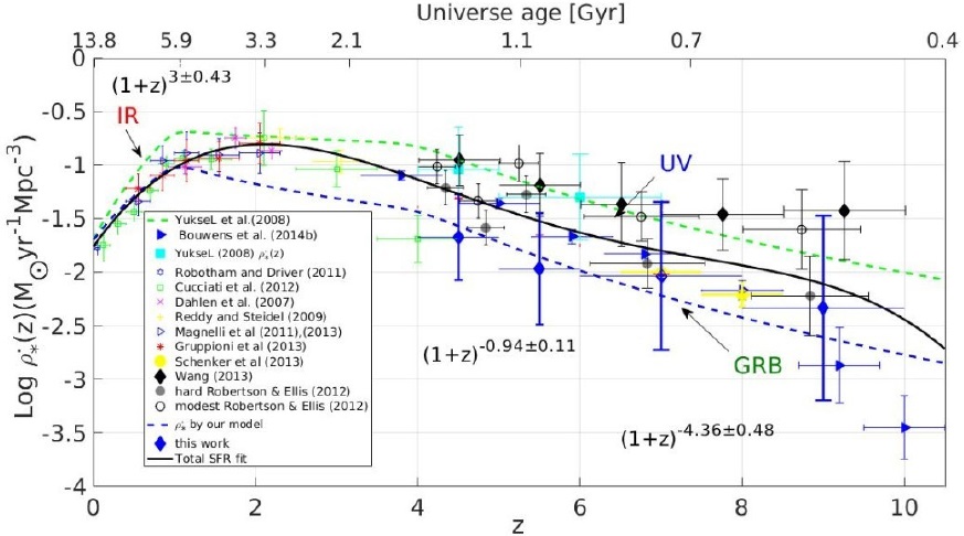
Fig. 4 Logarithmic distribution of the SFR log⁡ρ˙*(z) vs. redshift analogous to Figure 3. We present the results and a comparison between different tracers. Our results are plotted as blue solid diamonds using δ indexes from our statistical analysis; the black line represents the total SFR density fit. The color figure can be viewed online. 

5. DISCUSSION AND CONCLUSION

In this paper we presented the results of our work based on the estimation of the SFR through a mathematical model which relates a GRB directly with a stellar origin. We used the latest Swift catalog supplied by ^{Butler et al. (2017)}. Based in the distribution of L_iso (see Figure 2) we computed the SFR using first the values of δ from the literature (see Figure 3). We made a linear regression analysis with our long-GRB sample reproducing the reported δ indexes (see Table 2). Using these results we computed new values for the SFR average density ρ˙*z1-z2. We are including a bigger range of redshift than ^{Yüksel et al. (2008)} and a larger number of long-GRBs than ^{Wang (2013)}. We extended the model adding a new term η (see equation 9). Our results were compared with the results from traditional tracers, such as UV and FIR (see Figure 4). Some other results, such as ^{Robertson & Ellis (2012)} found higher and similar values of ρ˙* at z > 4 than ours based on a modest and hard evolution of the SFR with δ = 0.5 and δ = 1.5 respectively, and considering GRBs from low metalicity host galaxies with 12 + log[O/H] ≈ 8.7 (^{Savaglio et al. 2005}). Their results with δ = 0.5 and δ = 1.5 are shown as open black circles and solid gray circles in Figures 3 and 4. Our results can be marginally consistent with the gray circles. Wang (2013) used a sample of 110 luminous Swift GRBs to find an index value of δ ≈ 0.5 based on GRBs produced by rapidly rotating metal-poor stars with low mass; their SFR is higher than our results. This may be a consequence of the update used for the Swift GRB sample in our work and of the type of model proposed for the estimation of SFR, considering that our model is highly dependent on the selected index value δ at different redshift bins. With regard to the physical implication and the results obtained along this work we conclude the next points.