nueva página del texto (beta)
 Inglés (pdf)
 Artículo en XML
 Referencias del artículo
 Enviar artículo por email
 Citado por SciELO
  Similares en
SciELO
Similares en
SciELO 
 Permalink
1. Introduction
Active galactic nuclei (AGNs) are among the most energetic processes in the Universe. Being powered by the accretion of matter into a super-massive black hole (SMBH; M > 106 M⊙ ) that resides in the center of most galaxies, they can be as luminous as their host galaxies, or even more, outshining the light of all the stars together (e.g Jahnke et al. 2004a). In essence, they are characterized by a luminous pointlike source residing in the center of the host galaxy.
In the optical range, the AGN spectra may exhibit a characteristic power-law continuum together with a set of strong nuclear emission lines, signatures of high ionization. The characteristics of the emission lines depend on the kind of AGN and allow their classification as follows: (i) Type-I AGNs: the permitted lines can present broad components with a width of several thousands of km/s (≈ 1000 − 10000 km/s), usually with a narrow component superposed to the broad one. (ii) Type-II AGNs: only narrow components with a width that does not exceed 1200 km/s. (iii) Blazars: no lines except when a highly variable continuum is in a low phase (BL LAC objects and optically violently variable QSOs, OVVs).
In addition, many radio-loud AGNs do not present any evidence for the presence of the central source in the optical range, exhibiting a perfectly normal stellar-dominated spectrum. The undoubted signature of the presence of an AGN is the hard Xray radiation, which is a signature of thermal, synchrotron, and high energetic radiation processes that happen in the accretion disk surrounding the black hole. However, the shallow detection limit of many X-ray observations affects the detectability of that feature.
The exotic emission shown by AGNs and the relatively small fraction of AGNs in the Local Universe (≈1-3% for type-I AGNs and ≈20% for type-II ones, if we include LINERs) has constrained the scope of their study to the characterization of peculiar nonthermal sources in a limited number of objects. In other words, AGNs did not seem to play any significant role in the overall evolution of galaxies. However, three observational results have changed that view in the last decades: (i) the presence of strong correlations between the mass of the central black hole and the properties of the host galaxy, such as bulge luminosity, mass and velocity dispersion (see for recent reviews Kormendy & Ho 2013; Graham 2016); (ii) the need of an energetic process able to remove or heat gas in massive galaxies in order to halt their growth by star formation (SF) and reconcile in this way the high-mass end of the observed galaxy mass (luminosity) functions with those derived by means of semi-analytic models of galaxy evolution (e.g., Kauffmann & Haehnelt 2000; Bower et al. 2006; Croton et al. 2006; De Lucia & Blaizot 2007; Somerville et al. 2008) and cosmological simulations (e.g., Sijacki et al. 2015; Rosas-Guevara et al. 2016; Dubois et al. 2016); and (iii) the need for a fast (≤1 Gyr) morphological transformation between spiral-like star-forming galaxies and dead ellipticals in the last 8 Gyrs based on the number counting and luminosity distributions of both families of galaxies in different surveys (e.g., Bell et al. 2004; Faber et al. 2007; Schiminovich et al. 2007). All together, these results strongly suggest that SMBHs co-evolve with galaxies or, at least, with their spheroidal components (see e.g. Kormendy & Ho 2013), and therefore AGN feedback seems to be an important phase in galaxy evolution. Indeed, AGN negative feedback has been proposed as a key process to heat/eject gas, halt SF, and transform galaxies between different families (Silk & Rees 1998; Silk 2005; Hopkins et al. 2010). Actually, it may explain the evolutionary sequence between central low-ionization emission-line regions (LIERs) and extended LIERs proposed by Belfiore et al. (2017).
Different observational results seem to support the scenario mentioned above. Kauffmann et al. (2003a) showed that type-II AGNs selected from the SDSS sample were located in the so-called “green valley” (GV) of the color-magnitude diagram (CMD), that is, in the expected location for transitory objects between the blue cloud of starforming galaxies (SFGs) and the red sequence of retired/passive ones (RGs). These results were confirmed with a more detailed analysis of the host galaxies at intermediate redshift by Sánchez et al. (e.g., 2004b), showing that type-I AGNs seem to be at the same location too. These results have been updated by more recent studies (e.g. Schawinski et al. 2010; Torres-Papaqui et al. 2012, 2013; Ortega-Minakata 2015). Indeed, such results indicate that AGN hosts are located in the intermediate/transitory regions in other diagrams, like the SF vs. stellar mass (for a recent study see e.g., CanoDíaz et al. 2016). However, the possibility that these galaxies are found in the reported location due to a contamination by the AGN itself cannot be ruled out, as this effect has not been studied in detail. Another caveat is that, in general, the simplistic picture that all AGN hosts present evidence of recent interactions is known not to be true for most Seyfert galaxies (e.g. Hunt & Malkan 1999), not even for the stronger type-I QSOs (e.g. Sánchez et al. 2004b; Böhmetal.2013). Finally,afundamentalproblem arises when comparing the properties of active and non-active galaxies. If the AGN activity is a short-lived recurrent process in galaxies - compared with Hubble time - as it is assumed today, then any galaxy without an AGN could have had one in the past. Thus, any comparison between both families is only restricted to the current effects of the AGN activity on the overall evolution, and it is not possible to determine which effect may have occurred in the past. Therefore, the fact that AGN hosts are located in particular regimes of galaxy properties is even more puzzling considering its recurrent and transitory nature.
In order to address these questions, we present here a study of the main properties of the galaxies with AGN detected in the MaNGA/SDSS-IV survey (Mapping Nearby Galaxies at the Apache Point Observatory, Bundy et al. 2015). We study in detail their global and radial properties compared with those of the full sample of galaxies observed by this survey; we focus on the comparison of their structural (e.g., morphology, concentration) and dynamical properties (rotational vs. pressure support), and in particular their state in terms of current and recent SF activity, and its relation with the molecular gas content in these galaxies.
Recently, Rembold et al. (in prep.) studied the AGNs on the MaNGA sample using a different approach. They selected a control sample of two galaxies for each active one. They matched the properties of the host galaxies, such as mass, distance, morphology and inclination, in order to investigate if there are any stellar population properties related to the AGN alone regardless of the galaxy type. They found a correlation of the galaxy stellar population properties - such as the contribution from different age bins as well as the mean age - with the luminosity of the AGN. This work can be considered complementary to ours, as in our paper we aim to compare the host properties, including the stellar population, to those of all non-active galaxies of the MaNGA sample.
This paper also aims to present a Value Added Catalog (VAC) that is part of the 14th Data Release of SDSS (Abolfathi et al. 2017) for the MaNGA galaxies. The dataproducts presented in the VAC were produced by the Pipe3D pipeline (Sánchez et al. 2016a).
This article is structured in the following way: In § 2 we describe the sample and the currently used dataset; § 3 summarizes the main steps of the performed analysis. In § 3.5 we describe the AGN hosts selection and the different groups in which we have classified the sample of comparison galaxies. § 4 shows the main results, presented in the following subsections: (i) § 4.1 shows which kind of galaxies host AGNs; (ii) § 4.2 demonstrates that they are located in the GV; (iii) § 4.4 shows the deficit of molecular gas in these galaxies; (iv) § 4.5 and 4.6 show the radial distribution of the SF rate (SFR) and molecular gas content, demonstrating that the quenching of SF happens from inside-out, and finally (v) § 4.7 compares the AGN hosts with the non-active galaxies in the GV. The results are discussed in § 5, and the main conclusions are presented in § 6. The contents of the distributed dataproducts included in the SDSS-DR14 VAC are described in Appendix A, and the catalog of AGN candidates is included in Appendix A.2.
Along this article we assume the standard Λ Cold Dark Matter cosmology with the parameters: H0=71km/s/Mpc,ΩM=0.27,ΩΛ=0.73. Finally, Table 1 lists all the acronyms used in this paper, including the ones of the surveys/catalogs mentioned here.
Table 1 List of acronyms used in this paper
| AGN | Active Galactic Nuclei |
| BLR | Broad Line Region |
| BPT | Baldwin, Phillips & Terlevich diagram |
| CMD | Color-Magnitude Diagram |
| EW | Equivalent Width |
| FoV | Field of View |
| FWHM | Full Width at Half Maximum |
| GV | Green Valley |
| IFS | Integral Field Spectroscopy |
| IFU | Integral Field Unit |
| ISM | Interstellar Medium |
| LINERs | Low-Ionization Nuclear Emission-line Regions |
| IMF | Initial Mass Function |
| MZR | Mass-Metallicity Relation |
| NLR | Narrow Line Region |
| PSF | Point Spread Function |
| RG | Retired Galaxy |
| S/N | Signal-to-noise ratio |
| SFE | Star Formation Efficiency |
| SFG | Star-Forming Galaxy |
| SFMS | Star-forming Main Sequence |
| SFR | Star Formation Rate |
| sSFR | Specific Star Formation Rate |
| SMBH | Super-Massive Black Hole |
| SSP | Single Stellar Population |
| DR | Data Release |
| CALIFA | Calar Alto Legacy Integral Field spectroscopy Area survey |
| MaNGA | Mapping Nearby Galaxies at APO |
| NSA | NASA-Sloan Atlas |
| SDSS | Sloan Digital Sky Survey |
| VAC | Value Added Catalog |
2. Sample and data
We use the sample observed by the MaNGA (Bundy et al. 2015) survey until June 2016 (so called MPL-5 sample). MaNGA is part of the 4th version of the Sloan Digital Sky Survey (SDSS-IV Blanton et al. 2017). The goal of the ongoing MaNGA survey is to observe approximately 10,000 galaxies; a detailed description of the selection parameters can be found in Bundy et al. (2015), including the main properties of the sample, while a general description of the Survey Design is found in Yan et al. (2016a). The sample was extracted from the NASA-Sloan atlas (NSA, Blanton M. http://www.nsatlas.org).
Therefore, all the parameters derived for those galaxies are available (effective radius, Sersic indices, multi-band photometry, etc.). The MaNGA survey is under way at the 2.5 meter Apache Point Observatory (Gunn et al. 2006). Observations are carried out using a set of 17 different fiber-bundles science integral-field units (IFU; Drory et al. 2015). These IFUs feed two dual channel spectrographs (Smee et al. 2013). Details of the survey spectrophotometric calibrations can be found in Yan et al. (2016b). Observations were performed following the strategy described in Law et al. (2015), and reduced by a dedicated pipeline described in Law et al. (2016). These reduced datacubes are internally provided to the collaboration trough the data release MPL-5. This sample includes more than 2700 galaxies at redshift 0.03< z <0.17, covering a wide range of galaxy parameters (e.g, stellar mass, SFR and morphology), and provides a panoramic view of the properties of the population in the Local Universe. For details on the distribution of galaxies in terms of their redshifts, colors, absolute magnitude and scale-lengths, and a comparison with other on-going or recent IFU surveys, see Sánchez et al. (2017).
3. Analysis
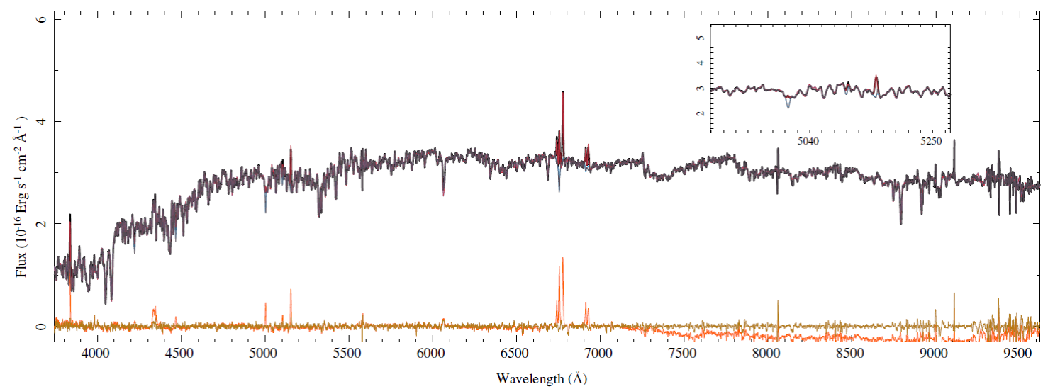
We analyze the datacubes using the Pipe3D pipeline (Sánchez et al. 2016a), which is designed to fit the continuum with stellar population models and to measure the nebular emission lines of IFS data. This pipeline is based on the FIT3D fitting package (Sánchez et al. 2016b). The current implementation of Pipe3D adopts the GSD156 library of simple stellar populations (SSPs Cid Fernandes et al. 2013), that comprises 156 templates covering 39 stellar ages (from 1Myr to 14.1Gyr), and 4 metallicities (Z/Z⊙=0.2, 0.4, 1, and 1.5). These templates have been extensively used by the CALIFA collaboration (e.g. Pérez et al. 2013; González Delgado et al. 2014b), and by other surveys. Details of the fitting procedure, dust attenuation curve, and uncertainties on the processing of the stellar populations are given in Sánchez et al. (2016b,a).
In summary, a spatial binning is first performed in order to reach a S/N of 50 across the entire field of view (FoV) for each datacube. A stellar population fit of the co-added spectra within each spatial bin is then computed. The fitting procedure involves two steps: first, the stellar velocity and velocity dispersion are derived, together with the average dust attenuation affecting the stellar populations (AV,ssp). Second, a multi-SSP linear fitting is performed, using the library described before and adopting the kinematics and dust attenuation derived in the first step. This second step is repeated including perturbations of the original spectrum within its errors; this Monte-Carlo procedure provides the best coefficients for the linear fitting and their errors, which are propagated for any further parameter derived for the stellar populations.
We estimate the stellar population model for each spaxel by re-scaling the best fitted model within each spatial bin to the continuum flux intensity in the corresponding spaxel, following Cid Fernandes et al. (2013) and Sánchez et al. (2016b). This model is used to derive the average stellar properties at each position, including the actual stellar mass density, lightand mass-weighted average stellar age and metallicity, and the average dust attenuation. In addition, the same parameters are derived accross the look-back time, which comprises in essence the SF and chemical enrichment histories of the galaxy at different locations. In this analysis we followed Sánchez et al. (2016a), but also Cid Fernandes et al. (2013), González Delgado et al. (2016), González Delgado et al. (2017) and García-Benito et al. (2017). In a way similar to Cano-Díaz et al. (2016) it is possible to co-add, average, or azimuthally average those parameters to estimate their actual (and/or time evolving) integrated characteristics or radial distributions.
The stellar-population model spectra are then subtracted from the original cube to create a gaspure cube comprising only the ionised gas emission lines (and the noise). Individual emission line fluxes are then measured spaxel by spaxel using both a single Gaussian fitting for each emission line and spectrum, and a weighted momentum analysis, as described in Sánchez et al. (2016a). For this particular dataset, we extract the flux intensity and equivalent widths of the following emission lines: Hα, Hβ, [O ii] λ3727, [O iii] λ4959, [O iii] λ5007, [O i] λ6301, [N ii] λ6548, [N ii] λ6583, [S ii]λ6717 and [S ii]λ6731 (although a total of 52 emission lines are analyzed Sánchez et al. 2016a). All those intensities are corrected for dust attenuation. To do that, the spaxelto-spaxel Hα/Hβ ratio is used. Then, a canonical value of 2.86 for this ratio (Osterbrock 1989), is assumed and adopting a Cardelli et al. (1989) extinction law and a RV=3.1 (i.e., a Milky-Way-like extinction law), the spatial dust attenuation in the V-band (AV,gas) is derived. Finally, using the same extinction law and derived attenuation, the correction for each emission line at each location within the FoV is applied.
All the parameters derived by Pipe3D for the ≈2700 galaxies/cubes studied here, including the average, integrated and characteristic values and their spatial distributions, are publicly accessible through the SDSS-IV Value Added Catalog (VAC) web-site as described in Appendix A. In addition to the parameters described before we have derived the following properties, also included in the distributed VAC.
3.1. Star Formation Rate
The SFR and SFR surface densities, ΣSFR, are derived using the Hα intensities for all the spaxels with detected ionized gas. The intensities are transformed to luminosities (using the adopted cosmology) and corrected by dust attenuation as indicated below. Finally we apply the Kennicutt (1998) calibration to obtain the spatially-resolved distribution of the SFR surface density. We use all the spaxels irrespectively of the origin of the ionization. By doing so, we take into account the PSF wings in the starforming regions, that may present equivalent widths below the cut applied in Sánchez et al. (2017) and Cano-Díaz et al. (2016) (as we will explain the following sections). On the other hand, we are including in our SF measurement regions that are clearly not ionized by young stars. For SFGs that contribution is rather low, due to the strong difference in equivalent widths, as already noticed by CatalánTorrecilla et al. (2015), and therefore the SFR is only marginally affected. However, for the RGs, the ionization comes from other sources, including AGN ionization, post-AGB stars, or rejuvenation in the outer regions (e.g Sarzi et al. 2010; Papaderos et al. 2013; Singh et al. 2013; Gomes et al. 2016a,b; Belfiore et al. 2017). Therefore, the Hα-based SFR for RGs should be considered as an upper limit. However, for the main goals of this study (comparing the properties of the AGN hosts to thoe of the overall population) that value is good enough. In general, the reported SFRs (and densities) should be considered as just a linear transformation of the Hα luminosity (or surface density luminosity).
3.2. Oxygen Abundances
The spatially-resolved oxygen abundances are derived only in those spaxels whose ionization is compatible with being produced by star-forming areas, following Sánchez et al. (2013). For this, we select those spaxels located below the Kewley et al. (2001) demarcation curve in the classical BPT diagnostic diagram ([O iii]/Hβ vs [N ii]/Hα diagram, Baldwin et al. 1981), and with a EW(Hα) larger than 6ºA. These criteria ensure that the ionization is compatiblewiththatduetoyoungstars(Sánchezetal. 2014). Then, we use different line ratios to derive the oxygen abundance using the so-called t2 calibration following Sánchez et al. (2017). In essence, this calibrator averages the oxygen abundances derived with the R23 line ratio, O3N2 and N2 calibrators (Marino et al. 2013), and the ONS one (Pilyugin et al. 2010), and corrects them using a rough estimation of the effect of the temperature inhomogeneities in the ionized nebulae following Peimbert & Peimbert (2006). In addition, we derive the oxygen abundance using a total of 7 calibrators, described in Sánchez et al. (2017), for comparison purposes. However, along this article we will describe only the results based on the t2 calibrator. For the remaining ones, the results were quantitatively different but qualitatively similar.
3.3. Molecular Gas Estimation
The cold molecular gas is a very important parameter to understand the SF processes since it is the basic ingredient from which stars are formed (see e.g., Kennicutt & Evans 2012; Krumholz et al. 2012). Indeed, the well known Schmidt-Kennicutt law that shows the correlation of the integrated gas mass (molecular+atomic) with the integrated starformation rate (e.g. Kennicutt 1998; Saintonge et al. 2011) is maintained at kpc-scales only for the molecular gas (e.g., Kennicutt et al. 2007; Leroy et al. 2013, and references therein). Combining the information of the molecular gas content with that from IFS has proved to be a key tool to understand the SF in galaxies and why it halts (e.g. Cappellari et al. 2013), and it is opening a new set of perspectives on how to explore these processes (e.g. Utomo et al. 2017; Galbany et al. 2017). Despite its importance there are few attempts to combine both datasets on a large number of galaxies (Young et al. 2011; Bolatto et al. 2017). Unfortunately, molecular gas data are available for just a handful of galaxies extracted from the MaNGA survey (Lin et al. 2017). However, it is still possible to make a rough estimation of the amount of molecular gas in galaxies based on the estimated dust attenuation and the dust-to-gas ratio (e.g. Brinchmann et al. 2013). The amount of visual extinction along the typical line of sight through the ISM is correlated with the total column density of molecular hydrogen (e.g. Bohlin et al. 1978), with a scaling factor that at first order can be expressed in the following way:
where Σgas is the molecular gas mass density and AV is the line-of-sight dust attenuation (Heiderman et al. 2010). It is known that the scaling factor between the two parameters may vary from galaxy to galaxy and even within a galaxy, depending mostly on the gas metallicity and the optical depth that regulates the amount of dust in a particular gas cloud (e.g. Boquien et al. 2013). We introduce a correction factor that depends on the oxygen abundance and has the form:
where the factor 2.67 was derived by comparing our estimation of the molecular gas with the measurements based on CO presented by Bolatto et al. (2017) for the galaxies on that sample, making use of the IFU data provided by the CALIFA survey (Sánchez et al. 2012, Barrera-Ballesteros et al. in prep). The estimated molecular gas densities based on the dust attenuation do not present a systematic difference on average, with a scatter of ≈0.3 dex when compared with measurements based on CO, (e.g. Galbany et al. 2017), and therefore they should be considered as a first order approximation to the real values.
3.4. Morphological Classification
The morphological properties of the present (MPL-5) MaNGA sample were directly estimated by a visual inspection regardless of any other morphological classification that may be available in different databases (e.g., Galaxy Zoo Lintott et al. 2011). The gri-color composed images of all MaNGA galaxies were displayed through a link to the SDSS server. Different zoom and scale options were used to better judge both (i) the morphological details in the inner/outer parts of galaxies and (ii) the immediate apparent galaxy environment. The classification was carried out in various steps. In a first step, images were judged according to the standard Hubble morphological classification:
Ellipticals as roundish/ellipsoidal featureless objects without obvious signs of external disk components. No estimate of the apparent ellipticity was attempted.
Lenticulars as elongated ellipsoidals showing obvious signs of an external disk component that may or may not contain a bar-like structure. Edge-on galaxies without any sign of structure along the apparent disk were also considered as lenticular candidates.
E/S0 as galaxies showing characteristics as in 1) and 2), or not clearly distinguished between both of them.
S0a as galaxies showing characteristics as in 2) but with additional hints of tightly wound arms.
S for spirals considering transition types as a, ab, b, bc, c, cd, d, dm, m and up to Irr for irregulars.
Clear bars (B) and apparent/oval bars (AB).
For edge-on galaxies, a galaxy is classified as S only if a dusty/knotty structure is recognized along the disk.
For nearly edge-on galaxies, a more detailed classification (other than S) is provided only in cases were clear disk/bulge structures are recognized.
The apparent compact-like nature of a galaxy is emphasized. Compact cases with hints of a disk are considered as S cases. Compact cases without hints of any disk component are considered as Unknown (U) cases.
Tidal features, apparent bridges and tails, the presence of nearby apparent companions and the location of a galaxy towards a group/cluster are all identified and highlighted with a comment.
In a second step, an evaluation of the morphology is carried out after (i) applying some basic image processing to the gri-SDSS images and (ii) judging the geometric parameters (ellipticity, position angle, A4 parameter) after an isophotal analysis. A first goal in this second step is to isolate as much as possible lenticular galaxies masquerading as ellipticals.
The results from this morphological classification are similar to other studies for the Local Universe. In general, ≈30% of our galaxies are early-types (E/S0), and ≈70% are either spirals (Sa-Sdm) or irregulars (less than a 5%), in agreement with previous results (e.g. Wolf et al. 2005; Calvi et al. 2012). In ≈70% of the spirals we do not find evidence of bars (A-type), while 2/3 of the remaining 30% show strong bars (Btype) and 1/3 show weak bars, in agreement with the expectations (AB-type; e.g. Jogee et al. 2004).
3.5. AGN Selection and the AGN Sample
We select our sample of AGN candidates based on the spectroscopic properties of the ionized gas in the central region (3”×3”) of the galaxies. The main goal of this selection is not to derive a sample of candidates that include all possible galaxies with AGNs, but to select the ones that we are confident are real ones. Thus, as we will see later, our selection criteria are different from those of other studies using MaNGA data (Rembold et al., in prep.), and they could be biased towards galaxies hosting strong AGNs.
Optical type-II AGNs are frequently selected based on the location of the line ratios between a set of strong forbidden lines sensitive to the strength of the ionization (e.g., [Oii],[Oiii],Oi,[Nii],[Sii]) and the nearest (in wavelength) hydrogen emission line from the Balmer series (e.g., Hα, Hβ). This set of comparisons is the best for the so-called diagnostic diagrams. The most widely used is the BPT diagram (Baldwin et al. 1981), that compares the [O iii]/Hβ versus the [N ii]/Hα line ratios. Other diagrams were introduced later, like the ones that involve [O iii]/Hβ versus [S ii]/Hα or [O i]/Hα (e.g. Veilleux et al. 1995). Kewley et al. (2006) presented a summary of the most frequently used diagnostic diagrams. Figure 1 shows the distribution of the line ratios for the central regions of the analyzed galaxies (2755), with a color code indicating the EW(Hα) on those regions. Only in 174 galaxies the considered emission lines were not detected, confirming previous results about the high fraction of galaxies with ionized gas detected by IFS surveys (e.g. Gomes et al. 2016b). Different demarcation lines have been proposed in this diagram. The most popular ones are the Kauffmann et al. (2003a) and Kewley et al. (2001) curves. They are usually invoked to distinguish between star-forming regions (below the Kauffmann et al. 2013 curve) and AGNs (above the Kewley et al. 2001 curve) . The location between both curves is normally assigned to a mixture of different sources of ionization. Additional demarcation lines have been proposed for the region above the Kewley et al. (2001) curve to segregate between Seyfert and LINERs (e.g., Kewley et al. 2006).
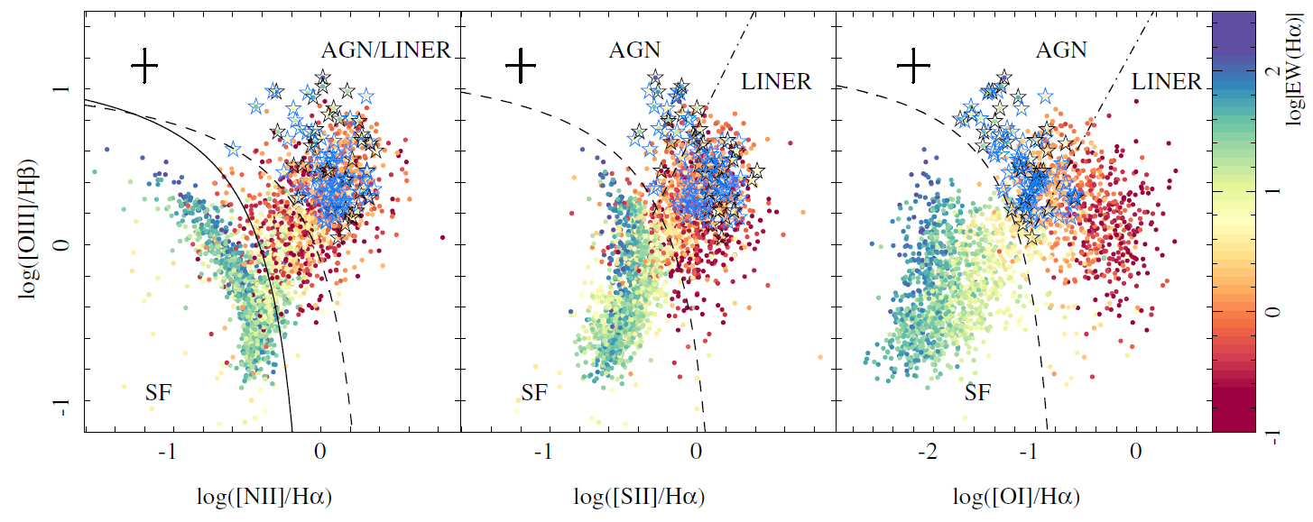
Fig. 1 Diagnostic diagrams for the central ionized gas of the sample galaxies, including the distributions of the [O iii/Hβ] vs. [Nii]/Hα line ratio (left panel), [Oiii/Hβ] vs. [Sii]/Hα (central panel), and [Oiii/Hβ] vs. [Oi]/Hα (right panel).
Although they are frequently used, the nature and meaning of the listed demarcation lines is largely unknown. The Kauffmann curve is a pure empirical tracing of the so-called classical location of starforming/H ii regions drawn to select the envelope of the galaxies that are supposed to form stars in the SDSS-DR1 catalog. Therefore, it is supposed to select the most secure higher envelope for star-forming regions: i.e., line ratios above that curve are unlikely to be produced by ionization by young stars. However, below that curve one could still have many different sources of ionization, contrary to the common understanding of this curve. The Kewley curve is a more physically-driven envelope, derived from the analysis of the expected line ratios extracted from photoionization models where the ionizing source is a set of young stars created along a continuous starformation process over a maximum of 4 Myr (for longer times little differences were found). Thus, this demarcation line indicates that line ratios above it cannot be produced by ionization by young stars (within the assumptions of the considered models). However, it says nothing regarding the nature of the ionization below it, again, contrary to the common understanding of this curve. Therefore, both lines could be used to segregate the nature of the ionization only to first order, and in the following way: above the Kauffmann (Kewley) demarcation line the ionization is unlikely (impossible) to be produced by young stars.
In summary, to consider that all ionized regions below either the Kauffmann or Kewley demarcation lines are due to photoionization associated with OB stars is a frequent mistake. Indeed, it is clearly appreciated that below both curves, and in particular the Kewley one, there is a large number of ionized regions with equivalent widths well below 6ºA (Figure 1, left panel), a limit introduced by Sánchez et al. (2014) to impose the minimum contribution of young stars to explain the observed ionization. This limit has been recently confirmed using photoionization models by Morisset et al. (2016). However, it is true that most of the ionized regions below this demarcation lines (and in particular the Kauffmann one) present larger EWs, and are compatible with ionization associated with star-forming regions. On the other hand, most of the regions above the considered demarcation lines present equivalent widths of Hα below 3ºA (and of the order of ≈1-2ºA), in particular above the Kewley curve. These values are the typical ones observed in ionization due to post-AGBs (e.g. Binette et al. 1994; Stasin ́ska et al. 2008; Sarzi et al. 2010; Papaderos et al. 2013; Gomes et al. 2016a; Morisset et al. 2016). It may be that there are still weak AGNs that show low equivalent widths, but by construction they are indistinguishable from ionization due to the old stellar component, based only on the information provided by optical spectroscopy.
Contrary to common expectation, the ionization due to post-AGB stars is not only located above the described demarcation lines, but it is frequently found in the bottom-right end of the classical location of Hii regions, extending to the area normally associated with the LINER-like emission (e.g. Gomes et al. 2016b; Morisset et al. 2016). Finally, other sources of ionization, like shocks, are distributed well below and above the two demarcation lines. Therefore, they are in essence useless to distinguish the source of ionization in this regards unless they are combined with other information, like the morphology of the ionized area or its kinematics (e.g., Wild et al. 2014; López-Cobá et al. 2017).
3.5.1. The AGN Selection Procedure
In accordance to the discussion above, to select our AGN candidates we apply a double criterion, imposing that (i) they have emission line ratios above the Kewley demarcation line (i.e., we exclude the star-forming regions) and (ii) the EW(Hα) is larger than 1.5ºA in the central regions, following Cid Fernandes et al. (2010), but relaxing the criterion to include weaker AGNs.
Based on the three diagnostic diagrams shown in Figure 1 we find 683 galaxies with its central ionization above the Kewley curve in the first panel ([Nii]/Hα). Out of them 142 have an equivalent width larger than 1.5ºA. For those 683 galaxies, 629 are above the Kewley demarcation line for the central panel ([S ii]/Hα), with 125 fulfilling the EW criterion. Finally, of those 629 only 302 are above the demarcation line for the right panel ([O i]/Hα), with 97 fulfilling the EW criterion. Those ones represent the final sample of AGN candidates; they are labeled as open stars in Figure 1. It is worth noticing that our selected candidates are mostly above the Seyfert/LINER demarcation line for the [O I]/Hα diagram (with only 11 out of 97 objects below that curve). However, our selection still excludes one fourth of the objects above that demarcation line. This diagram presents a more clear bi-modality in the distribution of points, with a better segregation in terms of the EW(Hα) for galaxies above and below the Kewley demarcation line. This is clear evidence that [OI]/Hα is a much better tracer of the ionization strength than the other two line ratios (e.g. Schawinski et al. 2010). On the other hand, our selection criteria disagree completely with the Seyfert/LINER demarcation line proposed for the [N ii]/Hα and [S ii]/Hα diagnostic diagrams (as can be appreciated also in Schawinski et al. 2010).
3.5.2. Type-I AGNs
The most broadly accepted classification for AGNs separates them between Type-I and Type-II depending on the presence of a broad (FWHM≈1000-10000 km/s) component in the permitted emission lines (e.g. Peterson et al. 2004). The broad component is explained within the classical Unification Scheme by the existence of ionized gas close to the accretion disk of the SMBH, which moves fast on chaotic orbits due to the strong gravitational potential of the nucleus. This is the BLR region. The absence of broad forbidden lines is explained by the high density of the ionized gas. The classical explanation for the distinction between Type-I (with an observed broad component) and Type-II (without it), is the presence of a dense dust torus between this BLR and the region emitting the forbidden lines (less dense, far away and moving slowly from the nucleus) the so-called NLR, since the line-of-sight of the nucleus should be independent of it (Urry & Padovani 1995).
The selection of Type-I AGNs is based on the presence of a broad component in Hα (the permitted line strongest and easiest to analyze in our wavelength range). To do so, we fitted the stellarsubtracted spectrum in the central region of each galaxy within the wavelength range covered by Hα and the [Nii] doublet by using four Gaussian functions: three narrow ones for each nitrogen line and Hα (FWHM<250 km/s), and an additional broad component for Hα (1000<FWHM<10,000 km/s). No component is considered for the continuum emission by the AGN itself, since it is not relevant for this analysis. In a follow-up study (Cortes et al., in prep.) we are exploring in detail the properties of the Type-I AGNs themselves. There we include different models for the AGN continuum emission. The fit was performed using FIT3D (Sánchez et al. 2016b). Type-I AGN candidates were selected as objects for which the peak-intensity of the broadcomponent had a signal-to-noise larger than five. A total of 36 candidates were selected. 35 out of 36 were already selected as AGNs based on the diagnostic diagram criteria described in the previous section. The remaining one (manga-8132-6101) does not fulfill the EW cut for the narrow component, but it is above the three demarcation lines indicated before.
Our definition of Type-I AGNs is broader than the more detailed classifications commonly used in the literature, in which there is a wide range of types between Type-II and Type-I, depending on the relative strength of the narrow and broad components. Here we consider as Type-I any AGN with the presence of a detectable broad component, irrespective of its relative strength.
3.5.3. The Final Sample of AGN Galaxies
In summary, we selected 98 AGNs out of 2755 galaxies (≈4%), a fraction very similar to the one reported by Schawinski et al. (2010). For 36 of them we detected a possible broad component in the permitted lines; they were classified as Type-I AGNs (blackopen stars in Figure 1). The remaining (63AGNs) were classified as Type-II (light blue-open stars in Figure 1). Table 3 in Appendix A.2 presents the list of the AGN candidates, including the main properties used to classify them.
We should stress here that our selection is clearly biased towards gas rich, bright nuclear sources, such as any sample of optically selected AGNs. Other active nuclei like (i) the radio-galaxies, which in many cases present weak or no emission lines (e.g. Willott et al. 2001), (ii) the infrequent BL Lac or Type-0 objects (e.g. Urry & Padovani 1995), or (iii) the dusty/obscured AGNs (e.g. Benn et al. 1998) are excluded by the current selection. However, we consider that this selection does not impose any strong bias in our sample for the final goals of this study. First, the time scales between radio emission and nuclear activity in radio-loud AGNs are different, in particular for those radio-galaxies without signatures of AGN activity and extremely large radio structures (Buttiglione et al. 2010; Tadhunter et al. 2012). Therefore, they could be considered as the fossils of a past nuclear activity rather than an on-going one. Second, the number of exotic Type-O objects is so low that excluding them would not compromise our results; and third, the fraction of obscured AGNs is known to be lower than anticipated in the past, and there are few differences in the selection of optical and X-ray AGNs apart from the range of weak AGNs, that in any case is excluded from our analysis (e.g. Georgantopoulos & Akylas 2010). Thus, our selection is restricted to galaxies currently hosting an active and strong AGN with enough gas to present clear signatures of the activity in the optical emission lines.
4. Results
4.1. Which Galaxies Host an AGN?
Figure 2 shows the morphological distribution of the AGN hosts (Type-II and Type-I), compared to that of their non-active counterparts, according to different properties of those galaxies: (i) the integrated stellar mass, (ii) the Sersic index, (iii) the stellar mass density in the central region, and (iv) the rotation velocity-to-velocity dispersion ratio (v/σ) within one effective radius. The general trends found for the bulk of galaxies among their morphological type and the different analyzed properties follow on average the expected distributions. Latetype galaxies are in general less massive, less concentrated (lower Sersic indices), have smaller central stellar mass densities, and are more frequently supported by rotation than by pressure (disordered motions). On the other hand, early-type galaxies are more massive, more concentrated, have larger stellar mass densities, and are more frequently supported by pressure. The trends are clearly defined for all morphological types, in agreement with previous results based on larger statistical samples (e.g. Nair & Abraham 2010). Only for the elliptical galaxies (E-type) we find a slightly wider distribution of the analyzed properties, in particular for the V/σ ratio. Furthermore, there is a clear trend of the morphology of the galaxies and the Hα EW in the central regions, with late-type galaxies presenting higher values than early-type ones, most likely as a consequence of the connection between morphology and ionization in galaxies.
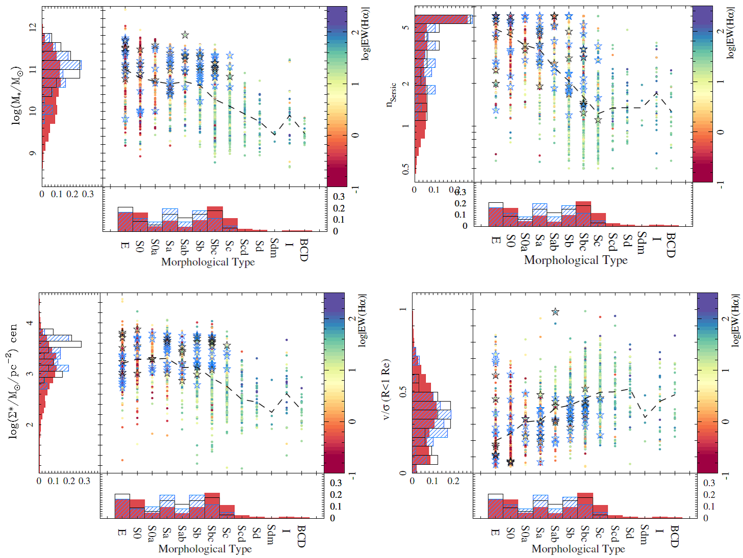
Fig. 2 Distribution of stellar masses (top-left panel), Sersic indices (top-right panel), central stellar mass density (bottom-left panel) and v/σ ratio within one effective radius (bottom-right panel) versus morphological type for the full sample of galaxies.
Regarding stellar mass, AGN galaxies, especially Type-I, present a distribution strongly biased toward larger masses compared to the distribution of non-active ones (see first panel in Figure 2). For the morphology, the fraction of elliptical galaxies is rather similar for non-active, Type-I and TypeII AGN galaxies, indicating no clear preference for AGNs to be located in these types of galaxies. For lenticular galaxies, there is a deficit of both AGN types in comparison with E-type or Sa galaxies. Type-II AGNs are more frequently found in earlytype spirals. In particular, the fraction of these objects found in S0a, Sa and Sab is almost twice than that of their non-active counterparts, at the expense of a much lower number in Sbc, None of them occur in later type spirals. Type-I AGNs are found also in early-type spirals. However, they are far more frequent in Sb and Sbc galaxies. Taking into account that our morphological classification for Type-I AGNs maybe affected by the presence of the point-like source itself we will take that distinction between both types with caution. In spite of this caveat, in general we can conclude that the morphological distribution of AGN hosts compared to that of non-active galaxies is biased toward types S0a-Sbc (≈70%) and E/S0 (≈30%) and none occur in spirals later than Sc. A similar result was previously reported (e.g., Catalán-Torrecilla et al. 2017).
Regarding the presence of bars, we find that ≈50% of the spiral AGN hosts do not present evidence of bars. This fraction is clearly lower than the value found for all the galaxies (≈70%, see e.g. Menéndez-Delmestre et al. 2007; Sheth et al. 2008; Cisternas et al. 2015). Indeed, AGN hosts show a larger fraction of strong bars (≈40%) and a similar fraction of weak bars. This result may indicate that AGNs are more frequently found in barred galaxies, a result that it is controversial, since different authors have found different results (e.g. Cisternas et al. 2015). However, we have to take it with caution. The detectability of a bar is affected by many parameters, from the selected observed band to the resolution of the images. Considering the wide range of redshifts covered by the MaNGA sample we cannot be totally sure that our detectability is not affected by resolution effects. Furthermore, AGN hosts are biased towards earlier-type spirals in our sample, and in this regime the fraction of barred galaxies increases. A more detailed analysis of the bar fraction on a sub-set of well resolved galaxies will be presented elsewhere (Hernandez-Toledo et al., in prep.)
In Figure 2 we represent with a dashed-line the mean value of the considered parameter for each morphological type. The location of AGN hosts (represented by open stars) is clearly asymmetrical with respect to this mean value. In general, they are more massive (≈75% above the mean value), more concentrated (≈70%), have larger stellar-mass densities in the central regions (≈75%), and are less rotationalsupported (≈65%). Moreover, like in the case of the morphological distribution, we find clear differences between Type-I and Type-II AGNs. The former are more massive in general (≈84%), with higher mass densities in the central regions (≈79%), and more dominated by pressure (≈80%).
4.2. Are AGN Hosts in the Green Valley?
During the last decade it has been clearly established that galaxies in the Local Universe and at least in the last ≈8-9 Gyrs (z ≈1) present a clear bimodality in most of their properties (Strateva et al. 2001; Baldry et al. 2004; Blanton et al. 2003; Bell et al. 2004; Blanton et al. 2005, for a review, see Blanton & Moustakas 2009). On one hand, earlytype galaxies are mostly supported by velocity dispersion, they are more compact, more massive, and are populated by older stars. They have lower gas fractions, and a lower degree or almost absence of SF. On the other hand, late-type galaxies are mostly supported by rotation, are less compact, less massive, and have younger stellar populations. They also present higher gas fractions, and a larger degree of SF. This separation by their main properties does not show as a continuous distribution, but it has a bimodal shape. This is evident when most of those properties are compared, and it was first highlighted in the CMDs. When integrated blue-to-red colors of galaxies are represented along their absolute magnitude, earlyand late-type galaxies split clearly into two groups: (i) the red sequence (already known for decades from the study of galaxy clusters, e.g. Butcher & Oemler 1984; Sánchez & GonzálezSerrano 2002; Sánchez et al. 2007b) and (ii) the blue cloud. In between, there is a region with a small number density of galaxies, frequently known as the green valley, GV. This bimodal distribution and the scarcity of galaxies in the GV suggest that the transformation (if any) between both groups has to be fast compared with the Hubble time (e.g., Bell et al. 2004; Faber et al. 2007; Martin et al. 2007; Gonçalves et al. 2012; Lian et al. 2016, but see Schawinski et al. 2014 and Smethurst et al. 2015). The fact that galaxies in low density groups, strongly affected by tidal interactions and with signatures of E+A spectra, are more frequently found in the GV (e.g. Bitsakis et al. 2016) supports the scenario that these are galaxies undergoing transformation.
Negative feedback produced by AGN has been proposed as a mechanism for halting SF (see references in the Introduction), and hence, for fostering the transition from the blue cloud to the red sequence (e.g. Catalán-Torrecilla et al. 2017). The fact that AGN hosts are mostly located in the transitory GV region supports this proposal (e.g. Kauffmann et al. 2003a; Sánchez et al. 2004b, but see Xue et al. 2010 and Trump et al. 2015). Following, we will explore whether the AGN host galaxies in the MaNGA sample are in the GV or not.
4.2.1. Color-Magnitude Diagram
Figure 3, left panel, shows the u − i vs. Mabs,i CMD for the full sample of galaxies, together with the AGN hosts. The magnitudes have been extracted from the MaNGA datacubes, co-adding the spectra within the FoV, convolving them with the transmission of the considered SDSS filters, and deriving the magnitudes in the AB photometric system. There is a clear bimodal distribution in the CMD, better highlighted by the typical EW of Hα in the central regions of the galaxies: galaxies in the red sequence present a low EW of Hα in most of the cases (≈1-3ºA), while galaxies in the blue cloud present much larger values (≈10-500ºA). AGN hosts are mostly located in the bluer end of the redsequence towards the GV. This is also evident in the color histograms of the same figure. In general TypeII AGNs are more clearly packed just below the red sequence, covering a narrower range of colors. On the other hand, Type-I ones are distributed covering a broader range of colors. This very same result was already noticed by Sánchez et al. (2004b).
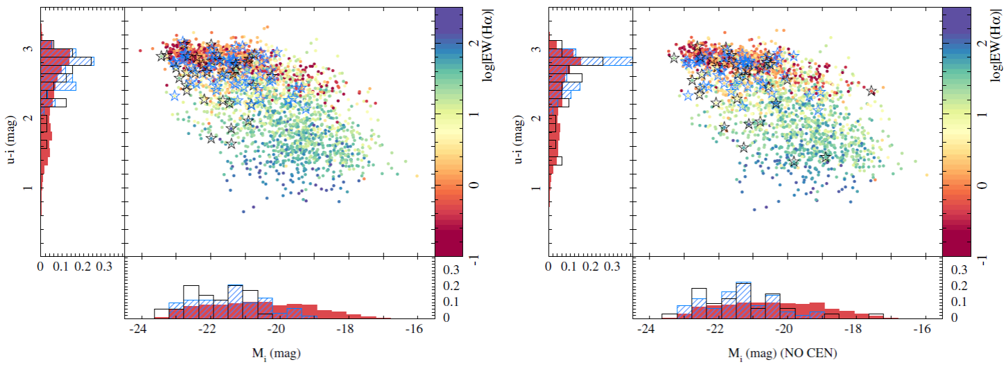
Fig. 3 Distribution of u − i color versus i-band absolute magnitude (CMD) for the full sample of galaxies analyzed in this study, using the same symbols as in Figure 1.
A basic criticism to the described location of AGN hosts in the CMD is that the nuclear source, intrinsically blue and potentially strong, may alter the overall colors of the objects and shift them towards the GV. This could be particularly important in the case of Type-I AGNs (e.g. Sánchez & González-Serrano 2003; Jahnke et al. 2004a,b; Zhang et al. 2016). In order to explore that possibility we have repeated the derivation of the magnitudes and colors but subtracting the central spectra for each datacube. The central spectra correspond roughly to an aperture of the size of the PSF, and in principle should remove the strongest effects of the nuclear source. This procedure was performed for all the galaxies, irrespective of the presence or not of an AGN. Figure 3, right panel, shows the CMD for the full sample of galaxies and the AGN hosts once this nuclear subtraction was performed. Despite having subtracted the nuclear region, the new distribution looks very similar to the previous one. The colors of Type-II AGN hosts are more concentrated towards the region just below the red sequence, as is clearly seen when comparing their histograms. Type-I hosts appear more dispersed, occupying the GV region. For some particular objects the contamination by the AGN is very strong, in particular for Type-I hosts. In at least three cases they shift to very different locations from the initial ones, moving from the red sequence to the blue cloud (two cases) or towards the lower luminosity end of that sequence (one case). However, this does not affect the overall distribution.
This result indicates that most of AGN hosts are really located in the intermediate region between the blue cloud and the red sequence, and this preferential location does not seem to be induced by the photometric pollution of the AGN itself.
4.2.2. Star Formation vs. Stellar Mass
The location of AGN hosts in the GV of the CMD has induced other authors to explore whether they are located also in intermediate positions of other diagrams that exhibit a bimodal distribution. A major example is the SFR vs. integrated stellar mass diagram (Brinchmann et al. 2004; Salim et al. 2007; Noeske et al. 2007; Renzini & Peng 2015; Sparre et al. 2015, etc). This diagram shows two clearly distinct regions where galaxies concentrate (e.g., CanoDíaz et al. 2016): (i) the star-forming main sequence (SFMS), which shows a linear correlation between the logarithm of the SFR and the logarithm of M, with a slope slightly less than one (≈0.8), and (ii) the sequence of passive or retired galaxies, RGs, which shows another linear correlation but with a smaller normalization and a slope slightly larger than that of SFMS. Both correlations exhibit a tight distribution, with a dispersion of ≈0.2-0.3 dex, slightly larger in the case of the RGs. The slope of the SFMS seems to be rather constant over cosmological time. However, the zero-point presents a shift towards larger values in the past, following the cosmological evolution of the SFR in the Universe (see Speagle et al. 2014, Katsianis et al. 2015, and Rodríguez-Puebla et al. 2017 for a recent compilation of many works).
The nature of these correlations is intrinsically different, and it usually generates some confusion. The former correlation indicates that when galaxies form stars, the integrated SFR follows a power of the look-back time (not an exponential profile as generally assumed), with the power being almost constant in at least the last 8 Gyrs. The later correlation does not reflect any kind of connection between the SFR and M, since actually the dominant ionizing source for galaxies in the RG sequence is not compatible with SF. As pointed out by Cano-Díaz et al. (2016), their ionization is located in the so-called LINER-like (or LIER) area of the BPT diagram, and is most probably dominated by some source of ionization produced by old-stars (e.g., post-AGBs; Keel 1983; Binette et al. 1994, 2009; Sarzi et al. 2010; Cid Fernandes et al. 2011; Papaderos et al. 2013; Singh et al. 2013; Gomes et al. 2016a,b; Belfiore et al. 2017). The fact that its luminosity correlates with M reinforces its stellar nature, indicating that it most probably presents a characteristic EW(Hα) (e.g. Morisset et al. 2016). Actually, when the SFR is not derived from the Hα ionized gas, like in our case, but is extracted from the analysis of the stellar population using inversion methods, this second trend is less evident, as pointed out by González Delgado et al. (2017).
Figure 4 shows the SFR-M diagram for the full sample of galaxies analyzed here, together with the AGNs hosts. The well known bi-modal distribution is highlighted by the clear difference between the EW of Hα in the central regions between the SFMS and the RG sequence, with a segregation more pronounced than in the case of the CMD. Actually, Cano-Diaz et al. (in prep.) have shown that by making a cut at the EW(Hα)=6ºA it is possible to distinguish clearly not only between the SFMS and RGs but between star-forming and non star-forming regions within the galaxies. We will use this criterion to define star-forming/non star-forming regions and galaxies through this study.
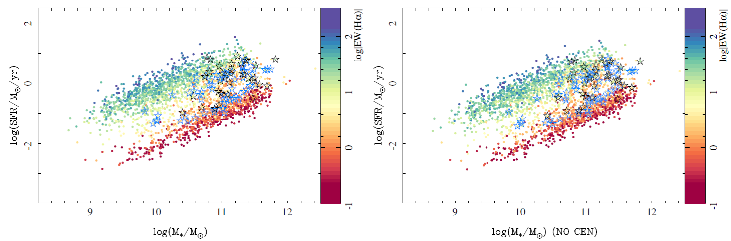
Fig. 4 Distribution of the SFR versus the stellar mass for the full sample of galaxies analyzed in this study, using the same symbols as in Figure 1. We should note that the SFR, as defined here, is just a linear transformation of the Hα luminosity, and for RGs it should be considered as an upper-limit to the real SFR (due to the contribution of other ionization sources).
The location of the AGN hosts between the regions of the SFMS and the RGs sequence in the SFR- M *diagram was first reported by Cano-Díaz et al. (2016), already hinted at by Catalán-Torrecilla et al. (2015) and confirmed by Catalán-Torrecilla et al. (2017). Figure 4 confirms these results. Both TypeI and Type-II AGN hosts are clearly located between the SFMS and RG regions. Like in the case of the CMD, the location of both AGN types is slightly different. Type-I hosts are more concentrated in the higher-mass range and more frequently found in the lower end of the SFMS. On the other hand, Type-II hosts are more broadly distributed in terms of their mass (also seen in Figure 2, upper-left panel), and they are found both in the lower-end of the SFMS and the upper-end of the RGs region. We cannot envision any non-physical reason or selection bias that explains this separation. If true, it may indicate that both families of AGNs are intrinsically different, or at least that they host galaxies that evolve in a different way.
As in the case of the CMD, a possible reason why AGN hosts are located in the intermediate regions between star-forming and non star-forming galaxies could be the contamination of the nuclear source. In this particular case the strongest effect would be an increase of the Hα luminosity, due to ionization by the AGN, which will shift galaxies in the RG sequence up towards the intermediate area. CatalánTorrecilla et al. (2015) already explored that possibility for Type-II AGNs and found that the contamination is small and can be neglected in comparison with the overall integrated Hα luminosity across the entire galaxy. This has not been tested yet for Type-I AGNs. Despite the possible contamination by the central ionization through the entire optical extension of the host galaxy that has been observed in different AGNs (e.g. Husemann et al. 2010; GarcíaLorenzo et al. 2005a), the strongest contribution is located in the central regions. Therefore, following the same procedure described for the CMD above, we estimate the decontaminated stellar-mass density and SFR by subtracting the contribution of the central region (PSF size) to both quantities. Figure 4, right-panel, shows the result of this analysis. As in the case of the CMD, and in agreement with the results from Catalán-Torrecilla et al. (2015) and Catalán-Torrecilla et al. (2017), the location within the SFR-M diagram of AGN hosts is not significantly affected by the possible pollution by the nuclear source. This result indicates that indeed the AGNs are hosted by galaxies that are genuinely located in the intermediate/transition region between the SFMS and the RG regions in the SFR-M diagram.
It is still possible that the selected AGN hosts are located in the GV due to poor selection. As we stated in § 3.5.3 our selection excludes weak AGNs that may reside in early-type, gas poor and mostly retired galaxies; in particular, we have excluded all radio-galaxies. Those AGNs would reside most probably in the sequence of RGs. However, as stated before, the time-scales between the extended radio emission and the nuclear activity may be different, with the former being much longer, and here we are discussing the properties of the host galaxies of currently active AGNs. While most of the radioloud but optically inactive galaxies would reside in the RG region (e.g., M87 Butcher et al. 1980), we speculate that the optically active ones - those that present strong optical emission lines (e.g., 3C120 Sánchez et al. 2004a; García-Lorenzo et al. 2005b) - should be located in the GV as their radio-quiet counter parts. We intend to explore this possibility in a future study.
On the other hand, our optically selected AGN candidates may be out-shined by the intense circumnuclear SF in the case of the bright star-forming galaxies. Ellison et al. (2018) have recently confirmed that galaxies with stronger integrated SFR are those that present stronger nuclear ΣSFR compared to the average population. Based on this result it may be possible that our AGN detection is precluded for galaxies in the SFMS, and, in combination with our bias against gas poor/weak AGNs, we will detect only those found in the GV due to poor selection. We explore that possibility by comparing the Hα flux intensities and luminosities with the central aperture considered in this study between active and non-active galaxies. While we reproduce the results of Ellison et al. (2018), none of the SF galaxies has an Hα luminosity stronger than the selected AGNs. Thus, being out-shined by a circumnuclear SF is highly unlikely. It is even more unlikely if we consider that due to the strong differences in the line ratios an AGN would present clear signatures in the emission line ratios even if the Hα luminosity were 10 times weaker than that produced by SF in the same aperture. We should stress here that this holds for kpc-scale spatially resolved spectroscopic data. In the case of flux intensities integrated over much larger apertures, in particular for the full optical extension of the galaxies, the shading by SF should have a stronger effect.
4.2.3. The Age-Mass Diagram
Within most of the proposed scenarios, galaxies in the GV (like AGN hosts) are in transition between the SFMS and RG region. It is possible to estimate the amount of time required to complete the transition by comparing the average ages of the stellar populations for the SFGs, RGs, and AGN hosts. Figure 5 shows the characteristic luminosity and mass weighted ages for the stellar populations (i.e., the value at the effective radius, González Delgado et al. 2016; Sánchez et al. 2016a) for all the analyzed galaxies, together with the AGN hosts. Like in the case of the CMD and the SFR-M diagram, AGN hosts are located in an intermediate region between the intermediate/young-age SFGs and the old RGs. For the luminosity-weighted ages (normalized at 5500A,¡ Sánchez et al. 2016b), which are more sensitive to the young stellar populations, the AGN hosts are ≈3 Gyr older than the SFGs and ≈3 Gyr younger than the RGs. In the case of the mass-weighted ages, which are more sensitive to the bulk of stars on average formed at early cosmological times (e.g. PérezGonzález et al. 2008; Pérez et al. 2013; Ibarra-Medel et al. 2016), the respective differences are of ≈1 Gyr compared to the RGs and ≈2 Gyr compared to the SFGs. If we consider the offsets between the average ages for the different types of galaxies as a clock for the last massive SF event that contributed significantly to the light (and in lesser amount to the mass of the galaxy) we may consider that the quenching in local AGN hosts happened about 1-2 Gyrs ago.
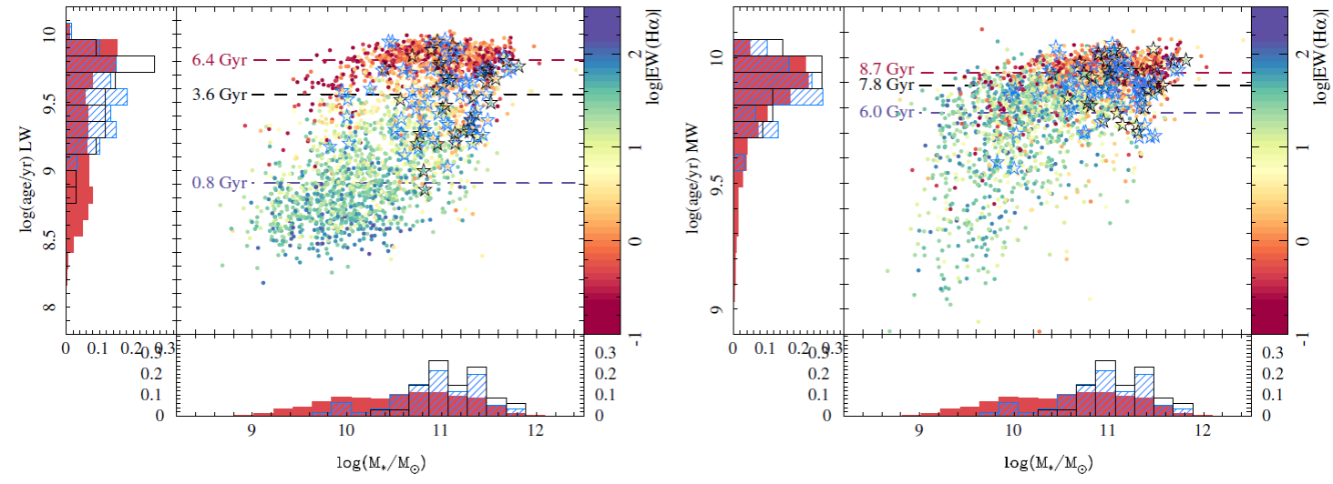
Fig. 5 Distribution of the average age along the stellar mass for the full sample of galaxies analyzed in this study, using the same symbols as horizontal lines and the corresponding values indicate the average ages for the RGs (red), AGNs (black) and SFGs (purple). The color _gure can be viewed online.
Despite these results, we should be cautious in making a causal connection between AGN activity and the transition between both groups. In particular, we should highlight the fact that only one-half to one-third of the galaxies in the so-called GV (either in the CMD or the SFR-M∗ diagrams) host an AGN. For the remaining galaxies, either the AGN is too weak to be selected by the restrictive EW cut or they do not host a nuclear source, and therefore, their transition either implies a different time-scale than the AGN activity or there is no mandatory need for an AGN to be active during the transition process. We should keep that in mind in order not to over-interpret the results.
Finally, more recent studies have suggested that the preference of AGNs for the GV and bulgedominated galaxies is the result of selection effects (see e.g., Xue et al. 2010; Trump et al. 2015, and references therein). A selection effect could be due to the fact that AGN signatures in the diagnostic diagrams can be hidden by Hii regions in galaxies with significant levels of SF, particularly in the BPT diagram, and after accounting for this bias AGNs are most common in massive galaxies with high sSFRs (Trump et al. 2015). Note, however, that this is not applicable to our analysis since we are using a more restrictive criterion for selecting AGNs, which results in a selection of strong AGNs. Indeed, strong AGNs are expected to affect more their host galaxies. Moreover, it is not clear whether the above mentioned studies could have aperture effects on their AGN detections, which is not our case.
4.3. Metal Content in AGN Hosts
Based on the previous results we cannot determine if AGN hosts are in a transition from the SFMS towards the RG sequence (or from the blue cloud to the red sequence), or the other way around. Alternative scenarios involve a rejuvenation of already RGs by accretion of gas or capture/minor-merger with gas rich galaxies (e.g., Thomas et al. 2010). Actually, early-type galaxies with blue colors, recent SF activity, and even with faint spiral-like structures, have been previously detected (Schawinski et al. 2009; Kannappan et al. 2009; Thomas et al. 2010; McIntosh et al. 2014; Schawinski et al. 2014; Vulcani et al. 2015; Lacerna et al. 2016; Gomes et al. 2016b). The fraction of these galaxies increases as the mass decreases and the environment is less dense. A new gas fueling could activate the nuclear AGN too, increasing slightly the SFR and could make the colors bluer; we will equally detect the host galaxy in the green valley.
A possible way of distinguishing between these two scenarios is to explore the metal content in these galaxies. If the SF is quenched at a certain time, when the AGN is still observable (i.e., within the last 108 yr, the supposed timescale of an AGN), the oxygen abundance should be “frozen”, since this is only increased by the production of short-lived massive stars that evolve into supernovae of Type-II. A similar effect could be produced by a rejuvenation if the accreted gas is less metal rich (e.g., if the captured gas-rich galaxy is less massive than the host). If the rejuvenation is due to gas that has been recycled in the host, then no decrease of the oxygen abundance is expected. This scenario for the gas-phase oxygen abundance is different from the one expected for the stellar metallicity ([Z/H]). This parameter results from the combination of the two major groups of elements produced in stars: α (like O, Mg...) and non-α elements (like Ti, Fe...). The non-α elements are produced in stars of any mass, its bulk production being dominated by intermediate mass stars, and therefore then require a longer period of time to be produced (as the stars last longer times at lower masses). If no new SF process happens, the stellar metallicity gets frozen too, since it measures the metals trapped in the stars. Therefore, in the case of a quenching of the SF both the oxygen abundance and the stellar metallicity should be lower than that of the average population of galaxies in the same mass range. However, for the rejuvenation, although the oxygen abundance may be lower (at least in some cases), the stellar metallicity should not be substantially modified. These events do not imply a SF process large enough to modify the average metallicity in a galaxy dominated by the bulk of stars formed in early times (Pérez et al. 2013; Ibarra-Medel et al. 2016), since they involve just a tiny fraction of the overall stellar mass. Therefore, it is expected that they do not modify the stellar metallicity.
Figure 6, left panel, shows the central massweighted stellar metallicity versus the integrated stellar mass for all the galaxies explored in this analysis, together with the distribution for AGN hosts. There is a clear correlation between both parameters, known as the stellar mass-metallicity relation (MZR), which in our case is well represented by the black solid line. For comparison purposes we include the MZR presented by González Delgado et al. (2014a) using IFS data from the CALIFA survey (dashed grey line). Both relations follow the same trend, with a clear offset towards lower metallicities (∆[Z/H] ≈ −0.1 dex) for the relation proposed by González Delgado et al. (2014a). This result is expected, since the library of SSPs templates adopted in that study comprises stellar populations covering a much wider metallicity range, including very metal poor populations not considered in our adopted library. Despite this offset, the general trends are pretty similar.
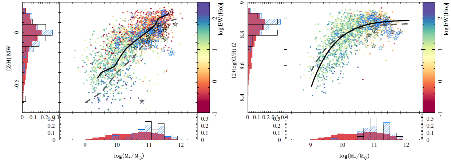
Fig. 6 Left panel: Distribution of the mass-weighted stellar metallicity within one effective radius versus the stellar mass for the full sample of galaxies analyzed in this study, using the same symbols as in Figure 1.
The location of AGN hosts in this diagram covers the more massive range, as expected from the results seen in previous sections. More interestingly, AGN hosts are preferably located below the value of the mean stellar metallicity for each mass (stellar MRZ), with 69% in the lower-metallicity range compared to 31% in the upper-metallicity one. This trend is sharper for Type-I AGN hosts, with 77% of them located in the lowermetallicity range.
Figure 6, right-panel, shows the distribution of the characteristic oxygen abundance along the integrated stellar mass for the sample of 1641 nonactive galaxies with detected emission lines compatible with being ionized by SF and enough spatial coverage to derive the abundance at the effective radius (following Sánchez et al. 2014; Sánchez-Menguiano et al. 2016; Sánchez et al. 2017; Barrera-Ballesteros et al. 2017). As indicated in § 3, we adopted the t2 calibrator for the oxygen abundance. However, no qualitative result would change if other calibrator is assumed. The average trend between the two parameters is described by the solid line, following the formalism of Sánchez et al. (2017). The dashed-line shows the relation found by Barrera-Ballesteros et al. (2017), for a similar dataset. There are some differences, most probably due to differences among the samples, since in Barrera-Ballesteros et al. (2017) the AGNs were not excluded for this particular analysis.
The location of the AGN hosts in Figure 6 has been highlighted following the same symbols as in previous figures. As in the case of the stellar MZR, the galaxies hosting a nuclear source are preferably located in the low abundance regime for their stellar mass, although their fraction is a slightly lower. 61% of AGN hosts have an abundance lower than the average corresponding to their masses. As in the case of the stellar metallicity the trend is sharper for Type-I AGNs, with 70% of them having an oxygen abundance lower than the average.
These results agree with a quenching scenario rather than with the rejuvenation one, in accord with the scenario presented by Yates & Kauffmann (2014), based on the analysis of the gas and stellar metallicities of the SDSS-DR7 dataset. However, other processes may agree with the observed distributions. For example, a major merger that does not involve a strong increase in the SFR may increase the stellar mass without significantly modifying either the stellar metallicities or the gas-phase oxygen abundance.
4.4. Gas Content: What Halts Star Formation?
Having established that most of the AGN hosts are located in the intermediate region between the blue/star-forming and the red/retired galaxies, and that most probably that transition is associated with a process that halts SF, we will explore now the possible reasons for that halting. In general, there are two major possibilities: (i) a lack of molecular gas and (ii) the presence of gas in such conditions that SF is prevented. In order to explore those possibilities we analyzed the dependence of our estimation of the molecular gas mass, described in § 3.3, on both the SFR and the integrated stellar mass.
Figure 7 shows the distribution of the integrated SFR as a function of the estimated molecular gas mass for all the galaxies studied here, together with the AGN hosts. The correlation observed between both parameters was first proposed by Schmidt (1959), and it is generally known as the SchmidtKennicutt law (e.g. Kennicutt 1998). It is a direct consequence of the fact that stars are born in dense molecular gas regions. This relation was generalized for the atomic and molecular gas densities across entire galaxies by Kennicutt (1998), showing that the SFR density depends on a power of index ≈1.4-1.5 of the neutral gas mass density. The slope of this relation can be explained based on a simple self-gravitational picture, in which the large-scale SFR is presumed to scale with the growth rate of perturbations in the gas disk (e.g. Kennicutt 1998). Despite that possible explanation, different studies have derived slopes covering a wide range of values, between 1 and 2 (e.g., Gao & Solomon 2004; Narayanan et al. 2012), and with a wide range of dispersions, ranging between ≈0.05 dex and ≈0.09 dex (e.g. Komugi et al. 2012). These differences are related to (i) the assumed IMFs for the derivation of the SFR, (ii) the conversion factor between the observed molecular transitions and the H2 molecular mass (e.g. Bolatto et al. 2013, 2017), and (iii) the selected tracer of that molecular gas (e.g., CO, HCN Gao & Solomon 2004). However, when the same IMF, tracer and conversion factor are applied similar trends are derived.
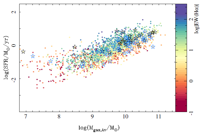
Fig. 7 Integrated SFR along the estimated integrated molecular gas mass for the full sample of galaxies analyzed in this study, using the same symbols as in Figure 1. The color figure can be viewed online.
We found a strong correlation with a coefficient r = 0.76 between the two parameters for the full sample of galaxies shown in Figure 7, with a slope less than one (α =0.62±0.02), and a dispersion σ =0.43 dex. If we restrict the analysis to the subsample of SFGs, with EW(Hα)>6ºA, the correlation is stronger (r = 0.81), the slope shifts towards a value near to one (α = 0.83 ± 0.02), and the dispersion decreases (σ =0.32 dex). This corresponds to an average depletion time of ≈4 Gyr, slightly larger than the most recently reported values (e.g. ≈2.2 Gyr, Leroy et al. 2013; Utomo et al. 2017; Colombo et al. 2017).
We must recall that our estimation of the molecular gas mass is based on an indirect calibration derived from the dust attenuation, and that for the RGs the SFR is an upper-limit at best (it is just a linear transformation from an Hα luminosity whose ionization source most probably is not young stars). In general, the distribution of SFR vs. molecular gas mass in Figure 7 is different for SFGs, defined as galaxies with EW(Hα)>6ºA, and non-SFGs (or RGs), defined as galaxies with EW(Hα)<6ºA(we use this definition for SFGs and RGs throughout this study). The former present larger SFRs at the same molecular gas mass (≈0.5 dex higher), and a larger amount of molecular gas mass (≈0.3 dex larger). This indicates that the SFGs present a global SF efficiency (SFE=SFR/Mgas) larger than the RGs. However, if we compare this distribution with those of Figure 1, 3 and 4, we do not see a clear bi-modality in this case, while SFGs and RGs are well separated in previous plots. This indicates that the Hα flux is more directly proportional to the amount of gas than to any other physical process, like the source of the ionization.
Regarding the AGN hosts, they are not distributed in any preferential region in this space of parameters, are indistinguishable for the overall population, and are not located in any transition region between SFGs and RGs (a region not clearly seen in this figure). In summary, we can conclude that if AGN hosts are forming stars they do follow a scaling relation similar to than the rest of the galaxies with respect to the available amount of molecular gas. This is consistent with the results presented by Husemann et al. (2017), where they analyze the molecular gas content in a sample of QSOs. They find that when QSOs are hosted by disk (SFG) galaxies there is no significant difference in the gas fraction. On the other hand, early-type galaxies present lower gas fractions, but shorter depletion times.
Figure 8 shows the distribution of the estimated molecular gas mass as a function of the integrated stellar mass. Over-plotted are the results of the compilation and homogenization of data from the literature recently presented by Calette et al. (2017), who were able to separate the data sets into lateand early-type galaxies and to take into account reported upper limits in the case of CO non-detections (CO is used as the main tracer of molecular hydrogen). Contrary to the SFR vs. Mgas distribution shown in Figure 7, here a clearly different pattern for SFGs and RGs is seen. A similar segregation is seen for the Calette et al. (2017) results, if we assume that most SFGs are late-type galaxies and most RGs are early-type ones. The main difference found is that the molecular gas masses for late-type galaxies in Calette et al. (2017) are smaller than the ones reported here. This could be an effect of the molecular gas estimator adopted in our study, or the result of the different selection criteria: although most of their late-type galaxies are surely SFGs, it is known that that there is no one-to-one correlation between both galaxy properties.
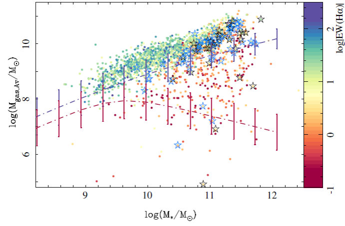
Fig. 8 Integrated molecular gas mass vs. integrated stellar mass for the same galaxies shown in Figure 7, and using the same symbols.
The SFGs in our sample present a strong (r =0.84) correlation between the two parameters, of the form:
with a dispersion σ= 0.30 dex. This means that for SFGs, the amount of molecular gas correlates tightly with the stellar mass, as reported also in Calette et al. (2017) for late-type galaxies. If we consider that the stellar mass is a good tracer of the gravitational potential within the optical extension of these galaxies, we can interpret that result as the consequence of the ability of a potential to retain a certain amount of gas if it was not previously consumed. Under this scenario SFGs form stars as fast as they can with the available amount of molecular gas (following a SK-law), and the amount of gas is somehow regulated by the potential, following a scheme similar to the one proposed in the bathtub model of Lilly et al. (2013a).
Non-star-forming (retired) galaxies present a totally different distribution. For a given integrated stellar mass, non-star-forming galaxies show a wide range of molecular gas masses that spread from an upper envelope defined by the loci of the SFGs (Equation 3) towards lower values that can be as low as 10 4M⊙ (for the galaxies with detected ionized gas, that is the majority of the galaxies in our study, § 3). This indicates that these galaxies do not form stars at the same speed as the SFGs for their corresponding stellar mass due to a general lack of molecular gas. However, it is not only the lack of gas that prevents the SF since, as we have seen when analyzing the SFR vs. Mgas distribution, those galaxies form stars at a lower efficiency than the SFGs, although that difference is less sharp than the difference found in the amount of molecular gas.
AGN hosts are found in a transition region between SFGs and RGs in Figure 8. They are located preferably at the high-mass end (which we have already seen in previous sections), mostly at the lower end of the sequence defined by the SFGs, and spread towards lower values of Mgas for a given stellar mass. The main difference between Type-I and Type-II AGNs seems to be the range of stellar masses, without a clear difference in the distribution in this diagram. Like in previous cases, we refrain from making a causal connection between the AGN activity and the process that quenched star formation.
We should note that although RGs and AGN hosts have less molecular gas and a lower SFE at the current epoch, this does not preclude having had a stronger SFE and more molecular gas in the past. Indeed, a strong star-burst process, like the one predicted by the scenario outlined by Hopkins et al. (2010), could have consumed a substantial amount of gas in the past. This does not explain the lower SFE, but it could fit the observations. We will explore the SF histories of these galaxies in future studies in order to clarify that possibility (Ibarra-Medel et al., in prep.).
4.5. Radial Distributions: Inside-Out Quenching?
In this section we explore whether the transition hinted at in previous sections happens in a homogeneous way in galaxies or if it happens from the outer to the inner parts, or the other way around. For this analysis we will consider all AGN types together in order to increase the statistical numbers in the different analyzed bins.
Figure 9, top panels, shows the azimuthally averaged radial profiles (in units of the effective radii) of the SF surface density (ΣS F R ) for the SFGs (left panel), AGN hosts (middle panel), and RGs (right panel), averaged by galaxy type in four different ranges of stellar mass. As expected, the SFGs have larger values of ΣS F R at any radius, with a clear inverse gradient following almost a pure exponential profile, with a slope of ≈1 dex/Re, similar for all stellar mass bins. On average, the ΣSFR for the less massive galaxies (M∗ ≈ 10M⊙ ) is ≈0.4 dex weaker than for the more massive ones (M∗ ≈ 10− 10M⊙ ), as a consequence of the local and global SFMS (e.g. Cano-Díaz et al. 2016). However, the most massive galaxies seem to present a slightly lower ΣS F R , which may indicate that for these galaxies the global SFR has started to deviate from the MS towards the GV, as already pointed out by different authors (e.g. Catalán-Torrecilla et al. 2015; González Delgado et al. 2016, and references therein). The RGs present a SF surface density one dex weaker than SFGs at any stellar mass range and at any galactocentric distance. Their profiles are less steep than those of the SFGs, with a shape that resembles a de Vaucouleurs (de Vaucouleurs 1959) or Sersic (Sersic 1968) profile rather than a pure exponential (Freeman 1970). The difference between the less massive and the more massive galaxies is larger than in the case of the SFGs, being of the order of ≈0.6 dex. This reflects the fact that the spatial resolved RG sequence has a steeper slope than the SFMS (Cano-Diaz et al., in prep.). Like in previous cases we must recall that the ΣS F R for the RGs should be interpreted as purely Hα luminosity densities, whose ionization nature should not be directly associated with young stars, and should be regarded as an upper limit of the real ΣSFR.
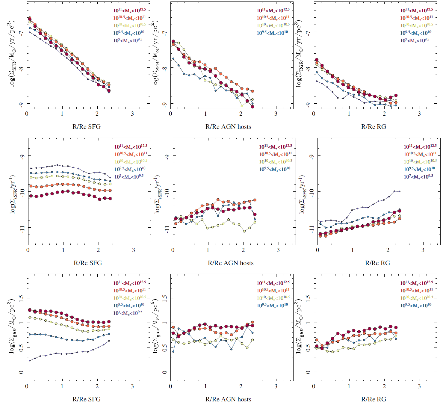
Fig. 9 From top to bottom each panel shows the radial distributions of (i) the SFR, (ii) sSFR and (iii) molecular gas surface densities for three categories of galaxies: SFGs (left panels), AGN hosts (central panels), RGs (right panels). In each panel is shown the average distribution of the considered parameter for the galaxies within four different mass bins: 107 -109.5 (dark blue), 109.5 -1010 (light blue), 1010 -1010.5 (yellow), 1010.5 -1011 (orange), and 1010(red) in solar masses, with symbol size increasing with mass. The color figure can be viewed online.
Finally, AGN hosts are where in between the SFMS and RG sequence, as expected from the results in § 4.2. Their ΣS F R values are slightly lower than those of the SFGs for any stellar mass bin and at any radial distance, reflecting the fact that they are galaxies for which the SFR is somehow halted to a certain degree. However, from these distributions we cannot establish wheter SF is stopped homogeneously in these galaxies, or if it follows a pattern of outside-in or inside-out quenching/halting. We should note that the number of AGN hosts in each mass bin is rather different, reflecting the fact that these objects are more frequently found in massive galaxies (§ 4.1). There is no AGN host in the lowest mass bin (M∗ ≈ 10M⊙ ), just three in the second bin (M∗ ≈ 109.75 M⊙ ), seven in the next one (M∗ ≈ 10M⊙ ) and a total of 54 in the most massive range (M∗ ≈ 1011.5 M⊙ ). This affects the statistical significance in the comparison between different bins.
Figure 9, second row panels, shows the average azimuthal radial distribution of the specific SFR (sSFR) for the same three galaxy types (SFGs, AGN hosts and RGs), averaged over the same stellar-mass bins as in the previous panels. In the case of the SFGs the sSFR shows a rather constant distribution for each different mass bin, with larger values for less massive galaxies than for more massive ones (≈0.6 dex). This result may indicate that the spatially resolved SFMS presents a similar slope for the different stellar mass bins, but with a slightly different zero-point (Cano-Díaz et al., in prep.). A similar result was found by González Delgado et al. (2016, see their Figure 10), when segregating their sample of galaxies in different morphological types. For RGs the picture is totally different. While the sSFR has lower values for the most massive galaxies than for the less massive ones, the distribution shows a clear positive gradient in all mass bins: the central regions form stars at a much lower rate than the outer parts when compared to the already formed stellar mass density. This result can be interpreted as a differential decrease in the current SFR compared with the historical SFR from the inner to the outer parts of the galaxy. In other words, it is a clear indication that the quenching happens from the inner to the outer regions. This agrees with the scenario in which quenching is related to internal processes in galaxies (e.g. Bundy et al. 2006).
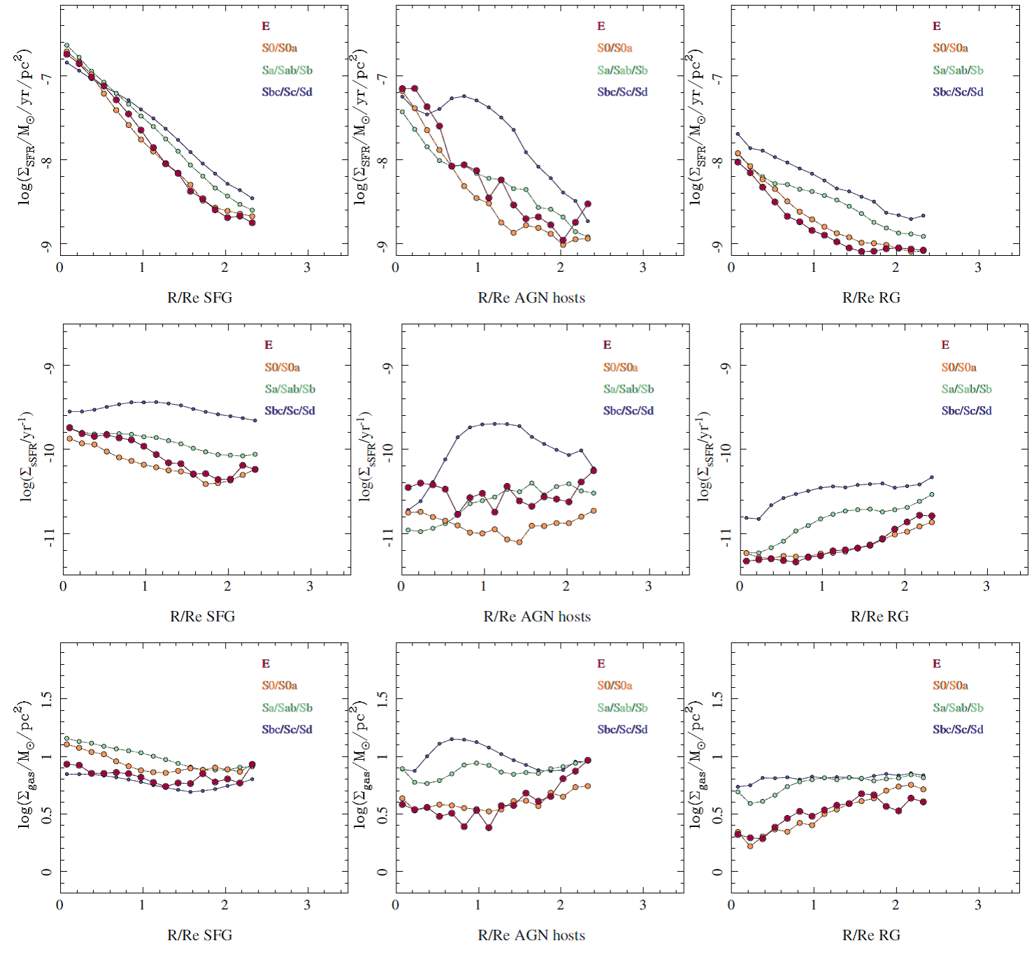
Fig. 10 From top to bottom each panel shows the radial distributions of (i) the SFR, (ii) sSFR, and (iii) molecular gas surface densities for three categories of galaxies: star-forming galaxies (left panels), AGN hosts (central panels) and retired galaxies (right panels).
Like in previous cases, AGN hosts are located in the intermediate regime between both groups of galaxies. Despite of their lower number, there are some clear differences in the radial distribution of the sSFR. Contrary to both SFGs and RGs, in AGN hosts the trend with mass is not preserved. More massive galaxies do not have a lower sSFR than less massive ones. We lack information for the lowermass bin, where we do not find AGNs. However, for the other two bins the trend is not present. Actually, the most massive and less massive bins with AGNs exhibit very similar sSFR radial distributions, with the bin in the middle showing a lower sSFR for most galactocentric distances. The limited number of galaxies in the two lowest mass bins may affect that result. In general the radial profiles are either flat or show a drop towards the inner regions (R< 1Re) with a flat distribution towards the outer ones (R> 1Re), and a mixed trend between the SFGs and RGs.
Figure 9, third row panels, shows the distribution of the azimuthally averaged molecular mass density (Σgas,Av) for different galaxy types (SFGs, AGN hosts, and RGs) and for four different mass bins. SFGs have a rather flat or positive gradient distribution in the molecular gas density for the less massive galaxies, with a value of ≈1-1.2M⊙ /pc, and a negative gradient for the remaining stellar mass bins. These latter gradients follow an almost exponential profile, with a slope clearly smaller than the one found for the ΣSFR (upper panels). The most massive galaxies show a slight drop in the Σgas,Av towards the central regions. This drop is much more evident for the RGs: for the four stellar mass bins with detected dust attenuation the inner regions show a clear deficit of molecular gas. The radial distribution has a positive non-linear gradient for undetected or nearly undetected molecular gas, several orders of magnitude lower than the values found for the SFGs at the same galactocentric distances, towards values of the same order as those of the SFGs in the outer regions (R ≈ 1.5 − 2Re). This result agrees with those presented in § 4.4, illustrating the fact that there is not only a drop in the efficiency of the SFR in these galaxies, but also a lack of molecular gas to fuel SF. Furthermore, it clearly establishes that this deficit of molecular gas is stronger in the inner regions.
Regarding AGN hosts, the lack of a similarly large number of galaxies and detected molecular gas at every galactocentric distance limits the interpretation of the results. However, despite those limitations it is clear that these galaxies exhibit a similar deficit of molecular gas, and that deficit is stronger in the inner regions. Per se this result does not support the idea of these objects being in the transition phase between SFGs and RGs. However, considering that in terms of the radial distribution of the ΣS F R and ΣsSFR these galaxies seem to be under transition, we may speculate that they first lost the molecular gas from the inner to the outer regions and than that causes the observed decrease in the absolute (SFR) and relative (sSFR) way. Since the radial distributions of Σgas,Av for AGN hosts are more similar to those of RGs while the other two radial distributions are clearly in an intermediate stage we speculate that the decrease of molecular gas in the central regions happens before that of the SFR and sSFR.
All together, AGN hosts seem to be in a transition phase between SFGs and RGs regarding the analyzed radial gradients in different mass bins.
4.6. Radial Distributions by Morphology
So far we have described the behavior of the radial profiles for different integrated stellar mass bins. Several previous studies have demonstrated that the radial properties of galaxies dependent more on morphology than on mass (e.g. Ibarra-Medel et al. 2016; González Delgado et al. 2014b,a, 2015, 2016, and references therein). Schawinski et al. (2010) found clear differences in the effects of AGNs on the evolution for different morphological types of their hosts. They propose a different transition to quiescence for early-type galaxies, that is assumed to be faster than that for late-types. We explore that possibility by comparing the radial distribution of the properties described in the previous section for different morphological-type galaxies.
Figure 10 shows the radial distributions of the same properties shown in Figure 9 (ΣSFR, ΣsSFR and Σgas,Av, in each row), for the different groups of galaxies explored in this study (SFG, AGN hosts and RG, in each column). Radial gradients in these quantities segregated by morphology have been previously studied by González Delgado et al. (2015) and González Delgado et al. (2016) using IFU data with a better physical spatial resolution than here. However, they did not split their sample into SFGs and RGs, and therefore a simple/straight-forward comparison is not possible. Regarding ΣSFR, the trends found by González Delgado et al. (2016) (their Figure 6) are very similar to the ones seen in the first row of panels of Figure 10, if we consider that most of the E/S0 galaxies are found in the RG sequence and most of the Sa-Sd galaxies in the SFMS. In general, the ΣSF R of the disk-dominated galaxies (later than Sa) shows an inverse gradient, similar to that found for SFGs at any mass bin (Figure 9, upper panels). Retired galaxies have a lower ΣS F R at any galactocentric distance and for any morphological type, apart from the later-type ones.
As in the case of the segregation by stellar mass, AGN hosts seem to be in an intermediate location between SFGs and RGs, with a ΣSFR slightly lower than that of the SFGs, and slightly larger than that of the RGs for any morphological type. Similar results are found for ΣsS F R . For any morphological type, the SFGs show a larger sSFR than those in the RGs, with the AGN hosts being in transition between the two groups. When comparing with González Delgado et al. (2016) (Figure 7), we find a slightly different shape for the radial distribution. We can reproduce their results only if we assume that most of the early-type galaxies are located in the RG sequence and most of the late-types in the SFMS. As in their case, late-type galaxies show a flatter distribution and larger values of sSFR than early-type ones for any group. However, the drop in the inner regions observed by them is only appreciated for the RGs. We find a clear difference in the shape of the sSFR for SFGs and RGs. In particular, for S0/S0a and E-type SFGs, the sSFR shows a negative gradient while the gradient tends to be positive for the RGs. For any morphological type, the transition between the SFGs and the RGs involves a drop in the sSFR from the inner to the outer regions (apart from the S0/S0a group of AGN hosts).
This result agrees with the one found for the stellar masses.
The Σgas,Av shows a similar distribution/behavior for different morphological types and different stellar masses. For SFGs, all morphological types show a shallow negative gradient, with a similar gas content in all cases. The distribution is rather different in the case of RGs, with a clear drop of molecular gas in the inner regions, which it is stronger/sharper for earlier-type galaxies than for later ones. Indeed, very little molecular gas is found in ellipticals RGs. As in previous cases, the AGN hosts seem to be in a transition regime between both groups.
A detailed analysis of the observed gradients indicates that the transition between SFG and RGs seems to happen in a different way for early-type and late-type galaxies. In the first case, the transition seems to be more abrupt (stronger change in the SFR, sSFR and gas content). In the second case, the transition is clearly smoother. This different behavior is driven by the morphology, and is not observed in the mass trends discussed in the previous section.
4.7. Non-Active Galaxies in the Green Valley
In previous sections we established that AGN hosts are located in the GV in different distributions, which highlights the bimodal distribution of the overall population of galaxies. However, it is also clear that not all galaxies in the GV host an AGN (given our detection limit and selection criteria). Thus, it is important to know if the described properties are privative of AGN hosts or if they are common to the remaining GV galaxies.
To make this comparison we need to define GV galaxies. Being an intermediate type of galaxies, located in the area of low density in either the CMD, the SFR-M or the age-mass diagrams, it is difficult to define clear boundaries to select them. In general, those limits would be somehow arbitrary and subject to fine tuning, sample completeness, refinement, or arguments regarding their selection. Following our own classification scheme, based on the distribution along the SFR-M diagram and the EW(Hα) in the central regions, we classified intermediate/GV galaxies as those galaxies whose EW(Hα) ranges between 3A and 10A. The lower limit, 3ºA corresponds to the threshold established by Cid Fernandes et al. (2010) to distinguish between RGs and SFGs, and it corresponds to the location of the 1σ upper limit of the RG sequence (Cano-Díaz et al. 2016). In a similar way, the upper-limit, 10A corresponds roughly to the 1σ lower-limit of the SFG sequence. Thus, this regime corresponds to galaxies that are at least 1σ off and in between the SFG and RG sequences. These limits are similar to the ones defined by Lacerda et al. (2018) to distinguish between DIG and SF dominated regimes. This range corresponds to the location in the SFMS diagram where a significant fraction of the AGN hosts are located. We find 220 galaxies in this GV area among the non-active galaxies (galaxies not hosting an AGN). This means that ≈1/3 of all galaxies in the GV host an AGN, a proportion clearly larger than the general fraction in the total population (≈3-4%).
Figure 11 shows the radial distributions of the same quantities shown in Figure 9, but now for the GV galaxies: the average SFR, sSFR and molecular gas mass surface density profiles. Qualitatively these galaxies show radial gradients similar to the AGN hosts, being clearly in an intermediate/transit regime when compared to SFGs and RGs: (i) they show lower ΣSFR, with a negative gradient from inside out; (ii) lower ΣsSFR, with a positive gradient, indicating that the SFR is smaller in the center than in the outer parts in relation to their stellar mass densities; and (iii) there is a deficit of molecular gas in the inner regions compared with SFGs, but with larger amounts than the ones found in RGs. However, despite these qualitative similarities, there are quantitative differences. In general, all the characteristics listed before that define them as intermediate galaxies are smoother in the non-active GV galaxies than in AGN hosts. (a) Their ΣS F R and ΣsS F R are slightly larger than those of AGN hosts for all mass bins and galactocentric distances, with shallower gradients in the sSFR. (b) the deficit of molecular gas in the inner regions is less pronounced, and they show a gas content in the outer regions similar to that of SFGs. However, their stellar populations are older on average, with a luminosity weighted (mass-weighted) age of 5.8 Gyr (8.5 Gyr) compared to the one reported in § 4.2.3 for AGN hosts: 3.6 Gyr (7.8 Gyr). In general they look as if they were in an earlier phase of the transition between the two families of galaxies regarding the SFR, sSFR, and molecular gas content. Regarding the stellar ages, though, they seem to be in a more advanced stage.
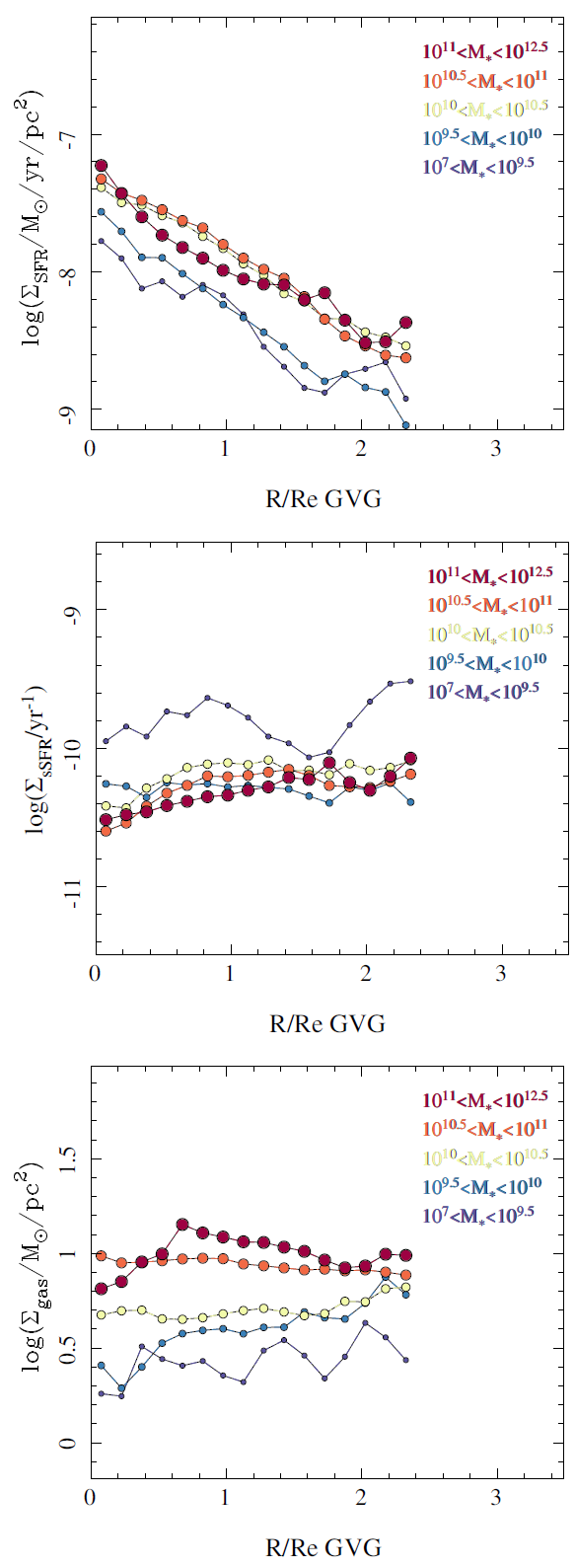
Fig. 11 From top to bottom each panel shows the radial distributions of (i) SFR, (ii) sSFR, and (iii) molecular gas surface densities for GV galaxies.
We should refrain from deriving a strong conclusion in this regard, since, as we indicated before, (i) the selection of the regime in which we classified galaxies as GV galaxies may require refinements that could affect the qualitative results, and (ii) by construction, our GV galaxies include galaxies from both our SFGs and RGs samples, and maybe we are contaminating the results. Despite all these caveats, it is clear that AGN hosts are more similar to nonactive GV galaxies than to any other family of galaxies regarding the analyzed radial distributions, and both kinds of objects show evidence of a transition between star-forming and non-star-forming galaxies, which happens from inside-out, and is associated with both a deficit of the molecular gas and decrease of the sSFR.
Figure 12 shows the radial distributions of the same properties shown in Figure 11 (ΣSF R, ΣsSF R and Σgas,Av, in each row) segregated by morphology, like in Figure 10, but for GV galaxies. In this particular case we see a clear segregation between earlyand late-type galaxies, already observed in the transition between SFGs and RGs and the AGN hosts. For the Sa to Sd galaxies, the shape of the profiles is very similar to those found for the same kind of galaxies in the RG subsample, although in general they seem to have slightly larger SFRs and sSFR, a lower decrease of the molecular gas content in the central regions, and younger stellar populations. The S0/S0a deviate from that trend in the sSFR, which shows a rise towards the inner regions, not appreciated in the RGs; they are more similar in shape to AGN hosts (Figure 10), though with slightly larger sSFR values. They also deviate in the molecular gas content, with a clearly larger amount of gas, in particular in the central regions (even when compared with AGN hosts).
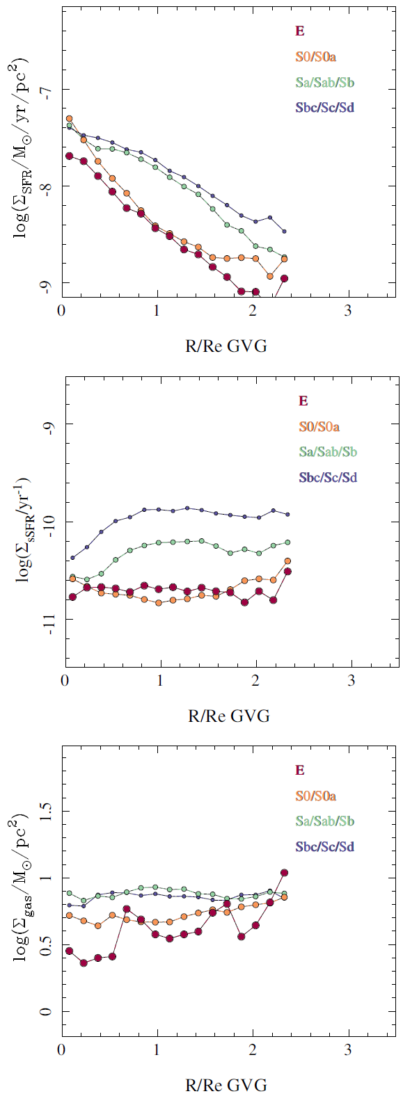
Fig. 12 From top to bottom, each panel shows the radial distributions of (i) the SFR, (ii) sSFR, and (iii) molecular gas surface densities for GV galaxies. In each panel is shown the average distribution of the considered parameter for the galaxies within four different morphological bins: Sbc/Sc/Sd (dark blue), Sa/Sab/Sb (light blue), S0/S0a (orange) and elliptical galaxies (red), with symbol size increasing for more early-type galaxies. The color figure can be viewed online.
The trends for elliptical GV galaxies are totally different from the ones present in RGs or AGN hosts with the same morphology. They show a sharper ΣSFR distribution than the RGs (as expected due to the selection criteria), but with lower SFR values than the S0 in the GV and the AGN hosts in general. Their ΣsSFR have a shallow gradient, similar to the one of the AGN hosts, but with slightly lower values. Finally, their molecular gas does not show the sharp drop in the central regions found in AGN hosts of any morphology. Their surface density is larger than that of the rest of the GV galaxies in the central regions, and similar in the outer regions. When compared with retired ellipticals is seems that there is an increase of molecular gas in the inner regions. This may indicate that these elliptical galaxies enter the GV due to rejuvenation, in particular in the central regions. Their nature seem to be different from that the AGN hosts in general. However, the small number of these galaxies (13, compared with 34-91 for the three remaining morphological groups) prevents us from making a stronger conclusion.
In summary, GV galaxies seem to be in an intermediate stage between SFG and RGs for the different morphological types. At least for non-elliptical galaxies, that transition involves a quench of the SFR and/or a deficit of molecular gas in the inner regions. However, the evident sequence appreciated when these galaxies are segregated by mass (Figure 11, § 4.7) is not present when segregating by morphology. The differences introduced by morphology are sharper, less sequential. In this regard, the apparent smooth negative gradient in the ΣSF R and shallow positive gradient in ΣsSF R seen in Figure 11 may be the result of averaging less smooth gradients over different morphologies. We will require a study with an even larger number of galaxies in order to have enough statistics to segregate non-active GV galaxies in morphology and mass bins simultaneously.
5. Discussion
Along this article we have explored the main properties of the AGN host galaxies extracted from the MaNGA survey in comparison with those of the non-nactive galaxies. We have found that optically selected AGNs are hosted by mostly early-type galaxies or early-type spirals, and that for a given morphology, their hosts are in the regime of more massive, more compact, denser central regions, and more pressure-supported than the average population of galaxies. These results seem to agree with the finding that the presence of a bulge is a mandatory condition for the presence of an active nucleus (e.g. Magorrian et al. 1998; Gebhardt et al. 2000; Häring & Rix 2004; Kormendy & Ho 2013). Our results indicate that the presence of a bulge is not only mandatory, but also the presence of a more compact, massive and dynamically hot mass concentration, more than the average at the same morphology. Despite the many caveats that can be applied to our results, in particular in the case of type-I AGNs (which disturb considerably the light-profile and therefore, the mass derivation), this result may open a new perspective in the exploration of the activation of a nuclear active region, which should be explored in the future. The activation of a SMBH into an AGN may involve/require not only the presence of a central compact object, but also the presence of a material (mainly gas) supply large enough to feed it. Different scenarios have been proposed for the AGN feeding, involving secular processes in gas rich galaxies (Hopkins & Hernquist 2009a), galaxy interactions and mergers (Sanders et al. 1988; Hopkins et al. 2006), and different kinds of instabilities (Dekel et al. 2009). However, most of them can explain only how gas is transported to the central ≈ 100−1000 pc regime.
Our results seem to indicate that whatever is the mechanism that transports gas towards the central regions, AGN activation only happens in a particular set of galaxies, those that show a larger concentration of stellar mass in the central regions, with larger disordered motions. The pro jected spatial resolution of the MaNGA IFU data, ≈2.5/FWHM, combined with the large redshift range coverage, implies that more than half of the galaxies are observed with a physical resolution between 2-4.5 kpc/FWHM. This prevents us from exploring physical conditions in the very central regions, which will require detailed observations with much a higher spatial resolution. This is a limitation of our results.
Furthermore, the segregation seems to be stronger for Type-I AGNs. They seem to be hosted more frequently by more massive, more centralconcentrated, and more pressure-supported galaxies at any morphological type. If confirmed, this result may indicate that both families of AGNs cannot be unified only by a simple inclination/line-of-sight scheme, as suggested by Urry & Padovani (1995). Other processes, like possible evolutionary steps between the two AGN types, could play a role in explaining the observed distributions (Krongold et al. 2002; Villarroel & Korn 2014)
5.1. On the Evolutionary Stage of AGN Hosts
We further discuss possible evolutionary implications from our study of the AGN hosts as compared with non-active galaxies, both regarding global properties and radial distributions. We should stress here that the possible scenarios based on our results, would have to be confirmed by larger samples and more unbiased sample selections, including both radio-loud and X-ray selected AGNs.
With regard to the loci of AGN hosts in different observational diagrams, we confirm that AGN hosts are mostly located in the so-called GV regime between the blue/SFGs and red/RGs groups, in all the different analyzed distributions: (i) the colormagnitude (or mass) diagram; (ii) the SFR-M∗ diagram; and (iii) the age-mass diagram. Indeed, onethird of the galaxies in the GV host an AGN (based on our selection criteria), while this fraction is much smaller in the SFG and RG regimes. This result is independent of the contamination of the AGN in the considered parameter. Thus, the location in the GV does not seem to be induced by a contamination by the nuclear source. This result was already suggested by several previous studies (e.g. Kauffmann et al. 2003b; Sánchez et al. 2004b; Schawinski et al. 2014), although only a few of them took into account the contamination by the central source and type-I AGNs (e.g. Sánchez et al. 2004b).
As we have indicated, galaxies show a bimodal distribution with two well separated groups of SFGs (blue, young, gas-rich, star-forming, and rotationally-supported in general) and RGs (red, old, gas-poor, non-star-forming and pressure-supported in general) for at least the last 8 Gyr (e.g. Bell et al. 2004). While stars are formed mostly in the first group (e.g. Wolf et al. 2005), the stellar mass is accumulated in the second one (e.g. Bundy et al. 2009, 2010). This implies per se that there should be a transformation from the first group (SFGs) towards the second one (RGs). That transformation requires of (1) some mass/environment-dependent evolutionary processes or the input of a large amount of energy that quenches the SF, and (2) a mechanism that transforms the morphology. The activation of an AGN (e.g. Lipari et al. 1994; Sanders & Mirabel 1996; Hopkins et al. 2009) and major mergers have been proposed to explain the first and second transforming steps, respectively. The location of AGN hosts in the transition regime between both families of galaxies seems to reinforce that scenario; the idea of having a causal connection between quenching and the ignition of the AGN activity is tempting. However, the time scales of both processes may be totally different. The best estimates of the duty cycle of an AGN indicate that most probably its activity lasts of the order of ≈0.1 Gyr (e.g., Parma et al. 2007; Shulevski et al. 2015). However, the quenching process does not seem to have a similar time scale. The age differences indicate that it can last for a few Gyr, at least when averaged across the galaxy. Therefore, rather than a causal connection we can determine that both the AGN activity and quenching happen under similar conditions in galaxies, and the former may enhance the quenching process. Another possibility is that AGNs are activated in particular periods of the quenching/transformation process. This is supported by the fact that two-thirds of the GV galaxies do not host an AGN, and by the differences in the time scales of the different processes.
There is still the possibility that the GV is populated both by galaxies in transition between SFG towards RGs or by galaxies that suffer a rejuvenation, showing a slightly younger stellar population (mostly luminosity-weighted) due to a recent ignition of the SF by the capture of either pristine gas or a gasrich satellite. However, the analysis of the location of AGN hosts in the Mass-Stellar Metallicity and Mass-gas-phase Metallicity relations (see § 4.3) suggests that this is not the main mechanism for populating the GV. Most AGN hosts show a stellar metallicity and oxygen gas abundance below the average value for their corresponding stellar mass. While the injection of more pristine gas and the ignition of SF may somehow reproduce the gas-phase abundance distribution, it can hardly modify the massweighted stellar metallicity of the galaxy, which is dominated by the old stellar population, whose bulk mass was formed long time ago in almost all galaxies (e.g. Pérez et al. 2013; Ibarra-Medel et al. 2016; González Delgado et al. 2017). The only way to decrease the stellar metallicity is that SF continues for a period at a lower rate, and that therefore there is a lack of a new population of stars more enriched than the previous one. A similar scenario was already proposed by Yates & Kauffmann (2014). At least in the case of the AGN hosts this scenario seems to be compatible with the observations.
The decrease of the SFR seems to have been primarily driven by a reduction of the available amount of molecular gas. Although we have derived just a rough estimation of this quantity, it is clear that RGs present a general deficit of gas at any mass range (§ 4.4. While SFGs exhibit a tight correlation between the integrated stellar mass and the molecular gas, RGs comprise a wide range of molecular masses, spanning from that correlation (as an upper envelope) down to several orders of magnitudes lower levels (see also Calette et al. 2017). Although this is clearly the main reason for the low SFRs in these galaxies, we have found that RGs have a SFE at least a 50% lower than SFGs for the same amount of molecular gas and stellar mass. Therefore, it is not only a lack of molecular gas that prevents/reduces the SFR but a process that inhibits SF for the same amount of molecular gas available. The lack of molecular gas could be connected somehow to the AGN activity if this is strong enough to produce outflows that expel a substantial amount of gas towards the galactic halo (e.g. Rich et al. 2010; Kraft et al. 2012; Mingo et al. 2012). However, in this case we should consider that GV galaxies without an AGN should be the remnants or fossils of previous AGN hosts. It is also possible that the decline in the SFE is related to the nuclear activity, if we consider that an AGN can inject energy that heats the gas, increasing the dispersion and preventing the formation of stars. Again, under this scenario, non-active GV galaxies should be in an evolutionary sequence towards RGs after the AGN phase(s). However, it is not clear that our results support that scenario, as we will see later.
The radial distributions of the SFR, sSFR, and molecular gas content analyzed in § 4.5 and § 4.7 agree with a scenario in which AGN hosts (and nonactive GV galaxies) are in a transition between SFGs and RGs, with a decrease/quench of the SF, at any range of stellar masses. In detail, our results indicate that the decline of the SFR happens inside-out, being stronger in the nuclear regions. This decrease is already appreciated in the most massive SFGs, which present a soft decline of the sSFR and molecular gas content in the very central regions. That decline seems to evolve towards a generalized drop of the SFR for AGN hosts, and, for the central regions, a strong decay in the sSFR and molecular gas content. Those trends are just sharper in RGs, following a clear trend. However, contrary to what we have discussed in the previous paragraph, GV galaxies do not seem to be in an evolutionary step later than AGNs in this sequence. Indeed, the analyzed radial distributions show a pattern more similar to that of the SFGs than to the RGs, with (i) ΣSFR and ΣsSFR values slightly larger than those of AGN hosts, and (ii) sSFR and molecular gas distributions with softer drops towards the inner regions. On the other hand, their ages are more similar to RGs than to AGN hosts, contrary to the previous results.
In summary, GV galaxies do not seem to fit a scheme in which they are evolving from AGN hosts towards RGs, but rather preceding active galaxies in the proposed sequence. If this is the case, then the causal connection between the ignition of the AGN activity and the quenching does not seem to fit the observations. On the contrary, if all galaxies are ordered along the considered sequence, it seems that the process that stops the SF, producing a decline of molecular gas content and a decrease of the SFE in the central regions, happens before the ignition of the AGN activity. Under this scenario, the nuclear activity may speed up the quenching process, but it does not seem to be its origin. However, there is still a third possibility, in which the quenching mechanisms for active and non-active GV galaxies are totally different and there is no evolutionary path between these two families of objects.
When analyzing the possible evolutionary paths segregating the galaxies by morphology a very similar general trend is found. Both AGN hosts and non-active GV galaxies seem to be in an intermediate step between SFGs and RGs with a general decrease of the SFR and sSFR, and a stronger decline in the sSFR and the molecular gas content in the central regions, coincident with older stellar populations. In the same way, non-active GV galaxies seem to have sSFRs and molecular gas radial distributions more similar to the SFGs than to the RGs as compared with AGN hosts. Thus, the evolutionary sequence, if it exists, indicates that the SFE and gas decline happen before the ignition of the AGN, and not after (or the two events are not causally or evolutionarily connected). The main difference with respect to the sequence described for different stellar masses is that earlyand late-type galaxies seem to present clearly distinguished evolutionary paths. Early-type galaxies show a sharper transition, in particular for non-active GV galaxies, with a larger drop in the SFR and sSFR, even with a lower or similar decline of the molecular gas content. Late-type galaxies present a lower decline in the SFR and sSFR, mostly concentrated in the central regions, e.g., SaSd GV galaxies, Figure 12 and Sbc-Sd AGN hosts, Figure 10. This result may indicate that there exists a single mechanism to explain the quenching and that bulge growth plays a role in the declining of the SFR. For bulge-dominated systems (E/S0), the decline affects the whole galaxy, while for galaxies with smaller bulges (Sa-Sd), it is clearly associated to the central regions.
The most widely accepted scenario for the transformation between late-type SFGs and early-type RGs involves a retrograde major merger between gas rich galaxies that leads to instabilities in the gas. This gas falls towards the central regions igniting a violent star-burst and producing the formation of a pressure-supported spheroid. The gas infalling to the center ignites an AGN that expels and heats the remaining gas, thus quenching the SF from the inside-out (Lipari et al. 1994; Sanders & Mirabel 1996; Hopkins & Hernquist 2009b; Hopkins et al. 2010). However, this scenario predicts that AGN hosts evolve into non-active GV galaxies as the timescale of the nuclear activity is considerably shorter than the transformation timescale. As we showed before, our results indicate the contrary: non-active GV galaxies seem to be in an earlier evolutionary stage than AGN hosts. Martig et al. (2009) proposed an alternative scenario in which the SF is halted without requiring a deficit of gas. They proposed that the growth of a stellar spheroid can stabilize the gas disk, and quench SF by preventing the fragmentation of bound gas clumps. This mechanism may fit somehow with the observed transition for late-type galaxies, and with the fact that we see a decrease of the SFE that seems to be stronger in the central regions. This scenario agrees with the recent results by Colombo et al. (2017). However, we should stress that in all the cases we observe a decrease of the gas content in those regions too, and that seems to be the primary reason of why there is no SF. Therefore, gas is expelled or consumed somehow, although the efficiency may be affected by the extra stabilization introduced by the stellar spheroid.
The questions of what produces the drop of molecular gas content in the inner regions and why the efficiency in the SF decreases remain open. The lack of molecular gas could be caused by the energy injection from the AGN itself. Outflows associated with nuclear activity are frequently found in strong AGNs (e.g. Rich et al. 2010). However, we largely ignore the effective energy input of this feedback on galaxies, despite the advances on the topic (e.g. Fabian 2012). On the other hand, central SF events may also drive outflows (e.g. López-Cobá et al. 2017), without the requirement of an AGN or a violent process. In many cases those outflows are not detected due to projection effects, and their frequency is still unclear. How much gas is expelled during this events is still under debate, although it is considered that it is proportional to the SFR (e.g. Lilly et al. 2013b), and therefore the effect should be larger in the more massive SFGs. Whether these events may be strong enough to induce an inside-out quenching that propagates through out the galaxy is unclear and dubious. In the case of the decrease of the SFE, a plausible explanation could be the scenario proposed by Martig et al. (2009). Maybe the outflows themselves trigger the creation of an spheroidal seed and the stabilization of the disk halts the SF in a more gentle way for late-type galaxies, matching the observations by Schawinski et al. (2010). This could be an scenario to be tested with simulations.
6. Conclusions
For the sample of galaxies currently observed by the MaNGA survey (DR14), we have selected AGN host galaxies based on the optical spectroscopic properties of the nuclear regions, following an spectral analysis performed using the Pipe3D pipeline (Sánchez et al. 2016a). A total of 98 AGN (36 Type-I) were selected out of ≈2700 analyzed galaxies. We have explored the main global and radial properties of these AGN galaxies and compared them with those of the non-active galaxies keeping in mind whether the galaxies are star-forming, retired or from the green valley region. Our main conclusions can be summarized in the following way:
AGN seem to be located mostly in early-type galaxies or early-type spirals. For a given morphology, AGN hosts are more frequently found in the regime of the more massive, more compact, and more pressure-supported galaxies.
AGN hosts are preferentially located in the so-called GV and intermediate regime between blue-cloud/star-forming galaxies and redsequence/retired galaxies. Their locations do not seem to be affected by the contamination from the AGN on the global properties, or by a clear bias in the selection procedure of the AGN candidates.
The population of active and non-active galaxies in the GV appears to be in a transition between SFGs towards RGs due to a decrease of the amount of molecular gas and a lower SFE. Rejuvenation, although still possible for particular galaxies, does not seem to be the main scenario to explain the properties of these galaxies.
The decline/quenching of the SFR in the evolution from the SFGs towards the RGs happens inside-out, both in AGN hosts and non-active GV galaxies. This decline seems to be primarily induced by a drop in the amount of molecular gas in the inner regions. Since our estimation of the molecular gas content is based on a dustto-gas ratio that is valid only in an statistical manner, these results should be confirmed by more direct estimations of the molecular gas, like that provided by CO measurements (e.g. Bolatto et al. 2017). Indeed, recent estimations of the molecular gas based on CO observations of MaNGA GV galaxies seem to confirm our conclusions (Lin et al. 2017).
Non-active GV galaxies do not seem to be in an evolutionary stage between AGN hosts and RGs. If there is an evolutionary sequence between these two families in the transition between SFG and RGs, non-active ones seem to be in an earlier evolutionary stage, regarding their SFR, sSFR, and gas content. That would imply that AGN activity does not seem to be the only driver for the inside-out quenching. Moreover, it may imply that there are different processes that produce the decline or quenching of the SFR. The results regarding stellar ages point towards the opposite scenario.
There is evidence of different evolutionary paths between SFGs and RGs for different morphological types. In particular, for non-active GV galaxies, the transition seems to be smoother for late-type galaxies and sharper for earlier-type ones.
In addition, we have publicly distributed all the dataproducts produced by the Pipe3D pipeline used for this work as a Value Added Catalog corresponding to the DR14 of the SDSS survey (Appendix A). To our knowledge, this is the largest distribution of this kind of IFU dataproducts produced so far.
We thank CONACYT programs CB-180125 and DGAPA-UNAM IA100815 and IA101217 grants for their support to this project. CAN thanks CONACyT programs CB-221398 and DGAPA-UNAM grant IN107313. The data products presented in this paper benefited from support and resources from the HPC cluster Atocatl at IA-UNAM. TB would like to acknowledge support from the CONACYT Research Fellowships program.
Funding for the Sloan Digital Sky Survey IV has been provided by the Alfred P. Sloan Foundation, the U.S. Department of Energy Office of Science, and the Participating Institutions. SDSS-IV acknowledges support and resources from the Center for HighPerformance Computing at the University of Utah. The SDSS web site is http://www.sdss.org.
SDSS-IV is managed by the Astrophysical Research Consortium for the Participating Institutions of the SDSS Collaboration including the Brazilian Participation Group, the Carnegie Institution for Science, Carnegie Mellon University, the Chilean Participation Group, the French Participation Group, Harvard-Smithsonian Center for Astrophysics, Instituto de Astrofísica de Canarias, The Johns Hopkins University, Kavli Institute for the Physics and Mathematics of the Universe (IPMU) / University of Tokyo, Lawrence Berkeley National Laboratory, Leibniz Institut für Astrophysik Potsdam (AIP), Max-Planck-Institut für Astronomie (MPIA Heidelberg), Max-Planck-Institut für Astrophysik (MPA Garching), Max-Planck-Institut für Extraterrestrische Physik (MPE), National Astronomical Observatories of China, New Mexico State University, New York University, University of Notre Dame, Observatário Nacional / MCTI, The Ohio State University, Pennsylvania State University, Shanghai Astronomical Observatory, United Kingdom Participation Group, Universidad Nacional Auto ́noma de México, University of Arizona, University of Colorado Boulder, University of Oxford, University of Portsmouth, University of Utah, University of Virginia, University of Washington, University of Wisconsin, Vanderbilt University, and Yale University.