text new page (beta)
 English (pdf)
 Article in xml format
 Article references
 Send this article by e-mail
 Cited by SciELO
  Similars in
SciELO
Similars in
SciELO 
 Permalink
1. Introduction
Wavelet transforms have many times been used as a tool for analyzing complex structures in the ISM. Wavelets have some advantages over traditional Fourier transform techniques in dealing with observational effects such as beam smoothing, noise, and edge artifacts (see. e.g. Stutzki et al 1998; Bensch et al. 2001). The fact that spatial localization is maintained in the transformed variables (as opposed to Fourier transforms, which replace spatial with wavenumber dimensions) allows studies of local effects in the turbulence, which include the socalled “intermittency” and “local inverse cascades” (see, e.g., Meneveau 1991). Starting from the work of Gill & Henriksen (1990), wavelet techniques have been used to study both theoretical (e.g. Kowal & Lazarian 2010) and observational (e.g., Bensch et al. 2001; Arshakian & Ossenkopf 2016) turbulent astrophysical flows.
The study of observed astrophysical flows is mostly restricted to “snapshots” of the flow structures, because the evolutionary timescale of the flows is too long compared to human timescales. This is of course not the case in solar or interplanetary flows (with evolutions in short enough timescales), nor in laboratory flows. Astrophysical flows beyond the Solar System either evolve too slowly or, alternatively, are not angularly resolved, so that the timeevolution of their spatial structure is generally not known (other than through numerical modelling). Two exceptions are some young supernova remnants (see, e.g., the time-evolution of the SN 1987A shell described by Plait et al. 1995) and some Herbig-Haro outflows (see, e.g., Hartigan et al. 2011), which are angularly resolved and also show evolution on humanly attainable timescales.
In this paper, we calculate the wavelet spectra of four epochs (spanning ≈ 20 yrs) of Hα and red [S II] HST images of the HH 1/2 region (these images are described in detail by Raga et al. 2016a, b). To these images, we apply an analysis which incorporates elements of previous studies made by us of the structures of HH objects (Riera et al. 2003) and (solar) coronal mass ejections (González-Gómez et al. 2010) using wavelets.
The interesting feature of the present study is the 20 yr time coverage of the four epochs of HST images. During this time, both HH 1 and 2 have shown major changes in their positions, morphologies and intensities (see Raga et al. 2016a, b, c). These images allow us to obtain the time evolution of the size distributions (through a wavelet analysis) of the clumpy emission of HH 1 and 2.
Even though very high Mach number HH objects might not correspond to truly turbulent flows, they do show complex, time-evolving knot structures. Our study addresses the question of whether or not the observed clumps are breaking up into smaller scale structures, as would be expected from a (forward) “turbulent cascade” process. Conversely, we could find that the emission knots are merging to form larger scale structures.
The paper is organized as follows. In § 2, we summarize the characteristics of the HST observations. In § 3, we show the spatial distributions of the characteristic sizes of the emitting structures of HH 1 and 2. In § 4, we present the time-evolving characteristic size distributions (corresponding to all of the emitting regions of HH 1 and 2). In § 5, the differences between the size distributions along and across the outflow axis are explored. The results are discussed in § 6. Finally, Appendix A describes the details of how the characteristic size distributions were obtained.
2. The observations
The characteristics of the four epochs of Hα and red [S II] images which are available in the HST archive are summarized in Table 1. The 1994 images were described by Hester et al. (1998), the 1997 images by Bally et al. (2002), the 2007 images by Hartigan et al. (2011) and the 2014 images by Raga et al. (2015a, b).
Table 1 HST images of the HH 1/2 system
| Epoch | Filters | Emission Lines | Exposures [s] | Camera |
|---|---|---|---|---|
| 1994.61 | F656N | Hα | 3000 | WFPC2 |
| F673N | [S II] 6716/6731 | 3000 | WFPC2 | |
| 1997.58 | F656N | Hα | 2000 | WFPC2 |
| F673N | [S II] 6716/6731 | 2200 | WFPC2 | |
| 2007.63 | F656N | Hα | 2000 | WFPC2 |
| F673N | [S II] 6716/6731 | 1800 | WFPC2 | |
| 2014.63 | F656N | Hα | 2686 | WFC3 |
| F673N | [S II] 6716/6731 | 2798 | WFC3 |
Figure 1 shows the 2014 Hα and [S II] images, rotated 37° clockwise, so that the axis of the outflow is approximately parallel to the abscissa. The outflow source (seen at radio and IR wavelengths, see e.g. Rodríguez et al. 2000 and Noriega-Crespo & Raga 2012) is located in the central region of the frames.

Fig. 1 HST images (taken in 2014) of the [S II] (top) and Hα emission (bottom) of HH 1 and 2. The two frames (shown with a logarithmic color scale) have been rotated clockwise by 37°. The bottom frame shows the two boxes that we chose to isolate the HH 1 and 2 emission. The color figure can be viewed online.
In these rotated frames, we have defined domains around HH 1 and 2, which are shown with the white boxes in Figure 1. These domains are large enough so that the emission from HH 1 and 2 is always included within them, regardless of the substantial proper motions of the objects during the ≈ 20 years covered by the observations. In the rest of the paper, we discuss the properties of the emitting structures within these two domains. All of the frames used have a scale of 0´´.1 per pixel.
3. The spatial distribution of the characteristic sizes
We convolved the four epochs of [S II] and Hα images (see § 2 and Table 1) with “Mexican hat” wavelets of radii σ = 1 to 100 pixels (i.e., 0´´.1 to 10´´). For all of the pixels of position (x,y) with an emission flux larger than Ic = 1.5 × 10⁻¹⁵ erg s-1 cm-2 arcsec-2 we computed the wavelet spectrum Sx,y(σ) (i.e., the intensity of the pixel as a function of radius σ of the wavelets).
For these “pixels with detections” we searched through the spectra and found the characteristic sizes corresponding to local maxima of S vs. σ. These sizes of course correspond to the radii (not the diameters) of the emitting structures. Some of the spectra had peaks at the smallest wavelet size (σ = 1 pixel or 0´´.1, see above) and at most two other peaks at larger values of σ.
As discussed in Appendix A, pixels in the periphery of bright emitting knots have spectra with peaks at σ = 1 pixel (a result of the fact that they are in the “negative rings” around the bright knots). This appears to be the case in the maps of HH 1 and 2 (Figures 2 and 3), which show that the pixels with 0´´.1 peaks (in their wavelet spectra) systematically lie in the periphery of the emitting knots.
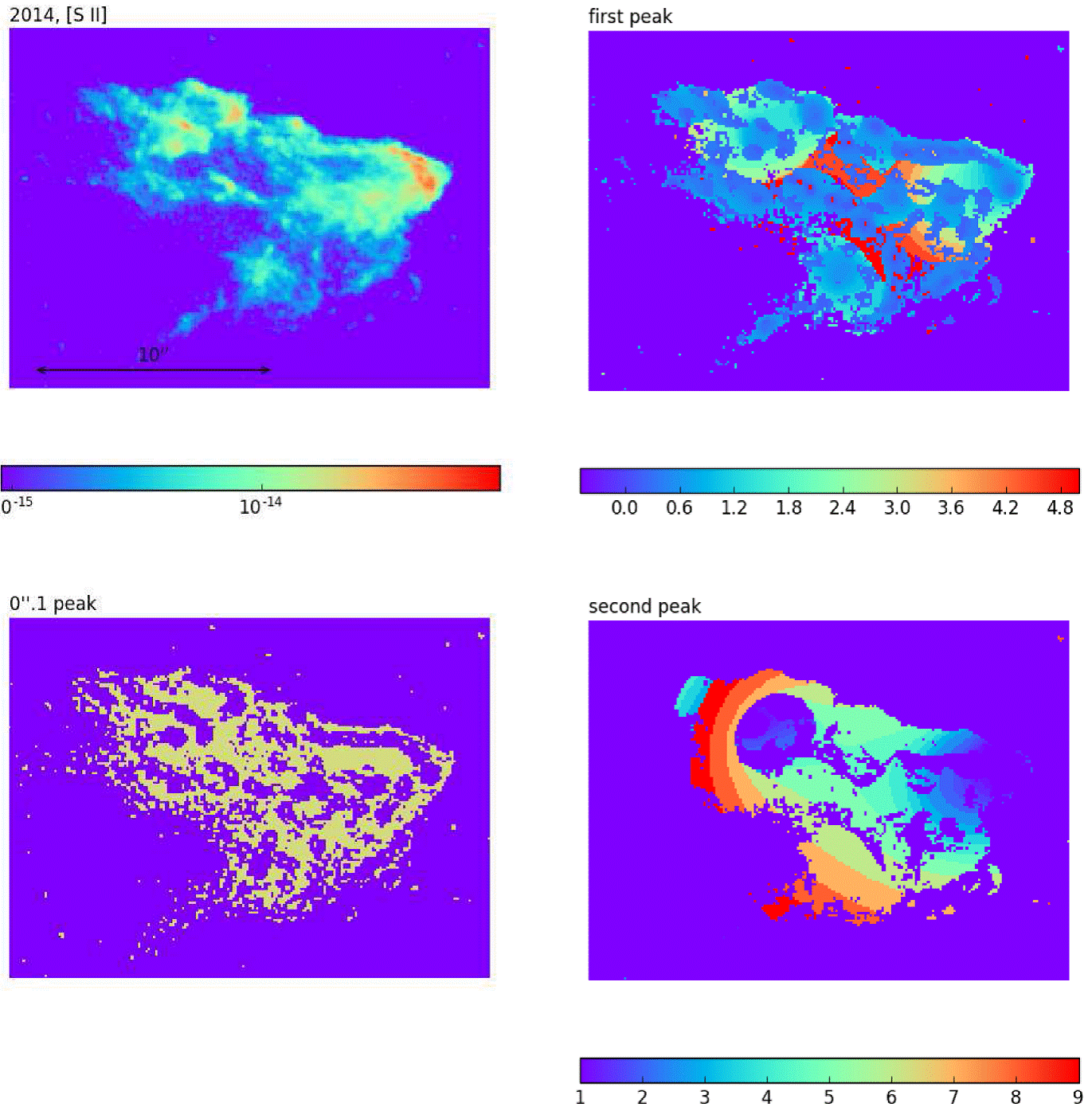
Fig. 2 Top left frame: the 2014 [S II] structure of HH 1 (shown with the logarithmic scale given in erg cm-2s-1 arcsec-2 by the bottom bar). Bottom left frame: the spatial distribution of the pixels that have a peak at the lowest (σ = 0´´.1) wavelet size. Top right: spatial distribution of the first σ > 0´´.1 peak of the wavelet spectra of the emitting pixels (the color scale shows the characteristic sizes, given in arcsec by the bottom bar, corresponding to the position of the first peak). Bottom right: the spatial distribution of the second peak in the wavelet spectra. The spectra of many of the emitting pixels do not show a second, σ > 0´´.1 peak. The color figure can be viewed online.

The spatial distributions of the first peak with σ > 0´´.1 (see Figures 2 and 3) show that characteristic sizes of ≈ 0´´.3 are found at the positions of theHH1and2knots,andthatsizesofupto≈5´´ are found in the more diffuse emitting areas of these objects. The second peak (with σ > 0´´.1) indicates characteristic sizes of ≈ 3´´ → 10´´, with the larger sizes (basically corresponding to the size of the full emitting regions of the HH objects) located in the periphery of the HH 1 and 2 emission regions (see Figures 2 and 3).
4. The characteristic size distribution functions of HH 1/2
4.1. General Description
Figures 4 and 5 show the characteristic size distributions of HH 1 and 2 (shown as the distribution σf (σ) as a function of log10 σ) obtained from the four observed epochs in [S II] and Hα. These size distributions have been computed in the way described in Appendix A. This Appendix also describes the general properties of the distributions.

Fig. 4 Characteristic size distributions derived for the [S II] emitting regions of HH 1 (left) and HH 2 (right). The distributions obtained from the 1994 (top), 1997, 2007 and 2014 images (bottom) are shown.

Fig. 5 Characteristic size distributions derived for the Hα emitting regions of HH 1 (left) and HH 2 (right). The distributions obtained from the 1994 (top), 1997, 2007 and 2014 images (bottom) are shown.
In contrast to the wavelet spectra of individual pixels of HH 1 and 2, which have at most three peaks as a function of σ (see § 3), the distributions of the characteristic sizes (obtained from all of the individual pixels) have 5-6 peaks. All size distributions have a peak at the smallest, σ = 0´´.1 wavelet size. As discussed in § 3 and Appendix A, these peaks appear to be associated with the negative rings around the brighter knots, and we will not discuss them further.
The main, striking, characteristic of the size distributions is that they have a series of relatively well defined peaks, with similar separations in log10 σ, corresponding to factors of ≈ 2 → 3 in the characteristic sizes of the successive peaks. The peaks indicating lower characteristic sizes have σ ≈ 0´´.3 → 0´´.5 (see Figures 4 and 5). Since these sizes correspond to the characteristic radii of the emitting structures, it is clear that they are well resolved at the 0´´.1 resolution of the HST images.
The peaks indicating the largest characteristic sizes (see Figures 4 and 5) lie in the 4´´→ 9´´ range.
These sizes are similar to the size of the full emitting regions of HH 1 and 2.
When comparing the spectra obtained for the successive time frames, one sees that there are small shifts (mainly to larger characteristic sizes) of the local maxima. This effect is discussed in more detail in the two following subsections.
4.2. [S II] characteristic sizes
Some of the features seen in the [S II] HH 1 size distributions (see Figure 4) are:
a peak at σ = 0´´.4 (indicated with the dashed, vertical line labeled as1) which shows up in the 1997 (and possibly also in the 1994) frame, but is absent in the 2007 and 2014 frames,
a peak at σ = 0´´.7 (vertical line labeled bs1), visible in the size distributions of all frames,
a peak at σ = 1´´.2 (vertical line labeled cs1), which is shifted to a somewhat larger, σ ≈ 1′′.4 size in the 2007 and 2014 frames,
a “large size peak” at σ = 4´´ (vertical line labeled ds1 ) which becomes progressively shifted (with time) to larger sizes, up to σ ≈ 5´´ in the 2014 frame.
The [S II] HH 2 size distributions have:
a broad structure centered around σ = 0´´.5 (labeled as2), which is seen as a single peak only in the 2007 frame,
a peak at σ = 1´´.4 (labeled bs2), which is not present in the 2014 frame,
a peak at σ = 3´´ (labeled cs2), which becomes a strong feature in the 2014 frame,
a “large size peak” at σ ≈ 6´´.5 (labeled ds2, which is not seen as a peak in the 1994 frame, and migrates to larger sizes from 1997 to 2014.
4.3. Hα Characteristic Sizes
Some of the features seen in the Hα HH 1 size distributions (see Figure 4) are:
a peak at σ = 0´´.3 (labeled ah1) which shows up in the 2007 and 2014 frames, but is absent in the 1994 and 1997 frames,
a peak at σ = 0´´.7 (labeled bh1),
a peak at σ = 1´´.2 (labeled ch1), which apparently migrates to a somewhat smaller, σ = 1´´ size in the 2014 frame,
a peak at σ ≈ 1´´.8 (labeled c′h1), which migrates to somewhat larger sizes with increasing time, and becomes a dominant feature of the distribution in the 2014 frame,
a “large size peak” at σ ≈ 6´´ (labeled dh1). The Hα HH 2 size distributions have:
a peak at σ = 0´´.4 (labeled ah2) only appearing in the 2014 frame,
a peak at σ = 0´´.8 (labeled bh2), progressively migrating to somewhat larger sizes with time,
a peak at σ = 1´´.5 (labeled ch2),
a “large size peak” at σ ≈ 8´´(labeled dh2, also migrating to larger sizes.
5. 2D characteristic size distributions
It is also possible to carry out a characterization of the emission structure of HH 1 and 2 using 2D, anisotropic wavelets. This is interesting because it is to be expected that an outflow may have different structures along and across the outflow axis.
We choose an elliptical “Mexican hat” wavelet kernel of the form:
where σx and σy are the half-widths of the central peak along and across the outflow axis, respectively. A similar 2D version of the “Mexican hat” wavelet has been used by Riera et al. (2003) to study the characteristics of the HH 110 outflow.
We then convolve the 2014 Hα images of HH 1 and 2 with 2D wavelets with σx
and σy from 1 to 61 pixels (0´´.1 to 6´´.1). In the resulting
four-dimensional spectrum (with axes x, y, σx and σy), for all
the spatial pixels (x,y) with Hα intensities larger Ic = 1.5 × 10⁻¹⁵ erg
s-1 cm-2 arcsec-2 we compute the wavelet
spectrum Sx,y(σx,σy). For all these pixels we find
the positions (σx,σy)m of the two peaks with smaller
In Figure 6, we show the resulting 2D characteristic size distributions σxσyf2D(σx,σy) (corresponding to the σf(σ) 1D distributions shown in Figures 4 and 5) obtained from the 2014 Hα maps of HH 1 and 2. Because of the relatively small number of emitting pixels within HH 1 and 2, these distributions are quite noisy. However, it is clear that a wide range of (σx,σy) combinations are present in different regions of HH 1 and 2, implying structures with sizeable elongations both along and across the outflow axis.

Fig. 6 2D characteristic size distributions of the 2014 Hα maps of HH 1 (top) and HH 2 (bottom). The axes of the two frames are the characteristic sizes σx (along) and σy (across the outflow axis), given in arcsec. The normalized distribution functions σx σy f2D (σx , σy ) are shown with the logarithmic color scale given by the top bar. The color figure can be viewed online.
This calculation of f2D (σx , σy) characteristic size distributions is only meant as an illustration of the characteristsics of a 2D analysis. A full analysis of this kind should include an application of arbitrary rotations φ to the image, after which the convolution with the elliptical wavelet g (see equation 1) should be made. We have not carried out such a study.
6. Conclusions
We have computed the wavelet spectra of 4 epochs of Hα and [S II] HST images of HH 1 and 2. The spectrum of each pixel (corresponding to the intensity as a function of radius σ of the wavelets) shows one, two or three maxima. The values of σ at which these maxima are found correspond to the characteristic sizes of emitting structures in the region around each pixel.
We first show maps of the characteristic sizes found for the [S II] emission of HH 1 and 2, observed in 2014 (see Figures 2 and 3). These maps show that the brighter knots of HH 1 and 2 are angularly resolved structures, with characteristic radii of ≈ 2−3´´. The fainter regions of these objects have characteristic sizes ranging from 3´´ up to ≈ 10´´ (i.e., similar to the full size of the HH 1 and 2 emission regions).
We then compute the distributions of the characteristic sizes found from the wavelet spectra of all of the emitting pixels in the HH 1 and HH 2 regions. These distributions show a number of peaks as a function of wavelet radius σ (Figures 4 and 5 showing the distributions obtained for the four epochs of [S II] and Hα images, respectively). The distributions plotted as a function of log10 σ show a number of peaks, with spacings corresponding to factors of ≈ 2 − 3 in the positions of the successive maxima. This result indicates that HH 1 and 2 have a hierarchy of structures with logarithmically spaced angular radii in the 0´´.3 → 10´´ range.
These peaks in the size distributions with spacings of factors ≈ 2 → 3 (see Figures 4 and 5) are a dominant feature of the knot size distributions of HH 1 and 2. However, their origin is unclear. The observed spacings between characteristic sizes could be:
the result of an instability in the flow with a discrete set of dominating modes,
the reflection of an ejection time-variability (from the outflow source) of appropriate characteristics,
structures produced by a hierarchy of knot merging processes.
In all of these scenarios, line of sight superpositions of emitting structures will also have an important effect on the observed characteristic size spectra.
We find that the [S II] and Hα emissions (of both HH 1 and 2) have somewhat different size distributions (this can be seen comparing the corresponding columns of Figures 4 and 5). Different size distributions might be expected in structures formed by curved shocks, which have different [S II]/Hα line ratios depending on the local normal shock velocity (as can be seen from predictions for plane-parallel, steady shocks such as the ones of Hartigan et al. 1987).
A comparison between the size distributions of the four indicates show that the relative height of the peaks changes with time, and that the positions of the peaks show small displacements. These displacements occur mostly towards larger characteristic radii of the emission structures.
This result clearly argues against the straightforward expectation of a turbulent cascade, in which large structures (eddies) break up into smaller scale structures. The expansion that we see at all scales could correspond to a general expansion of the HH objects, or to merging processes of the emitting knots.
Merging of smaller structures to form larger scale structures is predicted from solutions of Burgers’s equation (see Tatsumi & Kida 1972; Tatsumi & Tokunaga 1974; Raga 1992). As the solutions of Burgers’s equation have strong resemblances to hypersonic flows, it is possible that we are seeing such an effect in HH 1 and 2. These HH objects have also been modeled numerically by Hansen et al. (2017) as a system of interacting clumps. This sort of “inverse cascade” would be an indication that we are not able to resolve the (forward) turbulent cascade at scales below the injection produced by the jet.
Even though we detect rather marginal displacements in the peaks of the size distribution functions (see § 4.2 and 4.3), it is evident that the shifts in the logarithms of the values of the peak positions are approximately scale independent. For example, for peak ds1 (located at σ ≈ 4´´, see Figure 4) we see a ∆σ20 ≈ 1´´ over the 20 year time span of the HST images. This corresponds to a yearly expansion rate of ∆σ1/σ ≈ 0.01 yr-1. Similar values of ∆σ/σ are found for all of the peaks with detected shifts. For the larger scales of HH 1/2 (of ≈ 10´´) these expansion rates correspond to a ≈ 200 km s-1 velocity (similar to the dispersion of the proper motions of the HH 1/2 condensations, see Raga et al. 2016a, b), and for the smaller scales (of ≈ 3´´) the expansion velocity is ≈ 60 km s−1 (assuming a distance of 400 pc to HH 1/2). These two velocities are highly supersonic at the temperature of ≈ 104 K of the emitting regions of HH 1/2 (see Raga et al. 2016c).
If one assumes that the expansion that we observe at all scales is time-independent, one obtains a τ = σ/∆σ1 ≈ 100 yr estimate for the time at which HH 1 and HH 2 had vanishing sizes. From this argument, one can conjecture that HH 1 and 2 were formed ≈ 100 yr ago, at positions ≈ 15´´ closer the outflow source than the present positions of these two objects (for a proper motion of ≈ 300 km s-1 for HH 1 and 2). This formation of HH 1 and 2 at large distances from the outflow source can easily be interpreted in terms of internal working surfaces formed by a variable velocity jet (see, e.g., Raga et al. 2015c and references therein).
Our present work is an effort to obtain a quantitative description of the time-evolution of the emission structures of HH 1 and 2. Though this can be done in different ways, we have focussed on obtaining wavelet spectra, and studying the size distributions that can be obtained from such an analysis. It will be interesting to apply this analysis to the structures of other HH objects, as well as to synthetic emission maps calculated from gasdynamical or MHD simulations of HH jets.