


 nueva página del texto (beta)
 Inglés (pdf)
 Artículo en XML
 Referencias del artículo
 Enviar artículo por email
 Citado por SciELO
  Similares en
SciELO
Similares en
SciELO 
 Permalink
1. Introduction
Hot molecular cores (HMCs) are considered to be the birthplace of high-mass stars (e.g., Kurtz et al. 2000; Garay & Lizano 1999). Thus, to study their physical properties, dynamics, and evolution is crucial for advancing our understanding of high-mass star formation. HMCs are detected mainly by emission of high-excitation molecular lines (e.g., CH3CN and NH3) and by millimeter continuum emission from warm dust. A detailed overview of star formation was presented by Stahler & Palla (2005), while a review of high-mass star formation was published by Zinnecker & Yorke (2007).
Water maser emission is a common phenomenon in the neighborhood of newly-formed high-mass stars (e.g., Codella et al. 2004; Trinidad et al. 2003; Hofner & Churchwell 1996). However, the relationship of the H2O masers to the star formation environment is still not fully understood. It is accepted that their presence implies the existence of at least one embedded YSO (e.g., Garay & Lizano 1999). For ultra compact H II regions (UC H II) with cometary morphologies, Hofner & Churchwell (1996) showed that the water masers were almost always located in clusters, near, yet offset, from the cometary arc; and for other morphologies the masers were often projected onto the ionized gas. Hofner & Churchwell (1996) also found that water masers were related to hot NH3 clumps (and YSOs) rather than to the ionized gas of the H II regions. The latter was also observed by Cesaroni et al. (1994) in a sample of 4 molecular cores.
G12.21-0.10 (G12 hereafter), located at a distance of 13.5 kpc (Churchwell et al. 1990), has been classified as a cometary UC H II region with extended emission (de la Fuente et al. 2009a; de la Fuente 2007; Kim & Koo 2001). C17O observations finding a molecular clump coincident with the UC emission were reported by Hofner et al. (2000). This region also presents emission of hot and dense chemically enriched gas tracers (see Table 1), and has been also observed in infrared (IR) surveys (de la Fuente et al. 2009b; de la Fuente 2007; De Buizer et al. 2003). Hence, it was deemed a prime candidate for a HMC by De Buizer et al. (2003).
Table 1 Previous molecular observations toward G12
| Molecule | Tk (K) | n(H2) (cm−3 ) | Size (arcsec) | N(H2) (cm−2 ) | Ref.a |
|---|---|---|---|---|---|
| NH3 | · · · | 4.8×10⁵ | 4.0 | 5.2×10²³ | 1 |
| CS | · · · | 8.1×10⁵ | · · · | 2.0×10²³ | 2,5 |
| CH3 CN | 80-90 | 106 -109 | · · · | 2.0×1025 | 3,1 |
| CH3OH | 56800 −24 | 107 | 1.3 | 1.2×1025 | 4 |
a(1) Cesaroni et al. 1992; (2) Plume et al. 1997; (3) Olmi et al. 1993; (4) Hatchell et al. 1998, (5) Shirley et al. 2003.
In G12, H2O and CH3OH maser emission is observed toward the molecular clump, not towards the ionized gas (Kurtz et al. 2004). In particular, the water masers are offset by ≈4′′ (or 0.26 pc at 13.5 kpc) from the UC H II region, suggesting the location of a deeply embedded, young high-mass star (Hofner & Churchwell 1996). In addition, Kurtz et al. (2004) found that a strong water maser feature in this cluster coincides spatially with both Class I (44 GHz) and Class II (6.67 GHz) CH3OH masers. Thus, G12 is an interesting candidate for studying the nature and formation of water and methanol masers and for understanding their relation to molecular gas and high-mass star formation.
In § 2 we describe the radio continuum and spectral line observations and data reduction. In § 3 we present the observational results and analysis as follows: 1. We show that the 13CS (1−0 and 2−1) transitions trace the hot and optically thin dust clump in G12; 2. We calculate the physical characteristics of this clump using NH3 data to confirm that it is a hot molecular core. In § 4 we discuss the 13CS and NH3 data in the context of the HMC interpretation. A summary is presented in § 5.
2. Observations and data reduction
2.1. Owens Valley Radio Observatory (OVRO) Observations
The 13CS(2−1) and H41α line observations were made with OVRO during March and April 1996. The equatorial and high resolution configurations were used, providing baselines from 30 to 240 m. Cryogenically cooled SIS receivers provided typical SSB system temperatures of 220-350 K. The digital correlator was split into two bands to observe the 13CS(2−1) (ν0 = 92.49430 GHz) and H41α (ν0 = 92.03445 GHz) lines with 30 MHz (≈100 km s−1) and 60 MHz (≈200 km s−1) bandwidths, and 62 and 60 Hanning-smoothed channels, respectively. This configuration gives a spectral resolution of 0.5 MHz (1.6 km s−1) for the 13CS(2−1) line and 1 MHz (3.3 km s−1) for the H41α line.
In addition, simultaneous continuum observations at 3 mm were made using a 1 GHz bandwidth analog correlator. The quasars NRAO 530, 3C 454.3, B1908−202, and B1749+096 were observed to track amplitude and phase variations. The bandpass calibration and flux scale were established by observing 3C 273. The absolute flux uncertainty was estimated to be ≈20 %, and the initial calibration was carried out using the Caltech MMA data reduction package (Scoville et al. 1993). Further data reduction and mapping were done with the AIPS software package. The continuum obtained from the line-free channels was subtracted from the 13CS and H41α emission lines in the (u,v) plane using the program UVLIN in AIPS. Finally, Gaussian fits to the observed spectra were made with the CLASS software package.
2.2.1. Radio-Continuum Emission
High angular resolution continuum observations at 0.7, 2, and 3.6 cm toward G12 were made with the VLA8 in its CnB configuration on 1996 January 29. Two 50 MHz bands were observed, each one including both right and left circular polarizations. We used a subarray of 12 antennas for 7 mm observations and the remaining 15 antennas were employed for 2 and 3.6 cm observations. The flux and phase calibrators were 3C286 (1.45, 3.40 and 5.23 Jy at 0.7, 2, and 3.6 cm) and B1923+210 (1.0, 1.8 and 1.0 Jy; flux densities meassured at 0.7, 2, and 3.6 cm respectively).
In addition, low angular resolution VLA observations at 3.6 cm in the D configuration toward G12 were made on 2005 April 03. As before, two 50 MHz bands were observed, each one including both right and left circular polarizations. The flux and phase calibrators were 3C 286 (5.23 Jy) and J1832−105 (1.28 Jy), respectively.
The calibration and imaging for both high and low angular resolution observations were made following standard procedures in AIPS. Self-calibration in phase only, and Multi-Resolution Cleaning were performed for the low angular resolution data.
2.2.2. NH3 and 13 CS(1−0) Emission
Observations of NH3 were made with the VLA in its DnC configuration on 2004 June 06. Both transitions (2,2) and (4,4), with rest frequencies of 23722.631 and 24139.417 MHz, respectively, were observed. In order to include the main line and one pair of hyperfine satellites, the spectral line correlator was split into two overlapping bands of 64 channels each, centered at 2.30 and 0.76 MHz higher and lower than the expected line frequency for (2,2) and 1.06 and 1.24 MHz for (4,4). The Doppler tracking center velocity was set to 24 km s−1 (VLSR) and the total velocity coverage was 94 km s−1, obtaining a frequency resolution of 97.656 kHz (1.25 km s−1). The flux, phase and bandpass calibrators were 3C 286 (2.6 Jy), J1820−254 (0.53 Jy) and J1924−292 (9.1 Jy), respectively. Calibration and data reduction were done following standard line procedures of the AIPS software package. All images were obtained using the task IMAGR with ROBUST = 0, while the spectra were obtained with task ISPEC after combining the two overlapping bands into a single 71 channel cube; the cube moment maps were made using the task XMOM. Gaussian fits to the observed spectra were made using the CLASS software package.
During the same run, 13CS(1−0) observations at the rest frequency of 46.24757 GHz, were also carried out. A central bandpass velocity of 24 km s−1 was used. Flux, phase and bandpass calibrators were the same as for NH3, as well as the calibration and data reduction. A natural weighting was used to generate the images.
3. Observational results and analysis
3.1. Radio Continuum Emission
The 21 cm NVSS contour map (Condon et al. 1998) superposed on the 3.6 cm low angular resolution VLA-D map in gray-scale toward G12 is shown in Figure 1a Left. The morphologies of both emissions match at different scales in this region, and are in agreement with 21 cm observations from Kim & Koo (2001, their Figure 1 g). Six continuum peaks are detected at 3.6 cm, one of which corresponds to the UC source.
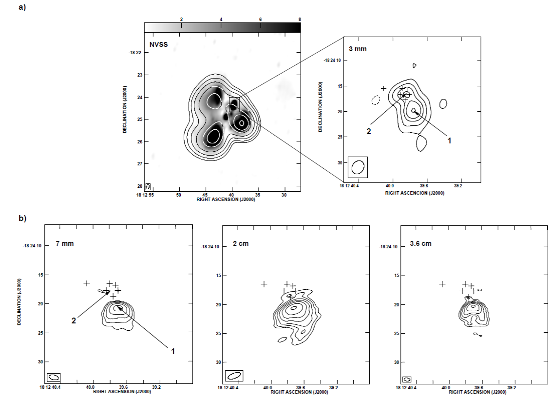
Fig. 1 G12.21-0.10 (G12). a) Left: 21 cm NVSS map (contours) superposed on the 3.6 cm VLA D-configuration image in gray-scale (de la Fuente 2007).
The 3 mm continuum emission toward the UC source is split into two peaks (see Figure 1a Right). They are separated by ≈4´´ (0.26 pc at a distance of 13.5 kpc); one of them corresponds to the UC H II region (labeled as 1), while the other (labeled as 2) coincides with a water maser group reported by Hofner & Churchwell (1996). Due to the possible relation between these masers and the molecular clump reported by Hatchell et al. (2000), we will refer to Peak-2 as the molecular clump. The peak positions of the 3 mm continuum emission from the UC H II region and the molecular clump are reported in Table 2.
Table 2 Detection summary
| Observation | Wavelength (cm) | Right Ascencion (J2000) | Declination (J2000) | Source |
|---|---|---|---|---|
| VLA continuum | 0.7, 2, & 3.6 | 18h 12m 39.8s | -18◦ 24′ 21′′ | UC H II region |
| OVRO H41α | 0.33 | 18h 12m 39.6s | -18◦ 24′ 21′′ | UC H II region |
| OVRO continuum | 0.30 | 18h 12m 39.8s | -18◦ 24′ 21′′ | UC H II region (Peak-1) |
| OVRO continuum | 0.30 | 18h 12m 39.8s | -18◦ 24′ 17′′ | molecular clump (Peak-2) |
| OVRO 13CS(2−1) | 0.32 | 18h 12m 39.7s | -18◦ 24′ 18′′ | molecular clump |
| VLA NH3(2-2) | 1.26 | 18h 12m 39.8s | -18◦ 24′ 18′′ | molecular clump |
| VLA NH3(4-4) | 1.24 | 18h 12m 39.8s | -18◦ 24′ 18′′ | molecular clump |
| VLA 13CS(1−0) | 0.65 | 18h 12m 39.8s | -18◦ 24′ 18′′ | molecular clump |
| VLA continuuma | 1.3 | 18h 12m 39.7s | -18◦ 24′ 21′′ | UC H II region |
aThis is the continuum obtained from NH3 observations.
High angular resolution continuum observations at 0.7, 2, and 3.6 cm are displayed in Figure 1b. They show that the radio continuum emission is only associated with the UC H II region. Then, the observed emission at 3 mm and the lack of emission at 0.7, 2 and 3.6 cm toward the 3 mm peak-2, suggest that the 3 mm continuum emission toward the molecular clump could arise from dust rather than ionized gas. Integrated continuum flux densities of the ionized gas, rms noise, beam, and deconvolved sizes for these wavelengths are given in Table 3.
Table 3 Continuum parameters
| Region | Telescope | λ (cm) | Sv (mJy)a | Beam Size; P.A (arcsec; deg) | RMS Noise (mJy beam−1) | Deconvolved Size (arcsec) |
|---|---|---|---|---|---|---|
| UC H II | VLA CnB | 3.6 | 220 | 2.31 × 0.91; −70 | 0.31 | 5 × 4 |
| VLA CnB | 2.0 | 200 | 1.04 × 0.55; +80 | 0.21 | 8 × 7 | |
| VLA CnB | 0.7 | 160 | 1.65 × 0.83; +77 | 0.58 | 4 × 5 | |
| Molecular clump | OVRO | 0.3 | 150 | 2.82 × 2.32; −43 | 1.70 | 3 × 1 |
| Extended emission | VLA D | 3.6 | 1320 | 12.50 × 7.30; −13 | 0.15 | 210 × 156 |
aUncertainties in the integrated flux densities are estimated to be about 5% at 3.6, 10% at 2 cm, and 20% at 7 mm. The deconvolved sizes and uncertainties in flux densities were obtained using the task IMFIT in AIPS.
3.2.1. H41α
The H41α (≈3.3 mm) emission is only detected toward the UC H II region; no emission is detected toward the molecular clump. The H41α emission has a similar distribution as the radio continuum observed at 7 mm shown in Figure 1b.
The H41α spectrum toward G12 is shown in Figure 2 (upper panel). Line emission was detected in the velocity range of ≈10 to 45 km s−1, with a peak at about 30 km s−1. The results of the Gaussian fit of this recombination line are presented in Table 4.
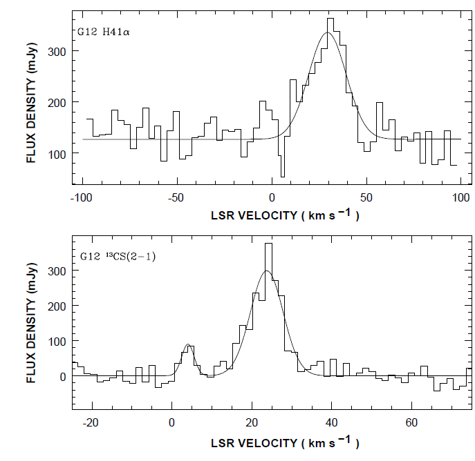
Fig. 2 H41α and 13CS(2−1) spectral lines. The solid line represents the best adjusted Gaussian in each spectrum. The CS spectrum also shows an unexpected weaker line at ≈4.5 km s−1. A possible candidate for this line is C3S.
Table 4 13CS(2−1) and H41α results
| Linea | Beam Size; P.A. (arcsec; deg) | RMS noise (mJy beam−1) | Sv b (mJy) | VLSR km s−1 | ΔVobs km s−1 | Deconvolved Sizec (arcsec) |
|---|---|---|---|---|---|---|
| 13CS(2-1) | 3.18 × 2.51; −43 | 35 | 300 | 23.7±0.1 | 9.4±0.5 | 4.5 × 2.0 |
| H41α | 3.18 × 2.51; −43 | 35 | 335 | 29.4±1.2 | 23.9±3.1 | · · · |
aThe spectral resolution of the CS line is 1.6 km s−1 and that of the H41 line is 3.3 km s−1.
bFrom peak channel at 23 km s−1 for 13CS(2−1), and at 30 km s−1 for H41.
cThe size of the source was obtained from the moment 0 image using IMFIT in AIPS.
The H41α velocity, 20−25 km s−1is similar to that of the molecular emission from 13CO(1−0), C34S(2−1), and C34S(3−2) both from Kim & Koo (2003) and this work (see below). In addition, the H41α LSR central velocity is in agreement with that reported by Kim & Koo (2001) using H76α for three positions in the extended emission (≈27 km s−1 on average, see their Figure 1g). The ionized gas in G12, present at different scales (UC and extended emission; see Figure 1), coexists with the molecular gas and originates in the same star forming region.
3.2.2. 13 CS(2−1)
Figure 3 shows the channel maps of the 13CS(2−1) line emission superposed on the 3.6 cm continuum emission. The deconvolved size of this molecular region is ≈ 4.′′5 × 2′.′0 (0.36 × 0.16 pc) with the major axis oriented approximately in the E−W direction, while the 13CS(2−1) peak emission observed at VLSR = 24 km s−1 is blueshifted (≈5 km s−1) with respect to the H41α. The 13CS(2−1) line spectrum is shown in Figure 2 (lower panel). Observed parameters (flux densities, rms noise, beam, and deconvolved sizes) for 13CS(2−1) toward G12 are presented in Table 4.
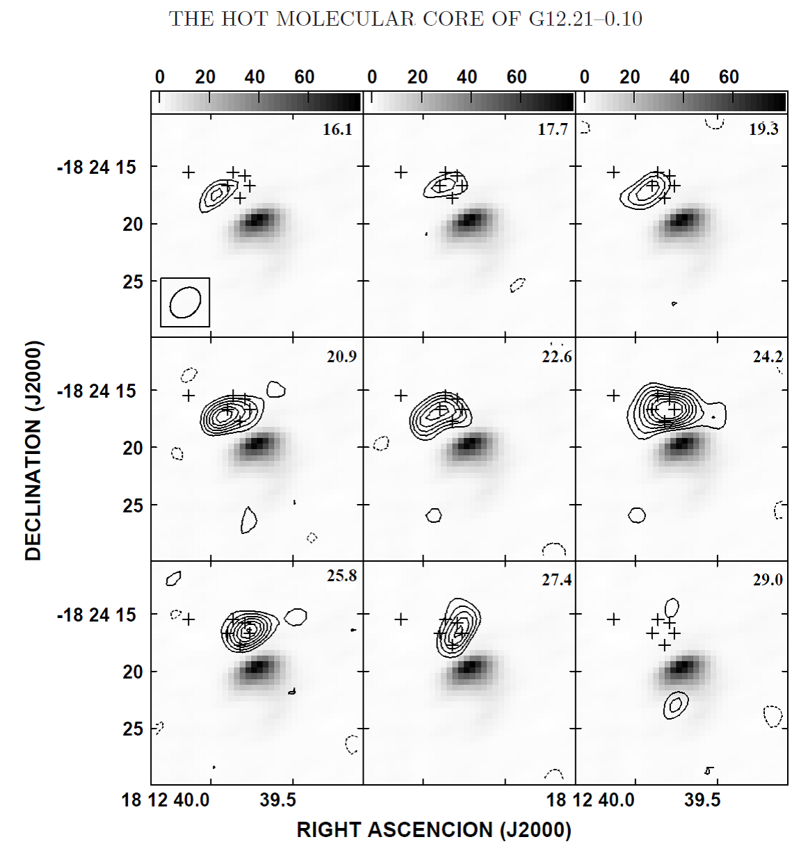
Fig. 3 13CS(2−1) channel maps (contours) with channel width of 1.62 km s−1 are shown between 16 and 29.0 km s−1 superposed on the radio continuum emission at 3.6 cm (VLA-CnB, gray-scale) of G12.
Comparing the 13CS(2−1) line and the 3.6 cm (VLA-CnB) continuum emission, we note that the 13CS(2−1) emission is not spatially associated with the UC region in G12, but rather with the molecular clump and the group of water masers. This result suggests the presence of a molecular clump spatially associated with the 3 mm continuum emission (Peak-2), not far from the UC H II region (see Table 2).
Figure 2 (lower panel), shows that in addition to the 13 CS(2−1) line at VLSR = 24 km s−1 , a weaker component at 92.49284 GHz is marginally detected at VLSR = 4.5±0.5 km s−1 assuming the 13CS(2−1) rest frequency; and ∆V = 3.6±1.1 km s−1. A possible candidate to explain this weak emission is the molecule C3S (ν0 = 92.48849 GHz; Morata et al. 2003) at VLSR = 14.1±0.5 km s−1. Although this molecular line seems to be real, given the low signal- to-noise (≈2.5σ at the peak), we cannot determine the physical parameters of the molecular gas from which this emission arises.
3.2.3. 13 CS(1−0)
Figure 4 shows the channel maps of the 13CS(1−0) emission towards G12 superposed on the 13 CS(2−1) integrated map as comparison. Although 13 CS(1−0) and 13 CS(2−1) present different morphologies, both are spatially associated with the molecular clump (3 mm Peak-2). This morphological difference could in part be due to the different spatial resolution achieved for each molecular line. However, the 13CS(1−0) emission presents a complex morphology as revealed by each channel map (see also the integrated emission shown in the inset of the 27.2 km s−1 panel). This morphology shows a central double-component roughly in the East-West direction (labeled as E and W in the inset) with peak line emission observed at VLSR = 20 km s−1 and 23 km s−1, respectively. Another weak emission peak to the North (labeled as N) is also observed at VLSR = 26 km s−1.

3.2.4. NH 3
The NH3 emission is only detected toward the molecular clump (3 mm peak-2). The integrated NH3 spectra of the (2,2) and (4,4) transitions are shown in Figure 5. In the (2,2) transition the satellite lines are marginally resolved, and in (4,4) the satellite lines are blended into a single component.
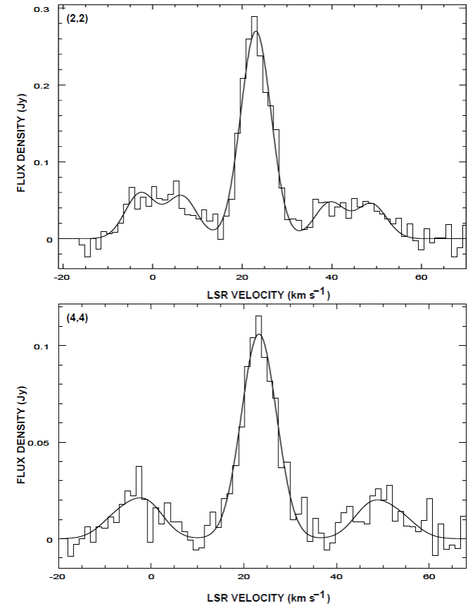
Fig. 5 NH3 integrated spectra of (2,2) and (4,4) transitions in the G12-HMC . The solid lines show Gaussian fits.
The two electric hyperfine components were fit with two Gaussians and the results of the fits are given in Table 5.
Table 5 NH3 line parameters
| Transition (J,K; line) | Beam Size; P.A. (arcsec; deg) | RMS Noisea (mJy beam−1) | Peak SV (mJy) | VLSR (km s−1) | ΔVobs (km s−1) | Deconvolved Size (arcsec) |
|---|---|---|---|---|---|---|
| (2,2; main) | 3.54×1.36; +60 | 4.4 | 260±5 | 23.1±0.3a | 8.1±0.7 | 3.8 × 3.0 |
| (2,2; inner satellites) | 3.54×1.36; +60 | 5.7 | 59±2 | 6.5, 39.7b | 9.5c | · · · |
| (2,2; outer satellites) | 3.54×1.36; +60 | 6.1 | 59±2 | -2.7, 48.9b | 8.5c | · · · |
| (4,4; main) | 4.29×1.18; +56 | 3.2 | 106±5 | 23.3±0.3a | 8.9±0.7 | 3.0 × 1.0 |
| (4,4; inner satellites) | 4.29×1.18; +56 | 3.3 | 16.0±0.8 | -0.7, 27.3b | 13.2c | · · · |
| (4,4; outer satellites) | 4.29×1.18; +56 | 3.3 | 16.0±0.8 | -6.7, 53.3b | · · · | · · · |
aUncertainties are from Gaussian fits. The flux densities are from a box covering the HMC.
bThese two velocity values correspond to satellite lines without fitting.
cAverage values between the corresponding pair from the Gaussian fitting.
The (4,4) main peak line flux density is weaker than that measured in the (2,2) line. The observed widths of 8-9 km s−1 are evidence of highly supersonic turbulent motions in the molecular gas (Garay & Lizano 1999). The observed line parameters, flux densities, rms noise, beam, and deconvolved sizes for both transitions (2,2) and (4,4) are presented in Table 5. Within the uncertainties, the (2,2) and (4,4) VLSR and ∆Vobs are in mutual agreement. The measured LSR velocities of both transitions are slightly smaller (≈1 km s−1) than those reported by Churchwell et al. (1990) and Cesaroni et al. (1992) for (2,2) and (4,4) using the Effelsberg 100 m telescope, while the ∆Vobs for (2,2) and (4,4) are ≈1 km s−1 and ≈4 km s−1 greater, respectively. The line width difference indicates motion of the hotter compact (4,4) gas relative to the cooler extended (2,2) gas as discussed in Cesaroni et al. (1992).
Neither the (2,2) nor the (4,4) spectra show detectable anomalies in the satellite hyperfine components like those observed toward S106 in the NH3 (1,1) transition (Stutzki et al. 1982). Hence we can assume that the populations in the metastable levels are in LTE. To calculate physical parameters of the region based on the NH3 spectra, we also assume that true intrinsic widths, ∆Vt, are equal to the observed values, ∆Vobs .
Optical depths for the main lines, τmain, of 3.5±0.5 and 8.0±0.5 for (2,2) and (4,4) transitions, respectively, were calculated numerically (Ho & Townes 1983, equation 1). The total optical depth can be calculated as τtot = (1/b)τmain where b represents the normalized (to total intensity) relative intensities of the main line. Parameter b values of 0.8 and 0.93 for (2,2) and (4,4) respectively were assumed (Ho 1977), obtaining τ2,2 = 4.4±0.5 and τ4,4 = 8.6±0.5. In addition, excitation temperatures (Texc) of 78±5 K and 35±5 K for (2,2) and (4,4) were calculated in a standard way by solving the transfer equation (Ho 1977; Ho & Townes 1983). The column densities for (2,2) and (4,4) transitions in terms of τmain, Texc and ∆Vt were computed through the τtot definition given by Ungerechts et al. (1986) using the respective Einstein coefficient for spontaneous de-excitation: A± (2, 2) = 2.23 × 10⁻⁷ s−1 and A±(4,4)=2.82×10⁻⁷ s−1. Hence N(2, 2) = 2.6±1.0× 1016 cm−2 and N(4,4)=2.0±1.0×1016 cm−2.
The rotational temperature, T42 = 77±10 K, was computed in terms of the (2,2) and (4,4) peak flux densities and velocity widths (see Table 5) considering the same solid angle for both emissions. Using this rotational temperature, a rotation level diagram for para-NH3 (Walmsley & Ungerechts 1983; Poynter & Kakar 1975) considering collisional transitions between K-ladders and transitions which follow the parity transition rule, and doing the calculations in statistical equilibrium derived by Walmsley & Ungerechts (1983) with the numerical computations of Danby et al. (1988) in detailed balance, we obtained a value for the kinetic temperature of Tk = 86±12 K.
4. Discussion
4.1. The Hot Molecular Core
The kinetic temperature (86 K), volumetric density (1.5×106 cm−3) and linear size (≈0.22 pc, assuming a distance of 13.5 kpc) generally coincide with the operational definition of HMC: hot (>∼ 100 K), dense (≈105 to 108 cm−3), and small (size <∼ 0.1 pc) molecular gas structures (Cesaroni et al. 1992; Garay & Lizano 1999). So, based on these characteristics, we suggest that the molecular gas clump detected in G12 is a hot molecular core (G12-HMC hereafter).
Several maps of the molecular line emission from the G12-HMC region are presented in Figure 6. No radio continuum source was detected toward the G12-HMC position (Figure 6a) where the group of H2O masers is located. This could be explained following the suggestion of Walsh et al. (2003) that 6.67 GHz CH3OH masers appear before an H II region is created. However, higher sensitivity observations are needed, since Rosero et al. (2016) have a 100% detection rate in the radio continuum toward 25 HMCs, when observed with much higher sensitivity of ≈3-10 μJy beam−1 rms.
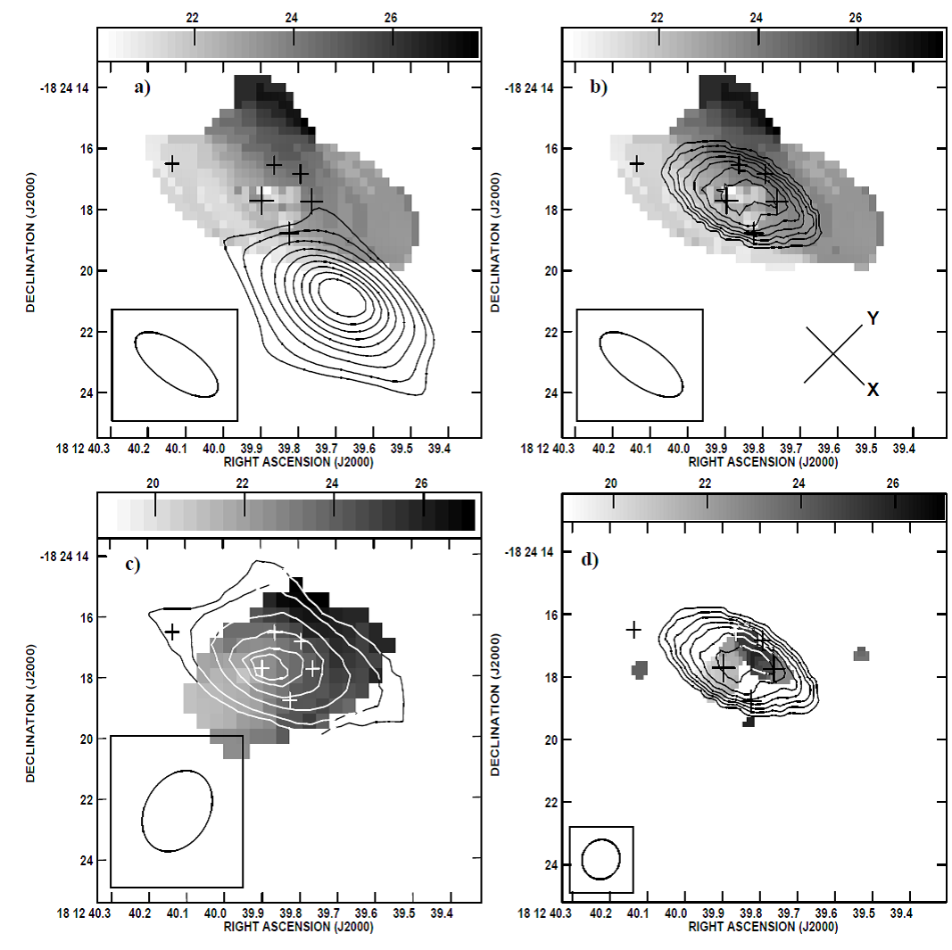
Fig. 6 G12-HMC. a) NH3(2,2) moment-1 map (gray-scale), superposed on the radio continuum emission at 1.3 cm (contours; UC H II region) obtained from line-free channels of the NH3(2,2) observations. Gray-scale is in the interval ≈ 19-27 km s−1.
The NH3 (2,2) and (4,4) emission clearly coincides with the molecular clump observed at 3 mm (see Figure 1a), as well as with the group of masers. The distribution of molecular gas from both transitions, NH3(2,2) and (4,4), is similar, although the NH3(4,4) emission is slightly more compact than the NH3(2,2) emission, suggesting that the hotter and denser gas is confined to a smaller-scale structure. Note that Figures 6c and 6d show the more extended and more compact emission, respectively.
The first moment map of the (2,2) transition shows a velocity gradient from E to N (following the nomenclature of the inset in Figure 4) from 21 to 28 km s−1 over ≈4′′ (≈30 km s−1 pc−1). A similar behavior is observed for the (4,4) moment-1 map (de la Fuente et al. 2010), but from 21 to 27 km s−1 over ≈3′′ corresponding to 25 km s−1 pc−1. For 13 CS(1−0), from ≈20 to ≈26 km s−1 , we obtain a velocity gradient of ≈3 km s−1 arcsec−1 (or 45 km s−1 pc−1), and for the 13CS(2−1) emission ≈28 km s−1 pc−1, which is similar to that of the NH3(2,2) map (compare the grey-scale bars in Figures 6a and 6c). The 13CS and NH3 emission coincide in position and kinematics, which suggests no chemical differentiation in the HMC.
In addition to the velocity gradient from E to N for 13CS(1−0), a velocity gradient from W to N of ≈1.5 km s−1 arcsec−1 (or 23 km s−1 pc−1) is also estimated. A comparison of these results with those reported for Orion-IRc2 HMCs (Chandler & Wood 1997) suggests that 13CS(1−0) is a good candidate line to trace the internal structure of HMCs as observed in Figure 6d.
Assuming that the 3 mm flux density is due to warm dust, we derive a clump mass Mclump = gSν d2 / κν Bν (Td) (e.g., Beltrán et al. 2006) for the G12-HMC of ≈ 2.0×10³ M⊙, where a gas-to-dust ratio of g = 100 and a dust mass opacity coefficient of κ112 = 0.2 cm2 g−1 (Ossenkopf & Henning 1994) were adopted. A flux density of 0.15 Jy (Table 3), a distance of 13.5 kpc, and a temperature Td = 86 K (Table 6) were assumed. In addition, considering a 3 mm deconvolved angular size of 1.7±0.5′′, and assuming that all hydrogen is in molecular form and that the clump is spherical, we determine a n(H2 )3mm ≈ 6.3×106 cm−3 , and thus a central hydrogen column density of N(H2) ≈ 4.2×1024 cm−2 (following e.g., Sánchez-Monge et al. 2017). Both values of n(H2 ) and N(H2 ) are in agreement with those reported in Table 1.
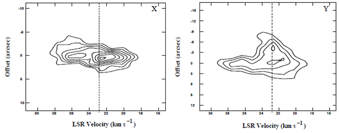
Fig. 7 NH3(2,2) position-velocity (PV) diagram of the HMC presented as grey-scale in Figure 6a and 6b. The plots are slices in the directions X and Y shown in the lower-right corner in Figure 6b.
The gas mass can be estimated from the 13CS(2−1) integrated line flux density assuming LTE, optically thin emission, and a fractional abundance for the 13CS molecule. Then, assuming the 12CS abundance is CS/H2 = 10−8, as estimated for the Orion Hot Core (van Dishoeck & Blake 1998), a 12CS/13CS ratio of 40 (Turner et al. 1973), and an excitation temperature ≃ 86 K from NH3 data, we obtain a gas mass of 6.3×10³ M⊙. Then, the mass ratio for G12-HMC is M(13 CS)/M(H2 ) ≈ 3. This discrepancy in the estimated mass can be explained in terms of the uncertainties in the adopted abundances, in the hot dust emission law, and in the gas to dust ratio.
Assuming a uniform density, a 13CS(2−1) virial mass of ≈2200 M⊙ is derived. This virial mass is in a better agreement with the NH3 virial mass (≈1500 M⊙ and ≈1800 M⊙) in comparison with that determined by Hatchell et al. (1998) via JCMT observations of CH3OH (1300 M⊙).
The volumetric density of H2 was also determined using equation 2 of Ho & Townes (1983). Considering the Einstein coefficient A(s−1) for the NH3(2,2) transition, the collision rate C(s−1) from Danby et al. (1988), we obtain n(H2 ) ≈ 1.5×106 cm−3 . The total NH3 column density was determined by summation of N(J,K) over all metastable rotational levels up to level J = 5, using Boltzmann’s Equation and assuming LTE. This density is somewhat less than that calculated using the 3 mm emission (≈6.3×106cm−3).
In addition, the H2 column density was calculated as N(H2)
= ΘS n(H2) where ΘS is the deconvolved linear
size in cm (3.′′4±0.1 ≈ 0.22±0.01 pc at 13.5 kpc; using
Since the virial mass estimations (2200 M⊙ from 13CS(2−1), and ≈1500 M⊙ to ≈1800 M⊙ from NH3) are about twice the ammonia gas mass (≈ 830 ±40 M⊙) we conclude that the G12-HMC may not be gravitationally bound. The physical parameters of this HMC are summarized in Table 6.
4.2. HMC Internal Heating Source
From the flux density at 3 mm and the upper limit at 7 mm from the molecular clump emission (3σ = 1.8 mJy), a spectral index of α>∼ 4.5 is obtained. This value suggests that the 3 mm emission arises from optically thin dust. If we consider that the dust in the molecular clump is only heated by external radiation, a lower limit to the dust temperature can be obtained using the formulation of Scoville & Kwan (1976, equation 9), under the assumption that no absorption exists between the ionizing star of the UC H II region and the clump. Using the 3 mm integrated flux density (see Table 3) and assuming an external O6.5 ZAMS ionizing star (Kim & Koo 2001, Lstar ≈ 1.5×10⁵ L⊙), a dust absorptivity κν ∝ ν+2, and a projected separation between the clump and the ionizing star (which is presumed to be at the focus of the cometary UC H II region) of 0.26 pc (4′′ at 13.5 kpc), we obtain Td = 130 K. This temperature is slightly greater than the values obtained with other molecular tracers (see Table 1, § 3.2.4 and § 4.2). However, not all luminosity of the O6.5 ZAMS ionizing star reaches the HMC. Considering a dilution factor of Ω/4π ≈0.06 (where Ω is the solid angle subtended by the ammonia core as seen from the ionizing star of the UC H II ), the fraction of incident luminosity from the UC H II on the HMC would be Linc ≈ 9000 L⊙. Using this quantity as the energy budget of the HMC, a dust temperature of about 70 K is estimated, which is similar to the kinetic temperature obtained in § 3.2.4 (86±12 K). This implies that an external heating source is not needed to explain the temperature of the core. However, the detection of water and methanol masers suggests the presence of a YSO in the HMC.
4.3. HMC Kinematics
There are different types of gas motion that can ocurr in HMCs, i.e., infall, rotation, and expansion/outflows. Outflows and rotation have been invoked to explain velocity gradients toward several HMCs (Cesaroni et al. 1998). In the case of rotation, flattened compact ‘disk-like’ structures with diameters greater than 0.1 pc (Garay & Lizano 1999, and references therein) are observed, and the velocity gradient may indicate the kind of rotation: differential or rigid body.
The NH3(2,2) position-velocity (PV) diagrams of G12-HMC are presented in Figure 7. We find no evidence of infall (e.g., redshifted absorption features). The central parts of the G12-HMC present larger velocity widths compared to the edges (≈6 versus 2 km s−1), and the overall structure of the HMC is elongated. The rotation scenario is possible.
The velocity widths across the HMC in the PV diagrams are also consistent with expansion motions. Two components on each side of the HMC central position(systemic velocity of ≈23 km s−1), have velocities of ≈26 km s−1 and ≈20 km s−1, suggesting that G12-HMC could be a structure with expansion motions at velocities of a few km s−1 in the SE-NW direction.
We have obtained images of integrated velocities from≈30to23kms−1 and from 23 to 18kms−1 using only the main line, and we do not see a clear spatial separation between this red-shifted and blue- shifted components. The opposite was found in the high-mass star forming regions G25.65+1.05 and G240.31+0.07, where high velocity molecular gas is associated with bipolar outflows (Shepherd & Churchwell 1996). Higher angular resolution observations are needed to confirm the rotation hypothesis and whether an outflow is present in the core.
5. Summary and conclusions
We present observations of radio continuum (0.3, 0.7, 2 and 3.6 cm) and spectral lines (H41α, 13 CS(2−1) and (1−0), NH3 (2,2) and (4,4)) toward the cometary H II region G12.21-0.10. Continuum emission is detected at all wavelengths toward the UC H II region. We also find 3 mm continuum emission toward a molecular clump located about 4′′ from the UC H II region. 13CS and NH3 emission is only detected toward the molecular clump and we do not find any chemical differentiation between these species.
We find evidence that the molecular clump is consistent with a hot (86 K), dense (1.5×106 cm−3), large (0.22 pc), and turbulent (∆Vobs ≈ 8 km s−1) molecular core. We also find that this hot molecular core shows a marginal velocity gradient in the SE- NW direction. Given that the HMC coincides with a water and methanol maser group, we speculate that a YSO, not detected in the centimeter radio continuum, could be forming inside the HMC.
Finally, we find that 13CS and NH3 are good candidates to trace the internal structure of HMCs. However, high angular resolution and higher sensitivity observations are needed to fully characterize this HMC.

