


 nova página do texto(beta)
 Inglês (pdf)
 Artigo em XML
 Referências do artigo
 Enviar este artigo por email
 Citado por SciELO
  Similares em
SciELO
Similares em
SciELO 
 Permalink
1. Introduction
Although KZ Hya (= HD 94033 = CD -24 9357) has been extensively studied and its nature wellestablished, the last thorough study of this star was that of Boonyarak et al. (2011). It is a well-known fact that this type of star needs continuous monitoring in order to deduce its nature correctly. In view of that, we present recent observations that, as will be seen, confirm the proposed behavior.
There has been some controversy with respect to the SX Phe, a high-amplitude Delta Scuti (HADS) star KZ Hya. Yang et al. (1985) suggested that there is a small amplitude light time effect and this was confirmed by Fu et al. (2008) with a much larger amplitude and longer period. Therefore, as has been said, it is understood that the light time effect with a short period and a small amplitude was occasionally covering the most changeable part of the light time effect of longer period and larger amplitude. Hence it can be seen that the observation time span should be long enough to confirm the light time effect. In a later study, the conclusions of Boonyarak et al. (2011) differed drastically from this interpretation. With one fundamental mode and its harmonics, they explained the observed light curves well without invoking the contribution of any companions. Hence, they confirmed that KZ Hya is a single-mode SX Phe star.
With a longer time span we expect to be able to dissipate any doubts on this matter.
2. Observations
Although some of the times of maximum light of this star have been reported elsewhere (Peña et al, 2015), we present new times of maxima and the detailed procedure followed to acquire the data. The observations were done at both the Observatorio Astronómico Nacional of San Pedro Mártir (SPM) and Tonantzintla (TNT), in México. Table 1 presents the log of observations as well as the new times of maximum light. Column 1 presents the date of the observation; Column 2 specifies the observer or group of observers. These correspond to the Advanced Observational Astronomy (AOA) course in 2015, and Escuela de Astronomía Observacional para Estudiantes de LatinoAmerica (ESAOBELA, LatinAmerican School of Observational Astronomy) in 2016 and 2017; the subsequent columns list the number of points, the time span in days and the number of maxima in each night; the time of maximum in HJD minus 2400000.0. The final columns list the technical details, telescope, filter and camera. The last column indicates in which observatory the data were acquired.
Table 1 Log of observing seasons and new times of maxima of KZ Hya
| Date yr/mo/day | Observers | Npoints | Time span (day) | Nmax | Tmax 2400000+ | Telescope | Filters | Camera | Observatory |
|---|---|---|---|---|---|---|---|---|---|
| 15/03/0607 | AOA15 | 155 | 0.16 | 1 | 57088.7971 | m1 | V | ST-1001 | TNT |
| 57088.8565 | |||||||||
| 15/03/0708 | AOA15 | 194 | 0.12 | 1 | 57089.7493 | m1 | V | ST-1001 | TNT |
| 15/03/3031 | DSP | 150 | 0.13 | 2 | 57112.7789 | m1 | V | ST-1001 | TNT |
| 57112.8385 | |||||||||
| 16/01/1112 | AAS, JG | 41 | 0.08 | 1 | 57399.9693 | 0.84 m | uvbyβ | SPM | |
| 16/01/2425 | ESAOBELA16 | 113 | 0.07 | 1 | 57412.8265 | m2 | V | ST-8300 | TNT |
| 16/03/1112 | PS, KL | 82 | 0.10 | 2 | 57459.8400 | m2 | V | ST-8300 | TNT |
| 57459.8989 | |||||||||
| 16/03/1213 | PS, KL | 52 | 0.06 | 1 | 57460.7921 | m2 | V | ST-8300 | TNT |
| 16/03/2223 | DSP | 154 | 0.13 | 2 | 57470.7894 | m1 | V | ST-8300 | TNT |
| 57470.8491 | |||||||||
| 16/03/2324 | DSP | 194 | 0.17 | 3 | 57471.7419 | m1 | V | ST-8300 | TNT |
| 57471.8013 | |||||||||
| 57471.8611 | |||||||||
| 17/01/1617 | ESAOBELA17 | 75 | 0.07 | 1 | 57770.9547 | m2 | G | ST-8300 | TNT |
| 17/01/1819 | ESAOBELA17 | 202 | 0.16 | 3 | 57772.8602 | m1 | V | ST-1001 | TNT |
| 57772.9198 | |||||||||
| 57772.9791 |
Notes: DSP, D.S. Piña; AAS, A.A. Soni; JG, J. Guillén; PS, P. Santillán; KL, K. Lozano; AOA15: S. Arellano, J. Diaz, X. Moreno, J. Ramírez, F. Ruíz, C. Téllez, K. Vargas, V. Vázquez; ESAOBELA16: A. Rodríguez, V. Valera, A. Escobar, M. Agudelo, A. Osorto, J. Aguilar, R. Arango, C. Rojas, J. Gómez, J. Osorio, M. Chacón; ESAOBELA17: V. Ramírez, M. Rodríguez, S. Vargas, C. Castellón, R. Salgado, J. Mata, R. Santa Cruz, L. Gonzáles, K. Chipana, R. Rodriguez, A. Garcia, D. de la Fuente.
2.1. The Data Acquisition and Reduction at Tonantzintla
At the TNT Observatory two 10-inch Meade telescopes were utilized (denoted by m1 and m2). These telescopes were equipped with CCD cameras and the observations were done using V and G filters. During all the observational nights this procedure was followed. The integration time was 1 min. There were around 11,000 counts, enough to secure high precision. The reduction work was done with AstroImageJ (Collins, 2012). This software is relatively easy to use and has the advantage that it is free and works satisfactorily on the most common computing platforms. With the CCD photometry two reference stars were utilized, whenever possible in a differential photometry mode. The results were obtained from the difference Vvariable −Vreference and the scatter calculated from the difference Vreference1 − Vreference2. Light curves were also obtained. The new times of maximum light are listed in Table 1.
2.2. Data Acquisition and Reduction at SPM
As was stated in Peña et al. (2016) reporting on BO Lyn, the observational pattern, as well as the reduction procedure, have been employed at the SPM Observatory since 1986 and hence, have been described many times. A detailed description of the methodology can be found in Peña et al. (2007). Over the three nights of observation the following procedure was used: each measurement consisted of at least five ten-second integrations of each star and one ten-second integration of the sky for the uvby filters and the narrow and wide filters that define Hβ. What must be emphasized here are the transformation coefficients for the observed season (Table 7) and the season errors which were evaluated using the ninety-one observed standard stars. These uncertainties were calculated through the differences in magnitude and colors for (V , b − y, m1, c1 and Hβ), which are (0.054, 0.012, 0.019, 0.025, 0.012), for a total of 94 points in uvby and 68 points in Hβ, which provide a numerical evaluation of our uncertainties. Emphasis must be made on the large range of the standard stars in magnitude and color indexes: V :(5.62, 8.00); (b − y):(-0.09, 0.88); m1:(-0.09, 0.67); c1:(-0.02, 1.32) and Hβ:(2.50, 2.90).
Table 8 lists the photometric values of the observed star. In this table Column 1 reports the time of the observation in HJD, Columns 2 to 5 the Strömgren values V , (b − y), m1 and c1, respectively; Column 6, Hβ, whereas Columns 7 to 9 the unreddened indexes [m1], [c1] and [u − b] derived from the observations. When analyzing observations obtained over such a long time base, correction to the Barycentric Julian Ephemeris Date (IAU SOFA) should be done; however, we have calculated both the barycentic and heliocentric dates and the difference is smaller than the errors. Therefore we have presented our results only in HJD. The photometry is presented in Figure 1.

3. Period determination
To determine the period behavior of KZ Hya the following methods were employed: (1) differences of consecutive times of maximum light were evaluated to determine a coarse period; (2) time series analyses of two different data sets were utilized with time series data; (3) O-C differences were calculated utilizing a compiled collection of times of maximum light; and finally (4) phase dispersion minimization of the ASAS Catalogue of Variable stars in the Kepler field served to estimate a period.
The previously determined ephemerides equations, as well as the newly determined ones are listed in Table 2.
Table 2 KZ Hya ephemeris equations
| Method | T 0 | P | β | (O − C)mean | std dev | Residuals |
|---|---|---|---|---|---|---|
| 1 DCTM | 2442516.1593 | 0.059399998 | 0.003253 | 0.018285 | 0.1633 | |
| 2 Period04 (uvby − β data) | 2442516.18330 | 0.060742815 | 0.000734 | 0.018338 | 0.1565 | |
| 2 Period04 (CCD data) | 2442516.15850 | 0.059509655 | 0.003253 | 0.018285 | 0.0607 | |
| 3 Doncel et al. (2005) | 2442516.15850 | 0.05911157 | -0.001801 | 0.017032 | 0.2200 | |
| 3 Chulee Kim et al. (2007) | 2442516.18525 | 0.059510388 | 0.003557 | 0.016428 | 0.2141 | |
| 3 Fu et al. (2008) | 2442516.1833 | 0.059510413 | 0.002379 | 0.016162 | 0.2329 | |
| 3 PDDM (Tmax, linear) | 2457772.8602 | 0.059510384 | 0.006624 | 0.016137 | 0.1881 | |
| 3 PDDM (Tmax, quadratic) | 2457772.8602 | 0.059510367 | 6.47 × 10⁻¹³ | 0.000590 | 0.017290 | 0.0352 |
| 4 Kepler | 2442516.1833 | 0.059511385 | 0.007421 | 0.015331 | 0.1095 |
3.1. Differences of Consecutive Times of Maximum Light, DCTM
In view of the disagreement about the proposed equations and since there is no description on how these proposed ephemerides were determined, we developed our own method to reproduce previous findings.
To determine the period starting from scratch, as a first guess we considered the period determined through the differences of two or three times of maxima that were observed in the same night. Since they are separated by only one cycle they are, by definition, one period apart. The sample of periods determined in this fashion is constituted of 102 determined differences. The mean value was 0.0594 ± 0.0006 (d). The uncertainty is merely the standard deviation of the mean.
With this period as seed and utilizing as T0 the first time of maximum of Przybylski & Bessel (1979), we calculated new epochs and through a linear regression of epoch vs. HJD calculated values of T0 and P. The values we determined in this fashion (2442516.1593 d, 0.059399998 d) are in agreement with those assumed period values reported in the literature. Hence, in view of the concordant results we have verified period values reported in the literature from our basic methodology.
The results of this method are presented in the first row of Table 2.
3.2. Time Series Analyses
As a second method to determine the period we used a time series method amply utilized by the δ Scuti star community: Period04 (Lenz & Breger, 2005). Two data sets were analyzed with this code: (1) The combined data in uvby − β of McNamara & Brudge (1985) with the present paper’s data, and (2) the CCD data obtained at the Observatory of Tonantzintla.
In the first case, we were fortunate enough in that KZ Hya had been observed in 1978 by McNamara & Brudge (1985) so a time series analysis was possible using their data along with the observations reported in the present paper carried out in 2015. Start time is HJD 2443601.6864 and end time HJD 2457400.0222 with a total of 85 data points. The time span covered is then 13798.3358 d or 38 years which in cycles is 232295, an enormous gap during which no observations were done on this system. Combining both seasons we realized that there is an appreciable magnitude discrepancy in the mean value as well as in the amplitude. This might be because the variation is mounted on a large sinusoidal variation as some results seem to indicate that the variation is going through a possible large envelope.
The analysis of these data gave the results listed in Table 3 with a zero point of 10.1313, residuals of 0.08033 and 20 iterations. The analysis of Period04 is presented in Figure 2. At the bottom is the window function. Going upwards, the second is the periodogram of the original data. The next, the first set of residuals and finally, at the top, the residuals of the second set of residuals. The frequencies obtained from this analysis are presented in Table 3.
Table 3 Output of period04.*
| Nr. | Frequency | Amplitude | Phase |
|---|---|---|---|
| F 1 | 16.4628524 | 0.303093807 | 0.448028 |
| F 2 | 3.61296764 × 10⁻⁵ | 0.236208293 | 0.926073 |
| F 3 | 32.2438773 | 0.124308647 | 0.068152 |
*With the V magnitude ofMcNamara and Brudge (1985) and the present paper’s uvby − βdata.
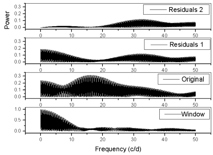
Fig. 2 The analysis of Period04 is presented. At the bottom is the window function. Going upwards, the second panel shows the periodogram of the original data. The next, the first set of residuals and finally, at the top, the residuals of the second set of residuals.
The other data set analyzed with Period04 was that of the CCD data from TNT observatory. It was homogeneously reduced to the same reference stars. As we can see in Table 1, the first observation of the star was done in March, 2015 and the last in January, 2017, separated by 685 days. The whole sample of CCD data is constituted of ten nights. The analysis gave the results listed in Table 4 with a zero point of −0.0102. If we consider 50.412021 (= 3F1) the residuals diminish to 0.03736.
3.3. O-C Differences
Before calculating the coefficients of the ephemeris equation, we studied the existing literature related to KZ Hya. Several authors have conducted studies of the O-C behavior of these particular objects, and in this preliminary stage we took the existing equations and reproduced the diagrams with our updated list of times of maxima taken from literature plus the data that we observed. These reported ephemerides are listed in Table 2 and shown schematically in Figure 7 in which the newly observed ephemerides are also presented.
Table 2 contains a compilation of the equation ephemerides reported in the literature, namely, those of Doncel et al. (2005), Chulee Kim et al. (2007) and Fu et al. (2008) as well as the results of the analysis of the present paper. The goodness of each was evaluated by calculating the O-C mean standard deviation value which is presented in the fifth column of Table 2 utilizing all the available times of maximum data, a more extended set than that the pioneer researchers had in the past. Columns two, three and four list the equation ephemerides elements. Finally, the goodness of each proposed period was evaluated in Period04 through the reported residuals provided in the code. These are listed in last column of Table 2.
Since the study of Fu et al. (2008) (with a time basis of 11670 days, almost 32 years), more observations have been realized, some of them carried out recently, and they are presented in this paper in Table 1 (the time basis has been extended to 14955 days or nearly 9 years more, almost one third more than what Fu et al. (2008) used for their calculations). We tested the old proposed ephemerides equations with the complete set of times of maximum light which includes 221 times of maximum light.
3.4. Period Determination through O-C Differences Minimization (PDDM)
We also employed a method based on the idea of searching the minimization of the chord length linking all the points in the O-C diagram for different values of changing periods, looking for the best period which corresponds to the minimum chord length (See the case of BO Lyn, Peña et al. 2016).
A set of 221 times of maxima was considered to perform this analysis. Taking this into consideration, we determined an interval span in which the period is located at 0.0594±0.0003 days. Maintaining a period precision of a billionth and taking the interval span period into consideration, 626541 periods were used to perform this method. The T0 used to calculate the O-C diagrams is 2457772.8602. Then the best period is the one with the smallest chord length and it is shown in Figure 3. The resulting linear ephemerides equation is

Figure 4 shows the respective O-C diagram of the period found. As a part of the analysis, we also performed a search for a possible sinusoidal behavior in the O-C diagram. This kind of behavior is related to the light-travel time effect (LTTE) due to the presence of a second body orbiting the main body.
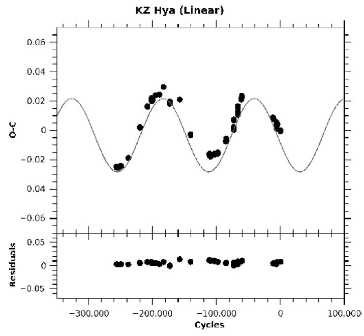
Fig. 4 Period determination through an O-C differences minimization with a sinusoidal fit assuming a linear behavior in the ephemerides equation and the resiudals, PDDM.
As can be seen in Figure 4, the diagram appears to have a clear sinusoidal behavior. Then, we adjusted a sinusoidal function to the O-C diagram performing a fit using the Levenberg-Marquardt algorithm. The fitting equation for the O-C diagram is
where Z is the Y interception; A is the amplitude in days; ω, the frequency in 1/E, and φ, the phase. The continuous line in Figure 4 shows the sinusoidal fit over the O-C diagram.
The sinusoidal function parameters are listed in Table 6. According to this, the period of the sinusoidal behavior is 8495.42 days or 23.28 years.
Looking at the O-C diagram and the sinusoidal adjustment of Figure 4, it is possible to see an ascending branch in the O-C diagram, a behavior that can be caused by a secular variation in the intrinsic period of the pulsating star, i.e., KZ Hya. Following the same PDDM method, a sinusoidal adjustment was performed this time including a quadratic term and a correction term for the period. These components are the β in the quadratic ephemerides equation of this system and a dP. The fit is shown in Figure 5 and the sinusoidal function parameters are listed in Table 6. According to this new model, the period of the second body that is observed by the LTTE is 8659.83 days or 23.73 years and the resulting ephemerides equation is
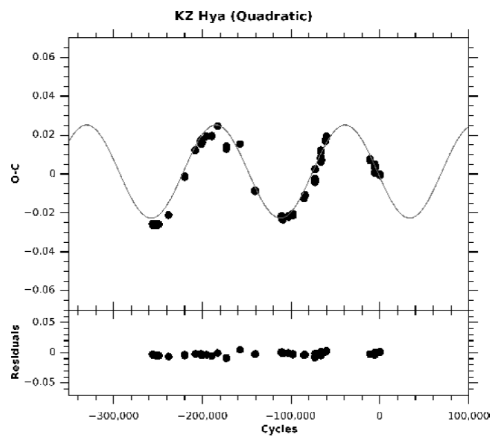
Fig. 5 Period determination through an O-C differences minimization with a sinusoidal fit over a quadratic behavior in the ephemerides equation and the residuals, PDDM.
The goodness of the model is determined by the RSS residuals listed in Table 5 and Table 6 showing that the model with the secular variation (quadratic) is the one that fits the O-C behavior better.
Table 5 Equation parameters for the sinusoidal fit of the O-C residuals.*
| Value | Error | |
|---|---|---|
| Z | −3.338 × 10⁻³ | 2.416 × 10⁻⁴ |
| Ω | 7.005 × 10⁻⁶ | 2.431 × 10⁻⁸ |
| A | 2.505 × 10⁻² | 3.116 × 10⁻⁴ |
| Φ | 5.354 × 10⁻¹ | 2.614 × 10⁻³ |
| RSS residuals | 2.695 × 10⁻³ |
*For the linear fit.
Table 6 Equation parameters for the sinusoidal fit of the O-C residuals.*
| Value | Error | |
|---|---|---|
| Z | 3.629 × 10⁻³ | 2.554 × 10⁻⁴ |
| Ω | 6.921 × 10⁻⁶ | 2.641 × 10⁻⁸ |
| A | 2.429 × 10⁻² | 2.821 × 10⁻⁴ |
| Φ | 5.288 × 10⁻¹ | 2.487 × 10⁻³ |
| β | 6.473 × 10⁻¹³ | 7.983 × 10⁻¹⁴ |
| dP | 7.056 × 10⁻⁸ | 1.06 × 10⁻⁸ |
| RSS residuals | 2.370 × 10⁻³ |
*For the quadratic adjustment.
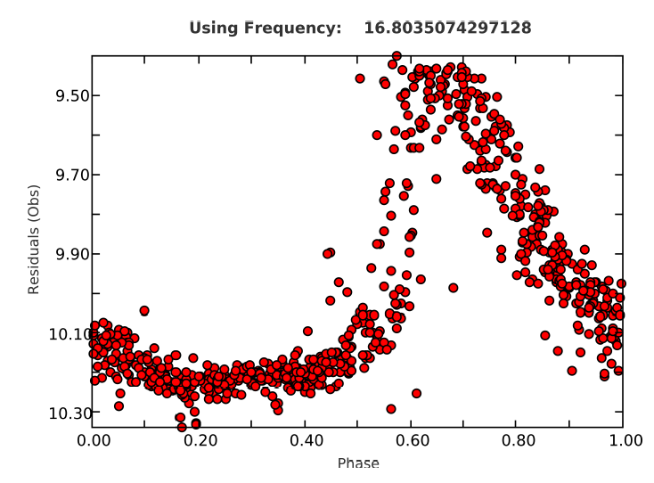
3.5. Phase Dispersion Minimization of Kepler’s Data
Another independent source of data was considered: the Kepler field. This is a set with little data on KZ Hya although it has been densely observed. In their package http://www.astrouw.edu.pl/asas/?page=aasc, a visualization of both the data set and a window to test different periods directly is provided. Starting from scratch, we took as seed the root of all previously determined periods up to four decimal figures. Looking at the phase diagrams we were refining, the periods were modified considering the phase dispersion as criterion of goodness. Finally, a value of 0.059511385 d gave the best phase diagram (Figure 6). The result is included in Table 2 along with the other methods and data sets.
3.6. Period Determination Conclusions
Up to now, KZ Hya had been observed extensively and analyzed carefully. In the past there were extensive studies which have been previously mentioned (see Boonyarak et al. (2011) and bibliography therein).
Since then, more information was gathered but no period analysis was done. In the present paper, different approaches were utilized to determine the stability of the pulsation.
In the first approach, differences of consecutive times of maximum light were evaluated to determine a coarse period; the second method utilized time series analyses of two different data sets. The first set is that of the V filter of the photometry of McNamara & Brudge (1985) and that of the uvby − β photoelectric of the present paper. In this case the time span covered is 13798.3358 d or 38 years, which in cycles is 231864. The amazing result is that the uvby − β photoelectric photometry both in magnitude and color indexes fit remarkably well the phase diagram despite the large time gap in between. The other set is that of the present paper’s CCD photometry.
With respect to the third method, utilizing the set of 222 times of maximum light, including those recently observed (15256 days or 256372 cycles apart), there are three studies in the literature, Chulee et al. (2007), Fu et al. (2008) and Boonyarak et al. (2011), whose residuals show a very distinct sinusoid behavior or residuals that could be interpreted as a LTTE of a binary nature. This result is derived with the PDDM method constructed in the present paper.
The remaining methods like those of Doncel et al. (2005) and those of Period04 show residuals without such a pattern. The fourth method utilized the data collected by Kepler for which we adjusted the period by an eye-ball phase dispersion minimization. The summary of the behavior of all the proposed period calculations (O-C) vs Epoch is presented in Table 2.
Basing our analysis of the most simple results we must consider the overall behavior presented in Table 2 and Figure 7. To begin with, we preferred those ephemerides equations with O-C sinusoidal residuals because they are supported by physical arguments. With this idea in mind, we discarded the period proposed from the O-C differences of the consecutive times of maxima (0.059399998 d) because this analysis only pursued the corroboration of the already published results. Given the relatively few pairs of data, the resulting accuracy is not sufficient, but served its purpose to coarsely verify the correctness of the values of the proposed periods in the literature. Now, analyzing the different O-C residuals of the different ephemerides equations proposed, we have to discard those of Doncel et al. (2005), because it seems that the times of maximum light they published are incorrect, and hence cause an erroneous ephemerides equation. In fact, Fu et al. (2008) states that “the observations of Doncel et al. (2005) covered 12 maximum phases of KZ Hya. However, this work had a significant error in the computation of Julian Dates which took UT = 0h as the reference time of the Julian Date calculation, instead of UT=12h”. Two more proposed ephemerides should not be taken into consideration: the two obtained by the time series analysis by Fourier transforms in Period04. It is encouraging that with such a long time of separation between the considered two uvby data sets: McNamara & Brudge (1985) and the present paper’s data, this analysis gave an amazing phase diagram. However, the period (0.060742815 d), corresponding to the best frequency in Period04, differs significantly from the O-C results of the times of maxima and is not even close to the period obtained by the O-C differences.

Table 7 Transformation coefficients obtained for the observed season
| Season | B | D | F | J | H | I | L |
|---|---|---|---|---|---|---|---|
| Jan 2016 | 0.031 | 1.008 | 1.031 | -0.004 | 1.015 | 0.159 | -1.362 |
| σ | 0.028 | 0.003 | 0.015 | 0.017 | 0.005 | 0.004 | 0.060 |
Such a large discrepancy is not found when the CCD data is analyzed by Period04. This set, however, has the disadvantage of having a very short time span and hence the result cannot be as accurate as that obtained from the O-C analysis that utilizes all the times of maximum light in a larger time span. The same conclusion can be drawn from Kepler’s data and methodology.
In conclusion, there are three analyses with congruent results: Chulee et al. (2007), Fu et al. (2008) and PDDM (present paper). The three methods analyzed the extended data sets up to the current date and gave the same behavior of the residuals. They are also numerically very close: 0.059510388 d for Chulee et al. (2007); 0.059510413 for Fu et al. (2008) and 0.059510396 d for PDDM. Their average value gives 0.059510399 ± 1.3 × 10⁻⁸ and the corresponding differences with mean value of −1.1×10⁻⁸, 1.4 × 10⁻⁸ and −3 × 10⁻⁹, almost negligible but not equal. We feel that with a longer time basis this puzzle will be solved.
4. Physical parameters
4.1. Data Acquisition and Reduction at SPM
The observations were done in January, 2016 along with some other variable stars and clusters. The procedure to determine the physical parameters has been reported elsewhere (Peña et al., 2016). If the photometric system is well-defined and calibrated, it provides an efficient way to investigate physical conditions such as effective temperature and surface gravity via a direct comparison of the unreddened indexes with the theoretical models. These calibrations have already been described and used in previous analyses, (Peña & Peniche; 1994; Peña & Sareyan, 2006).
A comparison of theoretical models, such as those of Lester, Gray & Kurucz (1986), (hereinafter LGK86) with intermediate or wide band photometry measured for each star, allows the determination of reddening. LGK86 calculated grids for stellar atmospheres for G, F, A, B and O stars for different values of [Fe/H] in a temperature range from 5500 up to 50 000 K. The surface gravities vary approximately from the Main Sequence values to the limit of the radiation pressure in 0.5 intervals in log g. A comparison between the photometric unreddened indexes (b − y)0 and c0 obtained for the star with the models allows us to determine the effective temperature Te and surface gravity log g.
These calibrations might be either those proposed by Balona & Shobbrook (1984) and Shobbrook (1984) for early type stars, or those proposed by Nissen (1988) for A and F type stars. Therefore, it is necessary to first determine the range of variation in spectral class of KZ Hya. This will be accomplished by means of the unreddened [m1], [c1] and [u-b] color indexes.
According to Simbad, KZ Hya has a spectral type of B9 III/IV, and therefore, the first method should be adequate. However, if the uvby − β photoelectric photometry obtained in the present work is utilized to determine the spectral type, for example in the [m1 ] vs. [c1 ] diagram of Golay (1974), Figure 8, it is immediately seen that KZ Hya is not such an early A type star as was reported, but a later type, and hence Nissen’s (1988) procedure is applicable.
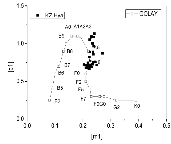
Table 8 uvby − β photoelectric photometry of KZ Hya
| HJD | V | (b − y) | m1 | c1 | β | [m1] | [c1] | [u − b] |
|---|---|---|---|---|---|---|---|---|
| -2457000 | ||||||||
| 399.8477 | 11.875 | 0.130 | 0.195 | 0.928 | 2.706 | 0.237 | 0.902 | 1.375 |
| 399.8506 | 11.865 | 0.160 | 0.154 | 0.952 | 2.754 | 0.205 | 0.920 | 1.330 |
| 399.8546 | 11.897 | 0.149 | 0.186 | 0.872 | 2.743 | 0.234 | 0.842 | 1.310 |
| 399.8567 | 11.894 | 0.162 | 0.180 | 0.865 | 2.791 | 0.232 | 0.833 | 1.296 |
| 399.8591 | 11.901 | 0.172 | 0.169 | 0.881 | 2.774 | 0.224 | 0.847 | 1.295 |
| 399.8617 | 11.937 | 0.160 | 0.167 | 0.893 | 2.804 | 0.218 | 0.861 | 1.297 |
| 399.8638 | 11.944 | 0.166 | 0.177 | 0.881 | 2.751 | 0.230 | 0.848 | 1.308 |
| 399.8662 | 11.974 | 0.164 | 0.157 | 0.882 | 2.683 | 0.209 | 0.849 | 1.268 |
| 399.8706 | 11.980 | 0.193 | 0.139 | 0.877 | 2.730 | 0.201 | 0.838 | 1.240 |
| 399.8728 | 11.974 | 0.210 | 0.123 | 0.877 | 2.695 | 0.190 | 0.835 | 1.215 |
| 399.8747 | 11.999 | 0.195 | 0.157 | 0.833 | 2.682 | 0.219 | 0.794 | 1.233 |
| 399.8768 | 12.012 | 0.192 | 0.167 | 0.824 | 2.664 | 0.228 | 0.786 | 1.242 |
| 399.8790 | 12.015 | 0.206 | 0.135 | 0.856 | 2.731 | 0.201 | 0.815 | 1.217 |
| 399.8809 | 12.056 | 0.155 | 0.222 | 0.802 | 2.691 | 0.272 | 0.771 | 1.314 |
| 399.8846 | 12.076 | 0.157 | 0.215 | 0.784 | 2.675 | 0.265 | 0.753 | 1.283 |
| 399.8864 | 12.064 | 0.174 | 0.190 | 0.812 | 2.713 | 0.246 | 0.777 | 1.269 |
| 399.8895 | 12.057 | 0.188 | 0.178 | 0.791 | 2.698 | 0.238 | 0.753 | 1.230 |
| 399.8926 | 12.059 | 0.196 | 0.155 | 0.830 | 2.694 | 0.218 | 0.791 | 1.226 |
| 399.8946 | 12.061 | 0.181 | 0.171 | 0.823 | 2.715 | 0.229 | 0.787 | 1.245 |
| 399.8966 | 11.964 | 0.253 | 0.121 | 0.717 | 2.739 | 0.202 | 0.666 | 1.070 |
| 399.9008 | 11.956 | 0.247 | 0.118 | 0.739 | 2.730 | 0.197 | 0.690 | 1.084 |
| 399.9027 | 11.962 | 0.232 | 0.115 | 0.791 | 2.708 | 0.189 | 0.745 | 1.123 |
| 399.9049 | 11.950 | 0.224 | 0.139 | 0.751 | 2.719 | 0.211 | 0.706 | 1.128 |
| 399.9073 | 11.939 | 0.205 | 0.148 | 0.795 | 2.715 | 0.214 | 0.754 | 1.181 |
| 399.9093 | 11.907 | 0.221 | 0.124 | 0.792 | 2.717 | 0.195 | 0.748 | 1.137 |
| 399.9114 | 11.955 | 0.173 | 0.162 | 0.869 | 2.777 | 0.217 | 0.834 | 1.269 |
| 399.9157 | 11.916 | 0.167 | 0.159 | 0.878 | 2.731 | 0.212 | 0.845 | 1.269 |
| 399.9176 | 11.918 | 0.161 | 0.173 | 0.907 | 2.811 | 0.225 | 0.875 | 1.324 |
| 399.9193 | 11.878 | 0.168 | 0.151 | 0.913 | 2.792 | 0.205 | 0.879 | 1.289 |
| 399.9208 | 11.911 | 0.135 | 0.190 | 0.912 | 2.743 | 0.233 | 0.885 | 1.351 |
| 399.9224 | 11.857 | 0.163 | 0.163 | 0.891 | 2.757 | 0.215 | 0.858 | 1.289 |
| 399.9240 | 11.840 | 0.153 | 0.160 | 0.950 | 2.742 | 0.209 | 0.919 | 1.337 |
| 399.9257 | 11.828 | 0.151 | 0.163 | 0.925 | 2.777 | 0.211 | 0.895 | 1.317 |
| 399.9276 | 11.833 | 0.142 | 0.176 | 0.911 | 2.770 | 0.221 | 0.883 | 1.325 |
| 401.9013 | 11.842 | 0.155 | 0.171 | 0.918 | 2.764 | 0.221 | 0.887 | 1.328 |
| 401.9033 | 11.838 | 0.159 | 0.164 | 0.923 | 2.796 | 0.215 | 0.891 | 1.321 |
| 401.9052 | 11.845 | 0.180 | 0.146 | 0.939 | 2.799 | 0.204 | 0.903 | 1.310 |
| 401.9070 | 11.863 | 0.167 | 0.166 | 0.901 | 2.773 | 0.219 | 0.868 | 1.306 |
| 401.9086 | 11.879 | 0.157 | 0.177 | 0.913 | 2.789 | 0.227 | 0.882 | 1.336 |
| 401.9103 | 11.888 | 0.169 | 0.151 | 0.934 | 2.779 | 0.205 | 0.900 | 1.310 |
| 401.9135 | 11.909 | 0.152 | 0.195 | 0.878 | 2.730 | 0.244 | 0.848 | 1.335 |
| 401.9152 | 11.897 | 0.171 | 0.173 | 0.895 | 2.794 | 0.228 | 0.861 | 1.316 |
| 401.9168 | 11.914 | 0.187 | 0.144 | 0.909 | 2.774 | 0.204 | 0.872 | 1.279 |
| 401.9187 | 11.927 | 0.173 | 0.173 | 0.895 | 2.794 | 0.228 | 0.860 | 1.317 |
| 401.9207 | 11.921 | 0.189 | 0.164 | 0.866 | 2.783 | 0.224 | 0.828 | 1.277 |
| 401.9227 | 11.951 | 0.182 | 0.164 | 0.875 | 2.788 | 0.222 | 0.839 | 1.283 |
| 401.9245 | 11.964 | 0.185 | 0.153 | 0.893 | 2.806 | 0.212 | 0.856 | 1.280 |
| 401.9264 | 11.961 | 0.202 | 0.133 | 0.881 | 2.766 | 0.198 | 0.841 | 1.236 |
| 401.9301 | 11.969 | 0.195 | 0.174 | 0.855 | 2.746 | 0.236 | 0.816 | 1.289 |
| 401.9319 | 11.983 | 0.187 | 0.184 | 0.825 | 2.753 | 0.244 | 0.788 | 1.275 |
| 401.9337 | 11.992 | 0.199 | 0.169 | 0.829 | 2.802 | 0.233 | 0.789 | 1.255 |
| 401.9362 | 12.000 | 0.204 | 0.162 | 0.814 | 2.719 | 0.227 | 0.773 | 1.228 |
| 401.9378 | 12.005 | 0.217 | 0.146 | 0.822 | 2.753 | 0.215 | 0.779 | 1.209 |
| 401.9395 | 12.015 | 0.208 | 0.155 | 0.834 | 2.743 | 0.222 | 0.792 | 1.236 |
| 401.9411 | 12.039 | 0.195 | 0.159 | 0.827 | 2.728 | 0.221 | 0.788 | 1.231 |
| 401.9430 | 12.033 | 0.218 | 0.147 | 0.790 | 2.769 | 0.217 | 0.746 | 1.180 |
| 401.9450 | 12.030 | 0.231 | 0.121 | 0.825 | 2.769 | 0.195 | 0.779 | 1.169 |
| 401.9469 | 12.039 | 0.212 | 0.133 | 0.852 | 2.734 | 0.201 | 0.810 | 1.211 |
| 401.9509 | 12.033 | 0.231 | 0.130 | 0.837 | 2.672 | 0.204 | 0.791 | 1.199 |
| 401.9526 | 12.046 | 0.219 | 0.141 | 0.812 | 2.670 | 0.211 | 0.768 | 1.190 |
| 401.9547 | 12.058 | 0.193 | 0.159 | 0.829 | 2.784 | 0.221 | 0.790 | 1.232 |
| 401.9567 | 12.031 | 0.210 | 0.146 | 0.811 | 2.770 | 0.213 | 0.769 | 1.195 |
| 401.9586 | 12.025 | 0.203 | 0.151 | 0.830 | 2.773 | 0.216 | 0.789 | 1.221 |
| 401.9610 | 12.010 | 0.212 | 0.147 | 0.810 | 2.758 | 0.215 | 0.768 | 1.197 |
| 401.9631 | 12.015 | 0.183 | 0.185 | 0.791 | 2.770 | 0.244 | 0.754 | 1.242 |
| 401.9652 | 11.990 | 0.187 | 0.176 | 0.818 | 2.791 | 0.236 | 0.781 | 1.252 |
| 401.9677 | 11.959 | 0.213 | 0.137 | 0.845 | 2.779 | 0.205 | 0.802 | 1.213 |
| 401.9697 | 11.971 | 0.170 | 0.169 | 0.836 | 2.753 | 0.223 | 0.802 | 1.249 |
| 401.9714 | 11.921 | 0.190 | 0.156 | 0.863 | 2.747 | 0.217 | 0.825 | 1.259 |
| 401.9735 | 11.913 | 0.188 | 0.147 | 0.868 | 2.828 | 0.207 | 0.830 | 1.245 |
| 401.9772 | 11.891 | 0.185 | 0.148 | 0.885 | 2.779 | 0.207 | 0.848 | 1.262 |
| 401.9791 | 11.885 | 0.166 | 0.176 | 0.866 | 2.751 | 0.229 | 0.833 | 1.291 |
| 401.9812 | 11.846 | 0.166 | 0.154 | 0.920 | 2.781 | 0.207 | 0.887 | 1.301 |
| 401.9832 | 11.828 | 0.171 | 0.150 | 0.919 | 2.817 | 0.205 | 0.885 | 1.294 |
| 401.9852 | 11.814 | 0.179 | 0.132 | 0.948 | 2.810 | 0.189 | 0.912 | 1.291 |
| 401.9869 | 11.813 | 0.166 | 0.144 | 0.940 | 2.833 | 0.197 | 0.907 | 1.301 |
The application of the above mentioned numerical unreddening package gives the results listed in Table 9 for KZ Hya. This table lists, ordered in decreasing Hβ, in the first column, the HJD; subsequent columns present the reddening, the unreddened indexes, the unreddened and the absolute magnitudes. Mean values were calculated for E(b − y) for two cases: (i) the whole data sample and (ii) in phase limits between 0.3 and 0.8, which is customary for pulsating stars to avoid the maximum. This gave values for the whole cycle of 0.075 ± 0.027; 9.04 ± 0.80 and 687 ± 256 for E(b − y), DM and distance (in pc), respectively, whereas for the mentioned phase limits we obtained, 0.073 ± 0.030; 9.02 ± 0.93 and 696 ± 297 respectively. The uncertainty is merely the standard deviation. In the case of the reddening, most of the values in the spectral type in the F stage of KZ Hya produced negative values which is un-physical. In those cases we forced the reddening to be zero. If the negative values are included, the mean E(b − y) is 0.009 ± 0.038.
Table 9 Reddening and unreddened parameters of KZ Hya
| HJD | E(b − y) | (b − y)0 | m0 | c0 | Hβ | V0 | MV |
|---|---|---|---|---|---|---|---|
| -2457000.00 | |||||||
| 401.9869 | .063 | .166 | .163 | .927 | 2.833 | 11.54 | 1.76 |
| 401.9735 | .074 | .188 | .169 | .853 | 2.828 | 11.60 | 2.35 |
| 401.9832 | .052 | .171 | .166 | .909 | 2.817 | 11.60 | 1.76 |
| 399.9176 | .036 | .161 | .184 | .900 | 2.811 | 11.76 | 1.78 |
| 401.9852 | .058 | .179 | .149 | .936 | 2.810 | 11.57 | 1.40 |
| 401.9245 | .055 | .185 | .170 | .882 | 2.806 | 11.73 | 1.83 |
| 399.8617 | .028 | .160 | .176 | .887 | 2.804 | 11.81 | 1.80 |
| 401.9337 | .059 | .199 | .187 | .817 | 2.802 | 11.74 | 2.35 |
| 401.9052 | .049 | .180 | .161 | .929 | 2.799 | 11.63 | 1.31 |
| 401.9033 | .024 | .159 | .171 | .918 | 2.796 | 11.73 | 1.41 |
| 401.9152 | .032 | .171 | .183 | .889 | 2.794 | 11.76 | 1.63 |
| 401.9187 | .034 | .173 | .183 | .888 | 2.794 | 11.78 | 1.63 |
| 399.9193 | .029 | .168 | .160 | .907 | 2.792 | 11.75 | 1.44 |
| 399.8567 | .017 | .162 | .185 | .862 | 2.791 | 11.82 | 1.86 |
| 401.9652 | .038 | .187 | .187 | .810 | 2.791 | 11.83 | 2.28 |
| 401.9086 | .015 | .157 | .182 | .910 | 2.789 | 11.81 | 1.40 |
| 401.9227 | .036 | .182 | .175 | .868 | 2.788 | 11.80 | 1.73 |
| 401.9547 | .039 | .193 | .171 | .821 | 2.784 | 11.89 | 2.08 |
| 401.9207 | .038 | .189 | .175 | .858 | 2.783 | 11.76 | 1.73 |
| 401.9812 | .019 | .166 | .160 | .916 | 2.781 | 11.77 | 1.21 |
| 401.9103 | .022 | .169 | .157 | .930 | 2.779 | 11.80 | 1.06 |
| 401.9677 | .057 | .213 | .154 | .834 | 2.779 | 11.72 | 1.86 |
| 401.9772 | .033 | .185 | .158 | .878 | 2.779 | 11.75 | 1.50 |
| 399.9114 | .017 | .173 | .167 | .866 | 2.777 | 11.88 | 1.61 |
| 399.9257 | .001 | .151 | .163 | .925 | 2.777 | 11.82 | 1.11 |
| 399.8591 | .015 | .172 | .174 | .878 | 2.774 | 11.84 | 1.46 |
| 401.9168 | .033 | .187 | .154 | .902 | 2.774 | 11.77 | 1.21 |
| 401.9070 | .011 | .167 | .169 | .899 | 2.773 | 11.81 | 1.27 |
| 401.9586 | .040 | .203 | .163 | .822 | 2.773 | 11.85 | 1.91 |
| 399.9276 | .000 | .142 | .176 | .911 | 2.770 | 11.83 | 1.13 |
| 401.9567 | .043 | .210 | .159 | .802 | 2.770 | 11.85 | 2.03 |
| 401.9631 | .014 | .183 | .189 | .788 | 2.770 | 11.95 | 2.21 |
| 401.9430 | .048 | .218 | .161 | .780 | 2.769 | 11.83 | 2.21 |
| 401.9450 | .065 | .231 | .140 | .812 | 2.769 | 11.75 | 1.89 |
| 401.9264 | .039 | .202 | .145 | .873 | 2.766 | 11.79 | 1.34 |
| 401.9013 | .000 | .155 | .171 | .918 | 2.764 | 11.84 | 0.98 |
| 401.9610 | .035 | .212 | .158 | .803 | 2.758 | 11.86 | 1.86 |
| 399.9224 | .000 | .163 | .163 | .891 | 2.757 | 11.86 | 1.12 |
| 399.8506 | .000 | .160 | .154 | .952 | 2.754 | 11.86 | 0.53 |
| 401.9319 | .008 | .187 | .186 | .823 | 2.753 | 11.95 | 1.66 |
| 401.9378 | .038 | .217 | .157 | .814 | 2.753 | 11.84 | 1.68 |
| 401.9697 | .000 | .170 | .169 | .836 | 2.753 | 11.97 | 1.56 |
| 399.8638 | .000 | .166 | .177 | .881 | 2.751 | 11.94 | 1.12 |
| 401.9791 | .000 | .166 | .176 | .866 | 2.751 | 11.89 | 1.26 |
| 401.9714 | .010 | .190 | .159 | .861 | 2.747 | 11.88 | 1.23 |
| 401.9301 | .013 | .195 | .178 | .852 | 2.746 | 11.91 | 1.29 |
| 399.8546 | .000 | .149 | .186 | .872 | 2.743 | 11.90 | 1.09 |
| 399.9208 | .000 | .135 | .190 | .912 | 2.743 | 11.91 | 0.73 |
| 401.9395 | .022 | .208 | .162 | .830 | 2.743 | 11.92 | 1.44 |
| 399.9240 | .000 | .153 | .160 | .950 | 2.742 | 11.84 | 0.38 |
| 399.8966 | .052 | .253 | .137 | .707 | 2.739 | 11.74 | 2.42 |
| 401.9469 | .021 | .212 | .139 | .848 | 2.734 | 11.95 | 1.09 |
| 399.8790 | .014 | .206 | .139 | .853 | 2.731 | 11.96 | 0.98 |
| 399.9157 | .000 | .167 | .159 | .878 | 2.731 | 11.92 | 0.79 |
| 399.8706 | .002 | .193 | .140 | .877 | 2.730 | 11.97 | 0.77 |
| 399.9008 | .042 | .247 | .131 | .731 | 2.730 | 11.77 | 2.01 |
| 401.9135 | .000 | .152 | .195 | .878 | 2.730 | 11.91 | 0.76 |
| 401.9411 | .000 | .195 | .159 | .827 | 2.728 | 12.04 | 1.17 |
| 399.9049 | .016 | .224 | .144 | .748 | 2.719 | 11.88 | 1.64 |
| 401.9362 | .000 | .204 | .162 | .814 | 2.719 | 12.00 | 1.07 |
| 399.9093 | .015 | .221 | .129 | .789 | 2.717 | 11.84 | 1.22 |
| 399.8946 | .000 | .181 | .171 | .823 | 2.715 | 12.06 | 0.87 |
| 399.9073 | .000 | .205 | .148 | .795 | 2.715 | 11.94 | 1.13 |
| 399.8864 | .000 | .174 | .190 | .812 | 2.713 | 12.06 | 0.91 |
| 399.9027 | .020 | .232 | .121 | .787 | 2.708 | 11.88 | 0.95 |
| 399.8477 | .000 | .130 | .195 | .928 | 2.706 | 11.88 | −0.44 |
| 399.8895 | .000 | .188 | .178 | .791 | 2.698 | 12.06 | 0.60 |
| 399.8728 | .000 | .210 | .123 | .877 | 2.695 | 11.97 | −0.40 |
| 399.8926 | .000 | .196 | .155 | .830 | 2.694 | 12.06 | 0.04 |
| 399.8809 | .000 | .155 | .222 | .802 | 2.691 | 12.06 | 0.20 |
| 399.8662 | .000 | .164 | .157 | .882 | 2.683 | 11.97 | −0.98 |
| 399.8747 | .000 | .195 | .157 | .833 | 2.682 | 12.00 | −0.49 |
| 399.8846 | .000 | .157 | .215 | .784 | 2.675 | 12.08 | −0.19 |
| 401.9509 | .000 | .231 | .130 | .837 | 2.672 | 12.03 | −0.89 |
| 401.9526 | .000 | .219 | .141 | .812 | 2.670 | 12.05 | −0.68 |
| 399.8768 | .000 | .192 | .167 | .824 | 2.664 | 12.01 | −1.02 |
The same analysis for determining the physical parameters was performed by Fu et al. (2008) by means of uvby − β photoelectric photometry, utilizing Crawford’s (1979) calibrations. They derived an E(b−y) of 0.04±0.01, Te(k) of 7300±530 K, and log g (dex) of 4.00 ± 0.18.
In order to locate our unreddened points in the theoretical grids of LGK86 a metallicity has to be assumed. LGK86 calculated outputs for several metallicities. The metallicity of KZ Hya can be determined from the uvby − β photometry when the star passes through the F type stage (Nissen, 1988). Particularly, in the case of KZ Hya for which we determined a mean metallicity of [Fe/H] = −0.275 ± 0.106 there are two models which were applicable, either [Fe/H] = 0.0 or −0.5. We tested both since our determined mean metallicity lies in-between.
To diminish the noise and to see the variation of the star in phase, mean values of the unreddened colors were calculated in phase bins of 0.1 starting at 0.05 as the initial value. As can be seen in Figure 9, for the case of [Fe/H] = −0.5 the star varies between effective temperature 6800 K and 8100 K; the surface gravity log g varies between 3.2 and 4.0. Table 9 lists these values. Column 1 shows the phase, Columns 2 and 3 list the temperature obtained from the plot for each [Fe/H] value; Column 4, the mean value and Column 5, the standard deviation of the [Fe/H] = −0.5 metallicity. Column 6 shows the effective temperature obtained from the theoretical relation reported by Rodriguez (1989) based on a relation of Petersen & Jorgensen (1972, hereinafter P&J72) Te = 6850 + 1250 × (β − 2.684)/0.144 for each value and averaged in the corresponding phase bin. The last column lists the surface gravity log g from the plot.

4.2. Conclusions on the Physical Parameters
New uvby−β photoelectric photometry observations were carried out for the SX Phe star KZ Hya. From the uvby − β photoelectric photometry we determined first its spectral type, which varies between A5V and A8V, differing from previous determinations. From Nissen’s (1988) calibrations the reddening was determined as well as the unreddened indexes. These served to determine the physical characteristics of this star, log Te, in a range from 6800 K to 8100 K and log g from 3.2 to 3.6 using two methods: (1) from the location of the unreddened indexes in the LGK86 grids, and (2) through the theoretical relation (P&J72). They are similar, within the error bars, and give a good idea of the star’s behavior. Furthermore, when mean values are obtained from the two closest metallicity values, the result is closer to the obtained theoretical value.
5. Conclusions
Rodriguez and Breger’s (2001) in their study on δ Scuti stars, stated in § 2.2 that: “...the distribution in apparent magnitude of the δ Scuti variables known to be part of binary or multiple stellar systems. The R00 catalogue lists 86 variables (62 with CCDM identification). This represents only 14% of the total sample of known δ Scuti stars. Only five variables are fainter than V = 10.0. Hence, multiplicity is catalogued for 22 of all the δ Scuti known up 10. 0. This percentage is very low because more than 50% of the stars are expected to be members of multiple systems”. They later stated that “pulsating stars in eclipsing binaries are important for accurate determinations of fundamental stellar parameters and the study of tidal effects on the pulsations... During the last two decades, unusual changes in the light curves have been detected, leading to a number of different interpretations...
Table 10 effective temperature of KZ Hya as a function of phase
| Phase | Te(0.0) | Te(-0.5) | Mean | σTe | P&J72 | log g(-0.5) |
|---|---|---|---|---|---|---|
| 0.05 | 8000 | 6800 | 7400 | 412 | 7251 | 3.2 |
| 0.15 | 7900 | 6800 | 7350 | 319 | 7235 | 3.4 |
| 0.25 | 8000 | 6800 | 7400 | 267 | 7259 | 3.5 |
| 0.35 | 8000 | 6800 | 7400 | 387 | 7234 | 3.5 |
| 0.45 | 8200 | 7400 | 7800 | 264 | 7494 | 3.6 |
| 0.55 | 8400 | 7900 | 8150 | 284 | 7582 | 3.6 |
| 0.65 | 9000 | 8100 | 8550 | 254 | 7781 | 3.6 |
| 0.75 | 8200 | 7300 | 7750 | 396 | 7469 | 3.4 |
| 0.85 | 8400 | 7900 | 8150 | 164 | 7642 | 3.5 |
| 0.95 | 8200 | 7800 | 8000 | 340 | 7569 | 3.6 |
Note: Values in parenthesis specify the [Fe/H].
“Pulsation provides an additional method to detect multiplicity through a study of the light-time effects in a binary system. This method generally favors high-amplitude variables with only one or two pulsation periods (which tend to be radial). Several decades of measurements are usually required to study these (O-C) residuals in the times of maxima”.
At that time they listed, in their Table 4, only six stars with determined orbital periods. Since then, with a longer time basis for those stars, and for an increased number of measured times of maximum, better defined orbital elements have been obtained. There have been numerous studies with this purpose on HADS stars. For example, Boonyarak et al. (2011) carried out a study devoted to the analysis the stability of fourteen HADS stars. Many other authors carried out analyses on a star-by-star basis. Some of the HADS stars show a behavior of the O-C residuals compatible with the light-travel time effect pointing to a binary nature: AD CMi, KZ Hya, AN Lyn, BE Lyn, SZ Lyn, BP Peg, BS Aqr, CY Aqr among others, whereas there are some that, on the contrary, vary with one period and its harmonics and do not show this effect. To this category, according to Boonyarak et al., (2011) belong GP And, AZ CMi, AE UMa, RV Ari, DY Her, DH Peg.
In the present study we found that KZ Hya has a spectral type varying between A5V and A8V, values of E(b-y) of 0.073 ± 0.030, DM of 9.02 ± 0.93. It has been proved that KZ Hya is pulsating with one stable varying period (0.059510382 d), whose O-C residuals show a sinusoidal pattern compatible with a light-travel time effect. As regards this topic, it is interesting to mention that in his excellent discussion, Templeton (2005) states that: “In all cases except SZ Lyn, the period of the purported binarity is close to that of the duration of the (O-C) measurements, making it difficult to prove that the signal is truly sinusoidal. A sinusoidal interpretation is only reliable when multiple cycles are recorded, as in SZ Lyn. While the binary hypothesis is certainly possible in most of these cases, conclusive proof will not be available for years or even decades to come. Continued monitoring of times of maximum will be crucial, and such observations are encouraged. In the meantime, however, other possible interpretations of their behavior must also be explored”.
We feel that the results presented in this paper agree with Templeton’s (2005) request that “a sinusoidal interpretation is only reliable when multiple cycles are recorded” as we have found for KZ Hya.
We would like to thank the staff of the OAN at SPM and Tonantzintla for their assistance in securing the observations. This work was partially supported by the OAD of the IAU (ESAOBEL), PAPIIT IN104917 and PAPIME PE113016. Proofreading and typing were done by J. Miller and J. Orta, respectively. C. Guzmán, F. Ruiz and A. Díaz assisted us in the computing and we thank B. Juárez and G. Pérez for bibliographic help. All the students thank the IA for allotting telescope time. Special thanks to H. Huepa and A. Pani for the observations and discussions. We acknowledge the comments and suggestions of an anonymous referee that improved this paper. We have made use of the SIMBAD databases operated at CDS, Strasbourg, France; NASA ADS Astronomy Query Form.

